Introduction
The notebook extends the console-based approach to interactive computing in
a qualitatively new direction, providing a web-based application suitable for
capturing the whole computation process: developing, documenting, and
executing code, as well as communicating the results. The Jupyter notebook
combines two components:
A web application: a browser-based tool for interactive authoring of
documents which combine explanatory text, mathematics, computations and their
rich media output.
Notebook documents: a representation of all content visible in the web
application, including inputs and outputs of the computations, explanatory
text, mathematics, images, and rich media representations of objects.
Main features of the web application
-
In-browser editing for code, with automatic syntax highlighting,
indentation, and tab completion/introspection. -
The ability to execute code from the browser, with the results of
computations attached to the code which generated them. -
Displaying the result of computation using rich media representations, such
as HTML, LaTeX, PNG, SVG, etc. For example, publication-quality figures
rendered by the matplotlib library, can be included inline. -
In-browser editing for rich text using the Markdown markup language, which
can provide commentary for the code, is not limited to plain text. -
The ability to easily include mathematical notation within markdown cells
using LaTeX, and rendered natively by MathJax.
Notebook documents
Notebook documents contains the inputs and outputs of a interactive session as
well as additional text that accompanies the code but is not meant for
execution. In this way, notebook files can serve as a complete computational
record of a session, interleaving executable code with explanatory text,
mathematics, and rich representations of resulting objects. These documents
are internally JSON files and are saved with the .ipynb extension. Since
JSON is a plain text format, they can be version-controlled and shared with
colleagues.
Notebooks may be exported to a range of static formats, including HTML (for
example, for blog posts), reStructuredText, LaTeX, PDF, and slide shows, via
the nbconvert command.
Furthermore, any .ipynb notebook document available from a public
URL can be shared via the Jupyter Notebook Viewer <nbviewer>.
This service loads the notebook document from the URL and renders it as a
static web page. The results may thus be shared with a colleague, or as a
public blog post, without other users needing to install the Jupyter notebook
themselves. In effect, nbviewer is simply nbconvert as
a web service, so you can do your own static conversions with nbconvert,
without relying on nbviewer.
Notebooks and privacy
Because you use Jupyter in a web browser, some people are understandably
concerned about using it with sensitive data.
However, if you followed the standard
install instructions,
Jupyter is actually running on your own computer.
If the URL in the address bar starts with http://localhost: or
http://127.0.0.1:, it’s your computer acting as the server.
Jupyter doesn’t send your data anywhere else—and as it’s open source,
other people can check that we’re being honest about this.
You can also use Jupyter remotely:
your company or university might run the server for you, for instance.
If you want to work with sensitive data in those cases,
talk to your IT or data protection staff about it.
We aim to ensure that other pages in your browser or other users on the same
computer can’t access your notebook server. See Security in the Jupyter notebook server for
more about this.
Starting the notebook server
You can start running a notebook server from the command line using the
following command:
This will print some information about the notebook server in your console,
and open a web browser to the URL of the web application (by default,
http://127.0.0.1:8888).
The landing page of the Jupyter notebook web application, the dashboard,
shows the notebooks currently available in the notebook directory (by default,
the directory from which the notebook server was started).
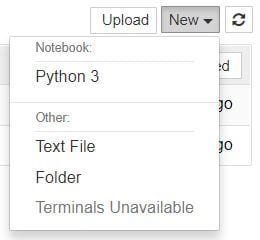
You can create new notebooks from the dashboard with the New Notebook
button, or open existing ones by clicking on their name. You can also drag
and drop .ipynb notebooks and standard .py Python source code files
into the notebook list area.
When starting a notebook server from the command line, you can also open a
particular notebook directly, bypassing the dashboard, with jupyter notebook. The
my_notebook.ipynb.ipynb extension is assumed if no extension is
given.
When you are inside an open notebook, the File | Open… menu option will
open the dashboard in a new browser tab, to allow you to open another notebook
from the notebook directory or to create a new notebook.
Note
You can start more than one notebook server at the same time, if you want
to work on notebooks in different directories. By default the first
notebook server starts on port 8888, and later notebook servers search for
ports near that one. You can also manually specify the port with the
--port option.
Creating a new notebook document
A new notebook may be created at any time, either from the dashboard, or using
the menu option from within an active notebook.
The new notebook is created within the same directory and will open in a new
browser tab. It will also be reflected as a new entry in the notebook list on
the dashboard.

Opening notebooks
An open notebook has exactly one interactive session connected to a
kernel, which will execute code sent by the user
and communicate back results. This kernel remains active if the web browser
window is closed, and reopening the same notebook from the dashboard will
reconnect the web application to the same kernel. In the dashboard, notebooks
with an active kernel have a Shutdown button next to them, whereas
notebooks without an active kernel have a Delete button in its place.
Other clients may connect to the same kernel.
When each kernel is started, the notebook server prints to the terminal a
message like this:
[NotebookApp] Kernel started: 87f7d2c0-13e3-43df-8bb8-1bd37aaf3373
This long string is the kernel’s ID which is sufficient for getting the
information necessary to connect to the kernel. If the notebook uses the IPython
kernel, you can also see this
connection data by running the %connect_info magic, which will print the same ID information along with other
details.
You can then, for example, manually start a Qt console connected to the same
kernel from the command line, by passing a portion of the ID:
$ jupyter qtconsole --existing 87f7d2c0
Without an ID, --existing will connect to the most recently
started kernel.
With the IPython kernel, you can also run the %qtconsole
magic in the notebook to open a Qt console connected
to the same kernel.
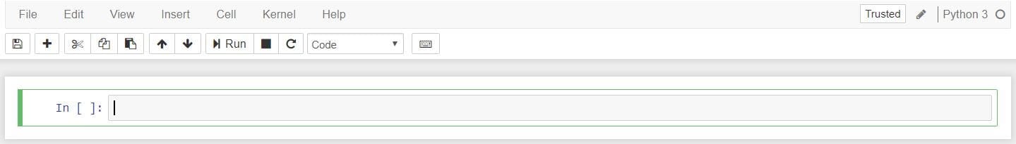
Notebook user interface
When you create a new notebook document, you will be presented with the
notebook name, a menu bar, a toolbar and an empty code cell.

Notebook name: The name displayed at the top of the page,
next to the Jupyter logo, reflects the name of the .ipynb file.
Clicking on the notebook name brings up a dialog which allows you to rename it.
Thus, renaming a notebook
from “Untitled0” to “My first notebook” in the browser, renames the
Untitled0.ipynb file to My first notebook.ipynb.
Menu bar: The menu bar presents different options that may be used to
manipulate the way the notebook functions.
Toolbar: The tool bar gives a quick way of performing the most-used
operations within the notebook, by clicking on an icon.
Code cell: the default type of cell; read on for an explanation of cells.
Structure of a notebook document
The notebook consists of a sequence of cells. A cell is a multiline text input
field, and its contents can be executed by using Shift-Enter, or by
clicking either the “Play” button the toolbar, or Cell, Run in the menu bar.
The execution behavior of a cell is determined by the cell’s type. There are three
types of cells: code cells, markdown cells, and raw cells. Every
cell starts off being a code cell, but its type can be changed by using a
drop-down on the toolbar (which will be “Code”, initially), or via
keyboard shortcuts.
For more information on the different things you can do in a notebook,
see the collection of examples.
Code cells
A code cell allows you to edit and write new code, with full syntax
highlighting and tab completion. The programming language you use depends
on the kernel, and the default kernel (IPython) runs Python code.
When a code cell is executed, code that it contains is sent to the kernel
associated with the notebook. The results that are returned from this
computation are then displayed in the notebook as the cell’s output. The
output is not limited to text, with many other possible forms of output are
also possible, including matplotlib figures and HTML tables (as used, for
example, in the pandas data analysis package). This is known as IPython’s
rich display capability.
Markdown cells
You can document the computational process in a literate way, alternating
descriptive text with code, using rich text. In IPython this is accomplished
by marking up text with the Markdown language. The corresponding cells are
called Markdown cells. The Markdown language provides a simple way to
perform this text markup, that is, to specify which parts of the text should
be emphasized (italics), bold, form lists, etc.
If you want to provide structure for your document, you can use markdown
headings. Markdown headings consist of 1 to 6 hash # signs # followed by a
space and the title of your section. The markdown heading will be converted
to a clickable link for a section of the notebook. It is also used as a hint
when exporting to other document formats, like PDF.
When a Markdown cell is executed, the Markdown code is converted into
the corresponding formatted rich text. Markdown allows arbitrary HTML code for
formatting.
Within Markdown cells, you can also include mathematics in a straightforward
way, using standard LaTeX notation: $...$ for inline mathematics and
$$...$$ for displayed mathematics. When the Markdown cell is executed,
the LaTeX portions are automatically rendered in the HTML output as equations
with high quality typography. This is made possible by MathJax, which
supports a large subset of LaTeX functionality
Standard mathematics environments defined by LaTeX and AMS-LaTeX (the
amsmath package) also work, such as
begin{equation}...end{equation}, and begin{align}...end{align}.
New LaTeX macros may be defined using standard methods,
such as newcommand, by placing them anywhere between math delimiters in
a Markdown cell. These definitions are then available throughout the rest of
the IPython session.
Raw cells
Raw cells provide a place in which you can write output directly.
Raw cells are not evaluated by the notebook.
When passed through nbconvert, raw cells arrive in the
destination format unmodified. For example, you can type full LaTeX
into a raw cell, which will only be rendered by LaTeX after conversion by
nbconvert.
Basic workflow
The normal workflow in a notebook is, then, quite similar to a standard
IPython session, with the difference that you can edit cells in-place multiple
times until you obtain the desired results, rather than having to
rerun separate scripts with the %run magic command.
Typically, you will work on a computational problem in pieces, organizing
related ideas into cells and moving forward once previous parts work
correctly. This is much more convenient for interactive exploration than
breaking up a computation into scripts that must be executed together, as was
previously necessary, especially if parts of them take a long time to run.
To interrupt a calculation which is taking too long, use the Kernel,
Interrupt menu option, or the i,i keyboard shortcut.
Similarly, to restart the whole computational process,
use the Kernel, Restart menu option or 0,0
shortcut.
A notebook may be downloaded as a .ipynb file or converted to a number of
other formats using the menu option File, Download as.
Keyboard shortcuts
All actions in the notebook can be performed with the mouse, but keyboard
shortcuts are also available for the most common ones. The essential shortcuts
to remember are the following:
-
- Shift-Enter: run cell
-
Execute the current cell, show any output, and jump to the next cell below.
If Shift-Enter is invoked on the last cell, it makes a new cell below.
This is equivalent to clicking the Cell, Run menu
item, or the Play button in the toolbar.
-
- Esc: Command mode
-
In command mode, you can navigate around the notebook using keyboard shortcuts.
-
- Enter: Edit mode
-
In edit mode, you can edit text in cells.
For the full list of available shortcuts, click Help,
Keyboard Shortcuts in the notebook menus.
Plotting
One major feature of the Jupyter notebook is the ability to display plots that
are the output of running code cells. The IPython kernel is designed to work
seamlessly with the matplotlib plotting library to provide this functionality.
Specific plotting library integration is a feature of the kernel.
Installing kernels
For information on how to install a Python kernel, refer to the
IPython install page.
The Jupyter wiki has a long list of Kernels for other languages.
They usually come with instructions on how to make the kernel available
in the notebook.
Trusting Notebooks
To prevent untrusted code from executing on users’ behalf when notebooks open,
we store a signature of each trusted notebook.
The notebook server verifies this signature when a notebook is opened.
If no matching signature is found,
Javascript and HTML output will not be displayed
until they are regenerated by re-executing the cells.
Any notebook that you have fully executed yourself will be
considered trusted, and its HTML and Javascript output will be displayed on
load.
If you need to see HTML or Javascript output without re-executing,
and you are sure the notebook is not malicious, you can tell Jupyter to trust it
at the command-line with:
$ jupyter trust mynotebook.ipynb
See Security in notebook documents for more details about the trust mechanism.
Browser Compatibility
The Jupyter Notebook aims to support the latest versions of these browsers:
-
Chrome
-
Safari
-
Firefox
Up to date versions of Opera and Edge may also work, but if they don’t, please
use one of the supported browsers.
Using Safari with HTTPS and an untrusted certificate is known to not work
(websockets will fail).
The Jupyter Notebook is an open-source web application that allows you to create and share documents that contain live code, equations, visualizations, and narrative text. Uses include data cleaning and transformation, numerical simulation, statistical modeling, data visualization, machine learning, and much more. Jupyter has support for over 40 different programming languages and Python is one of them. Python is a requirement (Python 3.3 or greater, or Python 2.7) for installing the Jupyter Notebook itself.
Table Of Content
- Installation
- Starting Jupyter Notebook
- Creating a Notebook
- Hello World in Jupyter Notebook
- Cells in Jupyter Notebook
- Kernel
- Naming the notebook
- Notebook Extensions
Installation
Install Python and Jupyter using the Anaconda Distribution, which includes Python, the Jupyter Notebook, and other commonly used packages for scientific computing and data science. You can download Anaconda’s latest Python3 version from here. Now, install the downloaded version of Anaconda. Installing Jupyter Notebook using pip:
python3 -m pip install --upgrade pip
python3 -m pip install jupyter
Starting Jupyter Notebook
To start the jupyter notebook, type the below command in the terminal.
jupyter notebook
This will print some information about the notebook server in your terminal, including the URL of the web application (by default, http://localhost:8888) and then open your default web browser to this URL.  After the notebook is opened, you’ll see the Notebook Dashboard, which will show a list of the notebooks, files, and subdirectories in the directory where the notebook server was started. Most of the time, you will wish to start a notebook server in the highest level directory containing notebooks. Often this will be your home directory.
Creating a Notebook
To create a new notebook, click on the new button at the top right corner. Click it to open a drop-down list and then if you’ll click on Python3, it will open a new notebook.  The web page should look like this:
Hello World in Jupyter Notebook
After successfully installing and creating a notebook in Jupyter Notebook, let’s see how to write code in it. Jupyter notebook provides a cell for writing code in it. The type of code depends on the type of notebook you created. For example, if you created a Python3 notebook then you can write Python3 code in the cell. Now, let’s add the following code –
Python3
To run a cell either click the run button or press shift ⇧ + enter ⏎ after selecting the cell you want to execute. After writing the above code in the jupyter notebook, the output was:  Note: When a cell has executed the label on the left i.e. ln[] changes to ln[1]. If the cell is still under execution the label remains ln[*].
Cells in Jupyter Notebook
Cells can be considered as the body of the Jupyter. In the above screenshot, the box with the green outline is a cell. There are 3 types of cell:
- Code
- Markup
- Raw NBConverter
Code
This is where the code is typed and when executed the code will display the output below the cell. The type of code depends on the type of the notebook you have created. For example, if the notebook of Python3 is created then the code of Python3 can be added. Consider the below example, where a simple code of the Fibonacci series is created and this code also takes input from the user. Example:  The tex bar in the above code is prompted for taking input from the user. The output of the above code is as follows: Output:
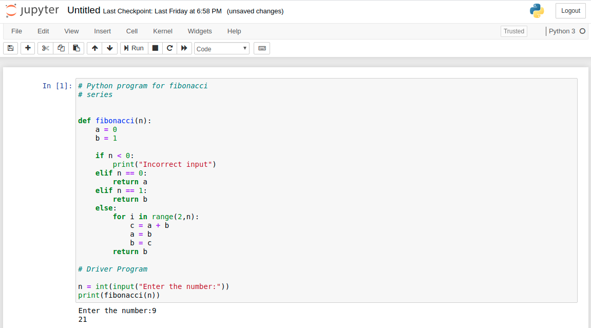
Markdown
Markdown is a popular markup language that is the superset of the HTML. Jupyter Notebook also supports markdown. The cell type can be changed to markdown using the cell menu.  Adding Headers: Heading can be added by prefixing any line by single or multiple ‘#’ followed by space. Example:
  Output:
  Adding List: Adding List is really simple in Jupyter Notebook. The list can be added by using ‘*’ sign. And the Nested list can be created by using indentation. Example:
 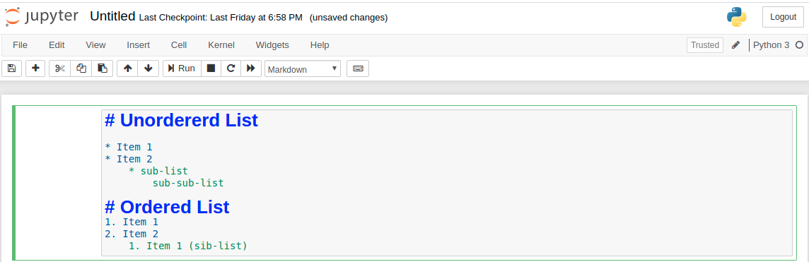 Output:
  Adding Latex Equations: Latex expressions can be added by surrounding the latex code by ‘$’ and for writing the expressions in the middle, surrounds the latex code by ‘$$’. Example:
 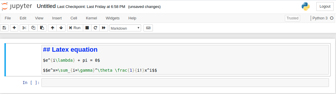 Output:
  Adding Table: A table can be added by writing the content in the following format.
  Output:
  Note: The text can be made bold or italic by enclosing the text in ‘**’ and ‘*’ respectively.
Raw NBConverter
Raw cells are provided to write the output directly. This cell is not evaluated by Jupyter notebook. After passing through nbconvert the raw cells arrives in the destination folder without any modification. For example, one can write full Python into a raw cell that can only be rendered by Python only after conversion by nbconvert.
Kernel
A kernel runs behind every notebook. Whenever a cell is executed, the code inside the cell is executed within the kernel and the output is returned back to the cell to be displayed. The kernel continues to exist to the document as a whole and not for individual cells. For example, if a module is imported in one cell then, that module will be available for the whole document. See the below example for better understanding. Example: 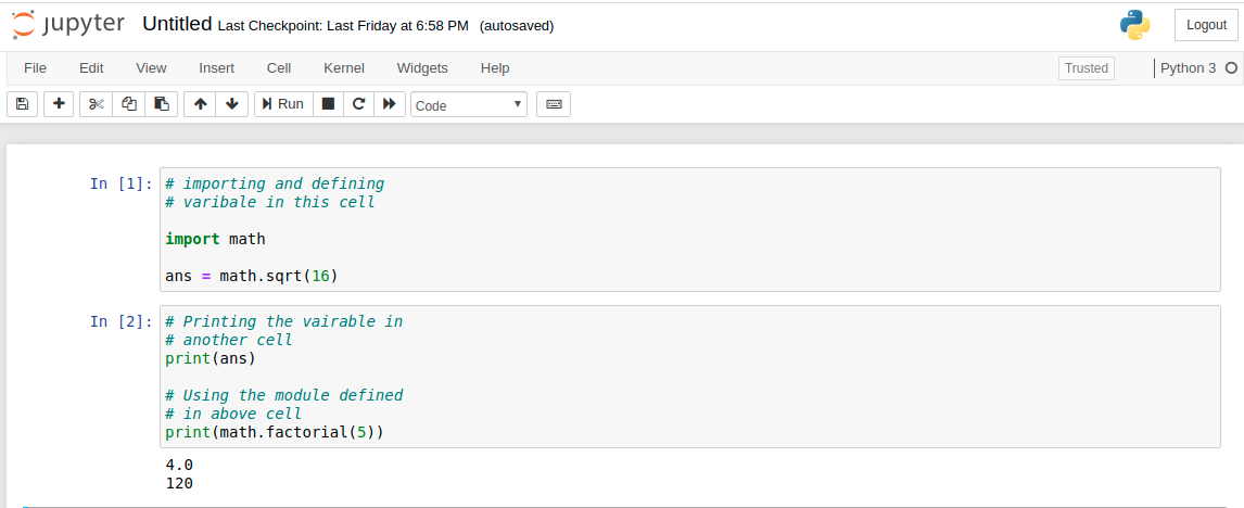 Note: The order of execution of each cell is stated to the left of the cell. In the above example, the cell with In[1] is executed first then the cell with In[2] is executed. Options for kernels: Jupyter Notebook provides various options for kernels. This can be useful if you want to reset things. The options are:
- Restart: This will restart the kernels i.e. clearing all the variables that were defined, clearing the modules that were imported, etc.
- Restart and Clear Output: This will do the same as above but will also clear all the output that was displayed below the cell.
- Restart and Run All: This is also the same as above but will also run all the cells in the top-down order.
- Interrupt: This option will interrupt the kernel execution. It can be useful in the case where the programs continue for execution or the kernel is stuck over some computation.
Naming the notebook
When the notebook is created, Jupyter Notebook names the notebook as Untitled as default. However, the notebook can be renamed. To rename the notebook just click on the word Untitled. This will prompt a dialogue box titled Rename Notebook. Enter the valid name for your notebook in the text bar, then click ok. 
Notebook Extensions
New functionality can be added to Jupyter through extensions. Extensions are javascript module. You can even write your own extension that can access the page’s DOM and the Jupyter Javascript API. Jupyter supports four types of extensions.
- Kernel
- IPyhton Kernel
- Notebook
- Notebook server
Installing Extensions
Most of the extensions can be installed using Python’s pip tool. If an extension can not be installed using pip, then install the extension using the below command.
jupyter nbextension install extension_name
The above only installs the extension but does not enables it. To enable it type the below command in the terminal.
jupyter nbextension enable extension_name
Last Updated :
28 Mar, 2022
Like Article
Save Article
Jupyter Notebook — это мощный инструмент для разработки и представления проектов Data Science в интерактивном виде. Он объединяет код и вывод все в виде одного документа, содержащего текст, математические уравнения и визуализации.
Такой пошаговый подход обеспечивает быстрый, последовательный процесс разработки, поскольку вывод для каждого блока показывается сразу же. Именно поэтому инструмент стал настолько популярным в среде Data Science за последнее время. Большая часть Kaggle Kernels (работы участников конкурсов на платформе Kaggle) сегодня созданы с помощью Jupyter Notebook.

Этот материал предназначен для новичков, которые только знакомятся с Jupyter Notebook, и охватывает все этапы работы с ним: установку, азы использования и процесс создания интерактивного проекта Data Science.
Чтобы начать работать с Jupyter Notebook, библиотеку Jupyter необходимо установить для Python. Проще всего это сделать с помощью pip:
pip3 install jupyter
Лучше использовать pip3, потому что pip2 работает с Python 2, поддержка которого прекратится уже 1 января 2020 года.
Теперь нужно разобраться с тем, как пользоваться библиотекой. С помощью команды cd в командной строке (в Linux и Mac) в первую очередь нужно переместиться в папку, в которой вы планируете работать. Затем запустите Jupyter с помощью следующей команды:
jupyter notebook
Это запустит сервер Jupyter, а браузер откроет новую вкладку со следующим URL: https://localhost:8888/tree. Она будет выглядеть приблизительно вот так:

Отлично. Сервер Jupyter работает. Теперь пришло время создать первый notebook и заполнять его кодом.
Основы Jupyter Notebook
Для создания notebook выберите «New» в верхнем меню, а потом «Python 3». Теперь страница в браузере будет выглядеть вот так:

Обратите внимание на то, что в верхней части страницы, рядом с логотипом Jupyter, есть надпись Untitled — это название notebook. Его лучше поменять на что-то более понятное. Просто наведите мышью и кликните по тексту. Теперь можно выбрать новое название. Например, George's Notebook.
Теперь напишем какой-нибудь код!
Перед первой строкой написано In []. Это ключевое слово значит, что дальше будет ввод. Попробуйте написать простое выражение вывода. Не забывайте, что нужно пользоваться синтаксисом Python 3. После этого нажмите «Run».

Вывод должен отобразиться прямо в notebook. Это и позволяет заниматься программированием в интерактивном формате, имея возможность отслеживать вывод каждого шага.
Также обратите внимание на то, что In [] изменилась и вместе нее теперь In [1]. Число в скобках означает порядок, в котором эта ячейка будет запущена. В первой цифра 1, потому что она была первой запущенной ячейкой. Каждую ячейку можно запускать индивидуально и цифры в скобках будут менять соответственно.
Рассмотрим пример. Настроим 2 ячейки, в каждой из которых будет разное выражение print. Сперва запустим вторую, а потом первую. Можно увидеть, как в результате цифры в скобках меняются.

Если есть несколько ячеек, то между ними можно делиться переменными и импортами. Это позволяет проще разбивать весь код на связанные блоки, не создавая переменную каждый раз. Главное убедиться в запуске ячеек в правильном порядке, чтобы переменные не использовались до того, как были созданы.
Добавление описания к notebook
В Jupyter Notebook есть несколько инструментов, используемых для добавления описания. С их помощью можно не только оставлять комментарии, но также добавлять заголовки, списки и форматировать текст. Это делается с помощью Markdown.
Первым делом нужно поменять тип ячейки. Нажмите на выпадающее меню с текстом «Code» и выберите «Markdown». Это поменяет тип ячейки.
Попробуем несколько вариантов. Заголовки можно создавать с помощью символа #. Один такой символ создаст самый крупный заголовок верхнего уровня. Чем больше #, тем меньше будет текст.
Сделать текст курсивным можно с помощью символов * с двух сторон текста. Если с каждой стороны добавить по два *, то текст станет полужирным. Список создается с помощью тире и пробела для каждого пункта.

Интерактивная наука о данных
Соорудим простой пример проекта Data Science. Этот notebook и код взяты из реального проекта.
Начнем с ячейки Markdown с самым крупным текстом, который делается с помощью одного #. Затем список и описание всех библиотек, которые необходимо импортировать.
Следом идет первая ячейка, в которой происходит импорт библиотек. Это стандартный код для Python Data Science с одним исключение: чтобы прямо видеть визуализации Matplotlib в notebook, нужна следующая строчка: %matplotlib inline.

Следом нужно импортировать набор данных из файла CSV и вывести первые 10 пунктов. Обратите внимание, как Jupyter автоматически показывает вывод функции .head() в виде таблицы. Jupyter отлично работает с библиотекой Pandas!

Теперь нарисуем диаграмму прямо в notebook. Поскольку наверху есть строка %matplotlib inline, при написании plt.show() диаграмма будет выводиться в notebook!
Также обратите внимание на то, как переменные из предыдущих ячеек, содержащие данные из CSV-файла, используются в последующих ячейках в том случае, если по отношению к первым была нажата кнопка «Run».

Это простейший способ создания интерактивного проекта Data Science!
Меню
На сервере Jupyter есть несколько меню, с помощью которых от проекта можно получить максимум. С их помощью можно взаимодействовать с notebook, читать документацию популярных библиотек Python и экспортировать проект для последующей демонстрации.
Файл (File): отвечает за создание, копирование, переименование и сохранение notebook в файл. Самый важный пункт в этом разделе — выпадающее меню Download, с помощью которого можно скачать notebook в разных форматах, включая pdf, html и slides для презентаций.
Редактировать (Edit): используется, чтобы вырезать, копировать и вставлять код. Здесь же можно поменять порядок ячеек, что понадобится для демонстрации проекта.
Вид (View): здесь можно настроить способ отображения номеров строк и панель инструментов. Самый примечательный пункт — Cell Toolbar, к каждой ячейке можно добавлять теги, заметки и другие приложения. Можно даже выбрать способ форматирования для ячейки, что потребуется для использования notebook в презентации.
Вставить (Insert): для добавления ячеек перед или после выбранной.
Ячейка (Cell): отсюда можно запускать ячейки в определенном порядке или менять их тип.
Помощь (Help): в этом разделе можно получить доступ к важной документации. Здесь же упоминаются горячие клавиши для ускорения процесса работы. Наконец, тут можно найти ссылки на документацию для самых важных библиотек Python: Numpy, Scipy, Matplotlib и Pandas.
Jupyter Notebook – невероятно мощный инструмент для интерактивной разработки и представления проектов в области наук о данных. В этой статье вы узнаете, как настроить Jupyter Notebooks на локальном компьютере и как начать использовать его в ваших проектах.
Начнем с определения: что такое «notebook» (блокнот)? Блокнот объединяет код и его вывод в единый документ, который объединяет визуализацию, повествовательный текст, математические уравнения и другие мультимедиа. Этот интуитивно понятный рабочий процесс способствует итеративной и быстрой разработке, что делает ноутбуки все более популярным выбором для представления в данных и их анализа.
Лучше всего то, что в рамках проекта с открытым исходным кодом Project Jupyter он полностью бесплатен.
Проект Jupyter является преемником более раннего проекта IPython Notebook, который впервые был опубликован в качестве прототипа в 2010 году. Хотя в Jupyter Notebooks можно использовать с многими разными языками программирования, в этой статье основное внимание будет уделено Python, поскольку он является наиболее распространенный вариантом использования.
Чтобы получить максимальную отдачу от этого урока, вы должны быть знакомы с программированием, особенно с Python и pandas. Тем не менее, если у вас есть опыт работы с другим языком, Python в этой статье не будет слишком сложным, а статья все равно будет вам полезной в настройке Jupyter Notebooks локально. Как вы увидите позже в этой статье, Jupyter Notebooks также может выступать в качестве гибкой платформы для работы с pandas и даже с Python.
В этой статье мы:
- Изучим основы установки Jupyter и создания своего первого ноутбука
- Погрузимся глубже и рассмотрим всю важную терминологию
- Расскажем, как легко можно обмениваться блокнотами и публиковать их в Интернете.
Пример анализа данных в блокноте Jupyter
Сначала мы пройдемся по настройке и анализу примера, чтобы ответить на наш вопрос. Итак, допустим, вы аналитик данных, и вам было поручено выяснить, как исторически менялась прибыль крупнейших компаний в США. У нас для этого будет набор данных о компаниях из списка Fortune 500, охватывающих более 50 лет с момента первой публикации списка в 1955 году, собранных из открытого архива Fortune. Для анализа мы создали CSV файл данных, который вы можете скачать отсюда.
Как мы покажем, ноутбуки Jupyter идеально подходят для этого исследования.
И так, давайте продолжим и установим Jupyter.
Инсталяция
Для новичка проще всего начать работу с Jupyter Notebooks, установив дистрибутив Anaconda. Anaconda является наиболее широко используемым дистрибутивом Python для работы с данными и поставляется с предустановленными наиболее популярными библиотеками и инструментами. Некоторые из крупнейших библиотек Python, включенных в Anaconda, включают NumPy, pandas и Matplotlib, хотя вы можете взглянуть на полный список с более чем 1000+ пакетов. Это позволит вам приступить к работе, без хлопот управления бесчисленными установками или беспокойства о зависимостях и проблемах установки, связанных с ОС.
Чтобы установить Анаконду, просто:
- Загрузите последнюю версию Anaconda для Python 3 (игнорируйте Python 2.7).
- Установите Anaconda, следуя инструкциям на странице загрузки и/или в исполняемом файле.
Если вы более продвинутый пользователь с уже установленным Python и предпочитаете управлять своими пакетами вручную, вы можете просто использовать pip для установки Jupyter Notebooks:
pip3 install jupyter
Создание вашего первого блокнота
В этом разделе мы научимся запускать и сохранять блокноты, познакомиться с их структурой и рассмотрим их интерфейс. Мы познакомимся с некоторыми основными терминами, которые приведут вас к практическому пониманию того, как самостоятельно использовать Jupyter Notebooks, и подготовимся к следующему разделу, в котором описан пример анализа данных и опробуем на практике все, что мы изучаем здесь.
Запуск Jupyter
В Windows вы можете запустить Jupyter с помощью ярлыка, который Anaconda добавляет в ваше меню «Пуск», которое откроет новую вкладку в веб-браузере по умолчанию, и которая должна выглядеть примерно так, как показано на следующем скриншоте

Это пока не блокнот, но не паникуйте! Это панель инструментов ноутбука, специально разработанная для управления ноутбуками Jupyter. Думайте об этом как о панели запуска.
Имейте в виду, что панель управления предоставит вам доступ только к файлам и подпапкам, содержащимся в каталоге запуска Jupyter; однако каталог запуска может быть изменен. Также можно запустить панель мониторинга в любой системе через командную строку (или терминал в системах Unix), введя команду jupyter notebook; в этом случае текущим рабочим каталогом будет каталог запуска.
Проницательный читатель, возможно, заметил, что URL-адрес панели мониторинга похож на http://localhost:8888/tree. Localhost не является веб-сайтом, но указывает, что контент обслуживается с вашего локального компьютера: с вашего собственного компьютера. Ноутбуки и панель инструментов Jupyter – это веб-приложения, и Jupyter запускает локальный веб сервер Python для обслуживания этих приложений в веб-браузере, что делает его практически независимым от платформы и открывает возможности для более удобного обмена в Интернете.
Интерфейс панели управления в основном не требует пояснений – хотя мы вернемся к нему позже. Так чего же мы ждем? Перейдите в папку, в которой вы хотите создать свой первый блокнот, нажмите кнопку «Создать» в правом верхнем углу и выберите «Python 3» (или выбранную вами версию).

Ваш первый блокнот Jupyter откроется в новой вкладке – каждый блокнот использует свою вкладку, поэтому вы можете открывать несколько блокнотов одновременно. Если вы переключитесь обратно на панель инструментов, вы увидите новый файл Untitled.ipynb и зеленый текст, который говорит о том, что ваш ноутбук работает.
Что за файл ipynb?
Будет полезно понять, что это за файл на самом деле. Каждый файл .ipynb представляет собой текстовый файл, который описывает содержимое вашей записной книжки в формате JSON. Каждая ячейка и ее содержимое, включая вложения изображений, которые были преобразованы в строки текста, перечислены в нем вместе с некоторыми метаданными. Вы можете редактировать их самостоятельно – если знаете, что делаете! – выбрав «Edit> Edit Notebook Metadata» в строке меню в записной книжке.
Вы также можете просмотреть содержимое файлов вашей записной книжки, выбрав «Edit» на панели управления, но ключевое слово здесь – «можете»; нет никакой другой причины, кроме любопытства, делать это, если вы действительно не знаете, что делаете.
Интерфейс Notebook
Теперь, когда перед вами открытый блокнот, надеюсь, его интерфейс не будет выглядеть совершенно чуждым; В конце концов, Jupyter – это просто продвинутый текстовый процессор. Почему бы не осмотреться? Просотрите меню, чтобы почувствовать его, особенно потратьте несколько минут, чтобы прокрутить список команд в палитре команд, который представляет собой небольшую кнопку со значком клавиатуры (или Ctrl + Shift + P).

Вы должны заметить два довольно важных термина, которые, вероятно, являются новыми для вас: cells (ячейки) и kernels (ядра) являются ключом как к пониманию Jupyter, так и к тому, что делает его не просто текстовым процессором. К счастью, эти термины не сложно понять.
- kernel (Ядро) – это «вычислительный движок», который выполняет код, содержащийся в документе ноутбука.
- cell (Ячейка) – это контейнер для текста, который будет отображаться в записной книжке, или код, который будет выполняться ядром записной книжки.
Ячейки (Cell)
Мы вернемся к ядрам чуть позже, но сначала давайте разберемся с ячейками. Ячейки образуют структуру ноутбука. На скриншоте нового блокнота в приведенном выше разделе это поле с зеленым контуром. Есть два основных типа ячеек, которые мы рассмотрим:
- Ячейка кода содержит код, который должен быть выполнен в ядре, и отображает его вывод ниже.
- Ячейка Markdown содержит текст, отформатированный с использованием Markdown, и отображает его вывод на месте при запуске.

Первая ячейка в новой записной книжке всегда является ячейкой кода. Давайте проверим это на классическом примере с Hello World. Введите print (‘Hello World!’) в ячейку и нажмите кнопку запуска на панели инструментов показанная выше или нажмите Ctrl + Enter. Результат должен выглядеть как то так:
print('Hello World!')
Hello World!
Когда вы запустите ячейку, ее вывод будет отображен ниже, а метка слева изменится с In [] на In [1]. Вывод ячейки кода также является частью документа, поэтому вы можете увидеть его в этой статье. Вы всегда можете определить разницу между кодом и ячейками Markdown, потому что ячейки кода имеют эту метку слева, а ячейки Markdown – нет.
Часть «In» метки просто короткая запись слова «Input», а номер метки указывает, когда ячейка была выполнена в ядре – в нашем случае ячейка была выполнена первой. Запустите ячейку снова, и метка изменится на In [2], потому что теперь ячейка была второй, запущенной в ядре. Позже станет понятнее, почему это так полезно, когда мы поближе познакомимся с ядрами.
В строке меню нажмите Insert (Вставить) и выберите Insert Cell Below (Вставить ячейку ниже), чтобы создать новую ячейку кода под первым и попробуйте следующий код, чтобы увидеть, что происходит. Вы замечаете что-то другое?
import time
time.sleep(3)
Эта ячейка не производит никакого вывода, но для ее выполнения требуется три секунды. Обратите внимание, как Jupyter показывает, что ячейка в данный момент работает, изменив метку на In [*].
Как правило, выходные данные ячейки поступают из любых текстовых данных, специально напечатанных во время выполнения ячеек, а также из значения последней строки в ячейке, будь то переменная-одиночка, вызов функции или что-то еще. Например:
def say_hello(recipient):
    return 'Hello, {}!'.format(recipient)
say_hello('Tim')
'Hello, Tim!'
Горячие клавиши
Последнее, что вы, возможно, заметили при запуске ваших ячеек, это то, что их рамка стала синей, тогда как она была зеленой, когда вы редактировали ее. Всегда есть одна «активная» ячейка, выделенная рамкой, цвет которой обозначает ее текущий режим, где зеленый означает edit mode (режим редактирования), а синий – command mode (командный режим).
До сих пор мы показали, как запустить ячейку с помощью Ctrl + Enter, но есть еще много других возможностей. Сочетания клавиш являются очень популярным аспектом среды Jupyter, поскольку они обеспечивают быстрый рабочий процесс на основе ячеек. Многие из этих действий вы можете выполнять в активной ячейке, когда она находится в командном режиме.
Ниже вы найдете список некоторых сочетаний клавиш Jupyter. Вам не нужно сразу их запоминать, но список должен дать вам хорошее представление о том, что это возможно.
- Переключение между режимом редактирования и командным режимом с помощью Esc и Enter соответственно.
- В командном режиме:
- Прокрутите свои ячейки вверх и вниз с помощью клавиш «Вверх» и «Вниз».
- Нажмите A или B, чтобы вставить новую ячейку выше или ниже активной ячейки.
- M преобразует активную ячейку в ячейку Markdown.
- Y установит активную ячейку в кодовую ячейку.
- D + D (D дважды) удалит активную ячейку.
- Z отменит удаление ячейки.
- Удерживайте Shift и нажмите Вверх или Вниз, чтобы выбрать несколько ячеек одновременно.
- С выделением нескольких ячеек Shift + M объединит выбранные ячейки.
- Ctrl + Shift + – в режиме редактирования разделит активную ячейку по курсору.
- Вы также можете нажать и Shift + клик на полях слева от ваших ячеек, чтобы выбрать их.
Попробуй это в своей записной книжке. После того, как вы опробуете все команды, создайте новую ячейку Markdown, и мы научимся форматировать текст в наших блокнотах.
Markdown
Markdown – это легкий, простой в освоении язык разметки для форматирования простого текста. Его синтаксис имеет однозначное соответствие с тегами HTML, поэтому некоторые предварительные знания здесь могут быть полезны, но это определенно не является обязательным условием. Давайте рассмотрим основы с кратким примером.
# This is a level 1 heading
## This is a level 2 heading
This is some plain text that forms a paragraph.
Add emphasis via **bold** and __bold__, or *italic* and _italic_.
Paragraphs must be separated by an empty line.
* Sometimes we want to include lists.
* Which can be indented.
1. Lists can also be numbered.
2. For ordered lists.
[It is possible to include hyperlinks](https://www.example.com)
Inline code uses single backticks: `foo()`, and code blocks use triple backticks:
```
bar()
```
Or can be indented by 4 spaces:
foo()
And finally, adding images is easy: 
При прикреплении изображений у вас есть три варианта:
- Используйте URL для изображения в Интернете.
- Используйте локальный URL-адрес изображения, которое вы будете хранить рядом с ноутбуком, например, в том же git-репо.
- Добавьте вложение через «Edit> Insert Image»; Это преобразует изображение в строку и сохраняет его в файле .ipynb вашего ноутбука.
- Обратите внимание, что это сделает ваш файл .ipynb намного больше!
У Markdown гораздо больше возможностей, особенно в отношении гиперссылок, а также возможно просто включить простой HTML. Если вы захотите узнать больше, вы можете обратиться к официальному руководству от создателя Markdown, Джона Грубера, на его веб-сайте.
Ядра (Kernels)
За каждым ноутбуком работает ядро. Когда вы запускаете ячейку кода, этот код выполняется в ядре, и любой вывод возвращается обратно в ячейку для отображения. Состояние ядра сохраняется во времени и между ячейками – оно относится к документу в целом, а не к отдельным ячейкам.
Например, если вы импортируете библиотеки или объявляете переменные в одной ячейке, они будут доступны в другой. Таким образом, вы можете думать о документе блокнота как о чем-то сравнимом с файлом сценария, за исключением того, что он является мультимедийным. Давайте попробуем, чтобы почувствовать это. Сначала мы импортируем пакет Python и определим функцию.
import numpy as np
def square(x):
    return x * x
Как только мы выполнили ячейку выше, мы можем ссылаться на np и square в любой другой ячейке.
x = np.random.randint(1, 10)
y = square(x)
print('%d squared is %d' % (x, y))
1 squared is 1
Это будет работать независимо от порядка ячеек в вашем блокноте. Вы можете попробовать сами, давайте снова распечатаем наши переменные.
print('Is %d squared is %d?' % (x, y))
Is 1 squared is 1?
Здесь нет сюрпризов! Но теперь давайте изменим у.
y = 10
Как вы думаете, что произойдет, если мы снова запустим ячейку, содержащую наш оператор print? Мы получим на выходе 4 в квадрате 10?
Большую часть времени поток в вашем ноутбуке будет сверху вниз, но часто приходится возвращаться, чтобы внести изменения. В этом случае важен порядок выполнения, указанный слева от каждой ячейки, например, In [6], позволит вам узнать, имеет ли какая-либо из ваших ячеек устаревший вывод. И если вы когда-нибудь захотите сбросить настройки, есть несколько невероятно полезных опций из меню Kernel:
- Restart: перезапускает ядро, таким образом очищая все переменные и т.д., которые были определены.
- Restart & Clear Output: то же, что и выше, но также стирает вывод, отображаемый под ячейками кода.
- Restart & Run All: то же, что и выше, но также будет запускать все ваши ячейки в порядке от первого до последнего.
Если ваше ядро зависло в вычислении, и вы хотите остановить его, вы можете выбрать опцию Interupt.
Выбор ядра
Возможно, вы заметили, что Jupyter дает вам возможность сменить ядро, и на самом деле есть много разных вариантов на выбор. Когда вы создавали новую записную книжку на панели инструментов, выбирая версию Python, вы фактически выбирали, какое ядро использовать.
Существуют не только ядра для разных версий Python, но и более 100 языков, включая Java, C и даже Fortran. Исследователи данных могут быть особенно заинтересованы в ядрах для R и Julia, а также в imatlab и ядре Calysto MATLAB Kernel для Matlab. Ядро SoS обеспечивает многоязычную поддержку в пределах одного ноутбука. Каждое ядро имеет свои собственные инструкции по установке, но, вероятно, потребует от вас выполнения некоторых команд на вашем компьютере.
Пример анализа
Теперь когда мы рассмотрели, что такое Jupyter Notebook, пришло время взглянуть на то, как они используются на практике, что должно дать вам более четкое представление о том, почему они так популярны. Наконец-то пришло время начать работу с тем набором данных Fortune 500, который упоминался ранее. Помните, наша цель – узнать, как исторически менялась прибыль крупнейших компаний США.
Названия для ноутбуков
Прежде чем начать создавать свой проект, вы, вероятно, захотите дать ему осмысленное имя. Возможно, это несколько сбивает с толку: но вы не можете назвать или переименовать свои записные книжки из самого приложения для записной книжки, а для переименования файла .ipynb необходимо использовать панель мониторинга или файловый браузер. Мы вернемся к информационной панели, чтобы переименовать созданный ранее файл, который будет иметь имя файла по умолчанию для записной книжки Untitled.ipynb.
Вы не можете переименовать ноутбук во время его работы, потому что его сначала нужно выключить. Самый простой способ сделать это – выбрать «File> Close and Halt» в меню ноутбука. Однако вы также можете выключить ядро, перейдя в «Kernel> Shutdown» в приложении для ноутбука или выбрав ноутбук на приборной панели и нажав «Shutdown» (см. Изображение ниже).

Затем вы можете выбрать свой блокнот и нажать «Rename» на панели управления.

Обратите внимание, что закрытие вкладки «notebook» в вашем браузере не «закроет» вашу записную книжку так же, как закрытие документа в традиционном приложении. Ядро ноутбука будет продолжать работать в фоновом режиме и должно быть отключено, прежде чем оно действительно «закроется». Это очень удобно, если вы случайно закрыли вкладку или браузер! Если ядро закрыто, вы можете закрыть вкладку, не беспокоясь о том, работает ли оно по-прежнему или нет.
Как только вы назвали свою записную книжку, откройте ее снова, и мы начнем.
Настройка
Обычно начинают с ячейки кода, специально предназначенной для импорта и настройки, поэтому, если вы решите добавить или изменить что-либо, вы можете просто отредактировать и повторно запустить ячейку, не вызывая побочных эффектов.
import pandas as pd
import matplotlib.pyplot as plt
import seaborn as sns
sns.set(style="darkgrid")
Здесь мы импортируем pandas для работы с нашими данными, Matplotlib для построения графиков и Seaborn для улучшения внешнего вида наших графиков. Обычно также импортируется NumPy, но в нашем случае, мы используем его через pandas, и нам не нужно это делать явно. Последняя строка не является командой Python, она является нечто, называемое строковой магией, для инструктирования Jupyter захватывать графики Matplotlib и отображать их в выходных данных ячейки; это одна из ряда расширенных функций, которые выходят за рамки данной статьи.
Давайте продолжим и загрузим наши данные.
df = pd.read_csv('fortune500.csv')
Целесообразно делать это в отдельной ячейке на случай, если нам понадобится перезагрузить ее в любой момент.
Сохранение и контрольная точка
Теперь, когда мы начали создавать проект, лучше регулярно сохраняться. Нажатие Ctrl + S сохранит вашу записную книжку, вызвав команду «Save and Checkpoint», но что это за checkpoint (контрольная точка)?
Каждый раз, когда вы создаете новую записную книжку, создается файл контрольной точки, а также файл вашей записной книжки; он будет расположен в скрытом подкаталоге вашего места сохранения с именем .ipynb_checkpoints, и также является файлом .ipynb. По умолчанию Jupyter каждые 120 секунд автоматически сохраняет ваш блокнот в этот файл контрольных точек, не изменяя основной файл блокнота. Когда вы сохраняете и сохраняете контрольную точку, файлы записной книжки и контрольной точки обновляются. Следовательно, контрольная точка позволяет вам восстановить несохраненную работу в случае непредвиденной проблемы. Вы можете вернуться к контрольной точке из меню через «File> Revert to Checkpoint».
Изучение нашего набора данных
Наш блокнот благополучно сохранен, и мы загрузили наш набор данных переменную df в наиболее часто используемую структуру данных pandas, которая называется DataFrame и в основном выглядит как таблица. Давай те посмотрим как выглядят наши данные?
df.head()
| year | rank | company | revenue (in millions) | profit (in millions) | |
|---|---|---|---|---|---|
| 0 | 1955 | 1 | General Motors | 9823.5 | 806 |
| 1 | 1955 | 2 | Exxon Mobil | 5661.4 | 584.8 |
| 2 | 1955 | 3 | U.S. Steel | 3250.4 | 195.4 |
| 3 | 1955 | 4 | General Electric | 2959.1 | 212.6 |
| 4 | 1955 | 5 | Esmark | 2510.8 | 19.1 |
df.tail()
| year | rank | company | revenue (in millions) | profit (in millions) | |
|---|---|---|---|---|---|
| 25495 | 2005 | 496 | Wm. Wrigley Jr. | 3648.6 | 493 |
| 25496 | 2005 | 497 | Peabody Energy | 3631.6 | 175.4 |
| 25497 | 2005 | 498 | Wendy’s International | 3630.4 | 57.8 |
| 25498 | 2005 | 499 | Kindred Healthcare | 3616.6 | 70.6 |
| 25499 | 2005 | 500 | Cincinnati Financial | 3614.0 | 584 |
У нас есть столбцы, которые нам нужны, и каждая строка соответствует одной компании за один год.
Давайте просто переименуем эти столбцы, чтобы мы могли обратиться к ним позже.
df.columns = ['year', 'rank', 'company', 'revenue', 'profit']
Далее нам нужно изучить наш набор данных. Являются ли они завершенными? Распознало ли pandas их, как ожидалось? Отсутствуют ли в них какие-либо значения?
len(df)
25500
У нас есть 500 строк за каждый год с 1955 по 2005 год включительно.
Давайте проверим, был ли наш набор данных импортирован, как мы ожидали. Простая проверка состоит в том, чтобы увидеть, были ли типы данных (или dtypes) правильно интерпретированы.
df.dtypes
year int64
rank int64
company object
revenue float64
profit object
dtype: object
Ооо Похоже, что с колонкой profit что-то не так – мы ожидаем, что это будет float64, как колонка revenue. Это указывает на то, что она, вероятно, содержит нецелые значения, так что давайте посмотрим.
non_numberic_profits = df.profit.str.contains('[^0-9.-]')
df.loc[non_numberic_profits].head()
| year | rank | company | revenue | profit | |
|---|---|---|---|---|---|
| 228 | 1955 | 229 | Norton | 135.0 | N.A. |
| 290 | 1955 | 291 | Schlitz Brewing | 100.0 | N.A. |
| 294 | 1955 | 295 | Pacific Vegetable Oil | 97.9 | N.A. |
| 296 | 1955 | 297 | Liebmann Breweries | 96.0 | N.A. |
| 352 | 1955 | 353 | Minneapolis-Moline | 77.4 | N.A. |
Как мы и подозревали! Некоторые значения являются строками, которые использовались для указания отсутствующих данных. Есть ли какие-то другие значения, которые закрались?
set(df.profit[non_numberic_profits])
{'N.A.'}
Получается, что других значений нет. Это облегчает интерпретацию, но что нам делать? Это зависит от того, сколько значений пропущено.
len(df.profit[non_numberic_profits])
369
Это небольшая часть нашего набора данных, хотя и не совсем несущественная, поскольку все еще составляет около 1,5%. Если строки, содержащие N.A., примерно одинаково распределены по годам, самым простым решением было бы просто удалить их. Итак, давайте кратко рассмотрим их распределение.
bin_sizes, _, _ = plt.hist(df.year[non_numberic_profits], bins=range(1955, 2006))

На первый взгляд, мы видим, что самые недопустимые значения за один год составляют менее 25, а поскольку существует 500 точек данных в год, удаление этих значений будет составлять менее 4% данных для худших лет. Действительно, кроме всплеска около 90-х годов, большинство лет имеют менее половины недостающих значений пика. Для наших целей допустим, что это приемлемо, и мы просто удалим эти строки.
df = df.loc[~non_numberic_profits]
df.profit = df.profit.apply(pd.to_numeric)
Мы должны проверить, что у нас получилось.
len(df)
25131
df.dtypes
year int64
rank int64
company object
revenue float64
profit float64
dtype: object
Супер! Мы завершили настройку набора данных.
Если бы вы собирались представить свою записную книжку в виде отчета, вы могли бы избавиться от созданных нами исследовательских ячеек, которые включены здесь в качестве демонстрации процесса работы с записными книжками, и объединить соответствующие ячейки (см. Раздел «Дополнительные функции» ниже для подробностей об этом) для создания единой ячейки настройки набора данных. Это будет означать, что если мы когда-нибудь испортим наш набор данных в другом месте, мы сможем просто повторно запустить ячейку настройки, чтобы восстановить ее.
Графики с matplotlib
Далее мы можем перейти к решению данного вопроса, построив график средней прибыли за год. Мы можем также рассчитать доход, поэтому сначала мы определим некоторые переменные и метод, чтобы уменьшить наш код.
group_by_year = df.loc[:, ['year', 'revenue', 'profit']].groupby('year')

avgs = group_by_year.mean()
x = avgs.index
y1 = avgs.profit

def plot(x, y, ax, title, y_label):
    ax.set_title(title)
    ax.set_ylabel(y_label)
    ax.plot(x, y)
    ax.margins(x=0, y=0)
Теперь график!
fig, ax = plt.subplots()
plot(x, y1, ax, 'Increase in mean Fortune 500 company profits from 1955 to 2005', 'Profit (millions)')

Вау, это похоже на экспоненту, но у нее есть огромные провалы. Они должны соответствовать рецессии начала 1990-х и пузырю доткомов. Это довольно интересно увидеть в данных. Но почему прибыль возвращается к еще более высоким уровням после каждой рецессии?
Может быть, доходы могут рассказать нам больше.
y2 = avgs.revenue
fig, ax = plt.subplots()
plot(x, y2, ax, 'Increase in mean Fortune 500 company revenues from 1955 to 2005', 'Revenue (millions)')

Это добавляет другую сторону истории. Доходы отнюдь не так сильно пострадали, это отличная бухгалтерская работа для финансовых отделов.
С небольшой помощью Stack Overflow мы можем наложить эти графики с +/- их стандартными отклонениями.
def plot_with_std(x, y, stds, ax, title, y_label):
    ax.fill_between(x, y - stds, y + stds, alpha=0.2)
    plot(x, y, ax, title, y_label)

fig, (ax1, ax2) = plt.subplots(ncols=2)
title = 'Increase in mean and std Fortune 500 company %s from 1955 to 2005'
stds1 = group_by_year.std().profit.values
stds2 = group_by_year.std().revenue.values

plot_with_std(x, y1.values, stds1, ax1, title % 'profits', 'Profit (millions)')
plot_with_std(x, y2.values, stds2, ax2, title % 'revenues', 'Revenue (millions)')

fig.set_size_inches(14, 4)
fig.tight_layout()

Это ошеломляет, стандартные отклонения огромны. Некоторые компании из списка Fortune 500 зарабатывают миллиарды, в то время как другие теряют миллиарды, и риск увеличивается вместе с ростом прибыли за последние годы. Возможно, некоторые компании работают лучше, чем другие; Являются ли прибыли первых 10% более или менее волатильными, чем нижние 10%?
Есть много вопросов, которые мы могли бы рассмотреть далее, и легко увидеть, как процесс работы в блокноте соответствует собственному мыслительному процессу, поэтому сейчас пришло время подвести этот пример к концу. Этот блокнот помог нам легко исследовать наш набор данных в одном месте без переключения контекста между приложениями, и наша работа сразу становится доступной и воспроизводимой. Если бы мы хотели создать более краткий отчет для конкретной аудитории, мы могли бы быстро реорганизовать нашу работу, объединив ячейки и удалив промежуточный код.
Примечание: оригинальная версия этой статьи использовала as_matrix () вместо .values в приведенном выше фрагменте кода. На момент написания этой статьи команда .as_matrix () все еще существует, но ее планируется удалить в будущей версии pandas, поэтому мы заменили его на значение .values.
Делимся своими ноутбуками
Когда люди говорят о совместном использовании своих ноутбуков, обычно они рассматривают две парадигмы. Чаще всего люди разделяют конечный результат своей работы, что означает обмен неинтерактивными, предварительно отрендеренными версиями своих ноутбуков; однако также существует возможность совместного использования ноутбуков с такими вспомогательными системами контроля версий, как Git.
Так же, в интернете появляются новые компании, предлагающие возможность запуска интерактивных Jupyter Notebooks в облаке.
Прежде чем поделиться
Общий блокнот будет отображаться точно в том состоянии, в котором он находился при экспорте или сохранении, включая вывод любых ячеек кода. Поэтому, чтобы обеспечить совместимость вашего ноутбука, так сказать, есть несколько шагов, которые вы должны предпринять, прежде чем им делиться:
- Кликните “Cell > All Output > Clear”
- Кликните “Kernel > Restart & Run All”
- Дождитесь окончания выполнения ваших ячеек кода и проверьте, что они отработали так, как ожидалось.
Это гарантирует, что ваши записные книжки не будут содержать промежуточный вывод, не будут иметь устаревшее состояние и будут выполнены в порядке на момент публикации.
Экспорт ваших ноутбуков
Jupyter имеет встроенную поддержку экспорта в HTML и PDF, а также в некоторые другие форматы, которые вы можете найти в меню «File> Download As». Если вы хотите поделиться своими записными книжками с небольшой частной группой, этой функция будет достаточно. Но если совместного доступа к экспортированным файлам будет не достаточно, есть также несколько чрезвычайно популярных методов совместного использования файлов .ipynb в Интернете.
GitHub
Поскольку к началу 2018 года количество общедоступных ноутбуков на GitHub превысило 1,8 миллиона, это, безусловно, самая популярная независимая платформа для обмена проектами Jupyter со всем миром. GitHub имеет встроенную поддержку рендеринга файлов .ipynb непосредственно как в репозиториях, так и в списках на своем веб-сайте. Если вы еще не знаете, GitHub – это платформа для размещения кода для контроля версий и совместной работы для репозиториев, созданных с помощью Git. Вам понадобится аккаунт, чтобы воспользоваться их услугами (стандартные аккаунты бесплатны).
Если у вас есть учетная запись GitHub, самый простой способ поделиться записной книжкой через GitHub на самом деле вообще не используя Git. С 2008 года GitHub предоставляет сервис Gist для размещения и совместного использования фрагментов кода, каждый из которых имеет свой собственный репозиторий. Чтобы поделиться блокнотом с помощью Gists:
- Войдите в GitHub и перейдите на gist.github.com.
- Откройте файл .ipynb в текстовом редакторе, выберите его содержимое и скопируйте JSON в память.
- Вставьте скопированное в блокнот JSON в gist.
- Определите имя файла вашего Gist, не забывая добавить .iypnb, иначе это не сработает.
- Нажмите “Create secret gist” или “Create public gist.”
Это должно выглядеть примерно так:

Если вы создали общедоступную Gist, теперь вы сможете поделиться ее URL-адресом с кем угодно, а другие смогут fork and clone вашу работу.
Создание собственного репозитория Git и распространение его на GitHub выходит за рамки данного руководства, но GitHub предоставляет множество руководств, которые помогут вам освоить его самостоятельно.
Дополнительным советом для тех, кто использует git, является добавление исключения в ваш .gitignore для скрытых каталогов .ipynb_checkpoints, которые создает Jupyter, чтобы избежать ненужной фиксации файлов контрольных точек в вашем репо.
Nbviewer
К 2015 году NBViewer стал самым популярным средством рендеринга ноутбуков в Интернете. Если у вас уже есть место для размещения ваших ноутбуков Jupyter в Интернете, будь то GitHub или где-либо еще, NBViewer отобразит ваш блокнот и предоставит совместно используемый URL-адрес вместе с ним. Предоставляется как бесплатный сервис в рамках проекта Jupyter, он доступен по адресу nbviewer.jupyter.org.
Первоначально разработанный до интеграции GitHub с Jupyter Notebook, NBViewer позволяет любому вводить URL-адрес, идентификатор Gist или имя пользователя/репозиторий/файл GitHub, и он отображает блокнот в виде веб-страницы. Идентификатор Gist – это уникальный номер в конце URL; например, строка символов после последнего обратного слеша в https://gist.github.com/username/50896401c23e0bf417e89cd57e89e1de. Если вы введете имя пользователя GitHub или username/репо, вы увидите минимальный файловый браузер, который позволит вам просматривать репозитории пользователя и их содержимое.
URL-адрес, отображаемый NBViewer при отображении записной книжки, является константой в зависимости от URL-адреса записываемой записной книжки, поэтому вы можете поделиться этим с кем угодно, и он будет работать, пока исходные файлы остаются в сети.
Заключение
Начав с основ, мы познакомились с естественным рабочим процессом Jupyter Notebooks, углубились в более продвинутые функции IPython и, наконец, научились делиться своей работой с друзьями, коллегами и миром. И мы сделали все это из самой записной книжки!
Если вы хотите получить вдохновение для своих собственных ноутбуков, Jupyter собрал галерею интересных ноутбуков Jupyter, которые вам могут пригодиться, и на домашней странице Nbviewer есть ссылки на действительно интересные примеры качественных ноутбуков.
Оригинальная статья: Jupyter Notebook for Beginners: A Tutorial
Была ли вам полезна эта статья?
What is Jupyter Notebook?
The Jupyter Notebook is an incredibly powerful tool for interactively developing and presenting data science projects. This article will walk you through how to use Jupyter Notebooks for data science projects and how to set it up on your local machine.
First, though: what is a “notebook”?
A notebook integrates code and its output into a single document that combines visualizations, narrative text, mathematical equations, and other rich media. In other words: it’s a single document where you can run code, display the output, and also add explanations, formulas, charts, and make your work more transparent, understandable, repeatable, and shareable.
Using Notebooks is now a major part of the data science workflow at companies across the globe. If your goal is to work with data, using a Notebook will speed up your workflow and make it easier to communicate and share your results.
Best of all, as part of the open source Project Jupyter, Jupyter Notebooks are completely free. You can download the software on its own, or as part of the Anaconda data science toolkit.
Although it is possible to use many different programming languages in Jupyter Notebooks, this article will focus on Python, as it is the most common use case. (Among R users, R Studio tends to be a more popular choice).
How to Follow This Tutorial
To get the most out of this tutorial you should be familiar with programming — Python and pandas specifically. That said, if you have experience with another language, the Python in this article shouldn’t be too cryptic, and will still help you get Jupyter Notebooks set up locally.
Jupyter Notebooks can also act as a flexible platform for getting to grips with pandas and even Python, as will become apparent in this tutorial.
We will:
- Cover the basics of installing Jupyter and creating your first notebook
- Delve deeper and learn all the important terminology
- Explore how easily notebooks can be shared and published online.
(In fact, this article was written as a Jupyter Notebook! It’s published here in read-only form, but this is a good example of how versatile notebooks can be. In fact, most of our programming tutorials and even our Python courses were created using Jupyter Notebooks).
Example Data Analysis in a Jupyter Notebook
First, we will walk through setup and a sample analysis to answer a real-life question. This will demonstrate how the flow of a notebook makes data science tasks more intuitive for us as we work, and for others once it’s time to share our work.
So, let’s say you’re a data analyst and you’ve been tasked with finding out how the profits of the largest companies in the US changed historically. You find a data set of Fortune 500 companies spanning over 50 years since the list’s first publication in 1955, put together from Fortune’s public archive. We’ve gone ahead and created a CSV of the data you can use here.
As we shall demonstrate, Jupyter Notebooks are perfectly suited for this investigation. First, let’s go ahead and install Jupyter.
Installation
The easiest way for a beginner to get started with Jupyter Notebooks is by installing Anaconda.
Anaconda is the most widely used Python distribution for data science and comes pre-loaded with all the most popular libraries and tools.
Some of the biggest Python libraries included in Anaconda include NumPy, pandas, and Matplotlib, though the full 1000+ list is exhaustive.
Anaconda thus lets us hit the ground running with a fully stocked data science workshop without the hassle of managing countless installations or worrying about dependencies and OS-specific (read: Windows-specific) installation issues.
To get Anaconda, simply:
- Download the latest version of Anaconda for Python 3.8.
- Install Anaconda by following the instructions on the download page and/or in the executable.
If you are a more advanced user with Python already installed and prefer to manage your packages manually, you can just use pip:
pip3 install jupyterCreating Your First Notebook
In this section, we’re going to learn to run and save notebooks, familiarize ourselves with their structure, and understand the interface. We’ll become intimate with some core terminology that will steer you towards a practical understanding of how to use Jupyter Notebooks by yourself and set us up for the next section, which walks through an example data analysis and brings everything we learn here to life.
Running Jupyter
On Windows, you can run Jupyter via the shortcut Anaconda adds to your start menu, which will open a new tab in your default web browser that should look something like the following screenshot.
This isn’t a notebook just yet, but don’t panic! There’s not much to it. This is the Notebook Dashboard, specifically designed for managing your Jupyter Notebooks. Think of it as the launchpad for exploring, editing and creating your notebooks.
Be aware that the dashboard will give you access only to the files and sub-folders contained within Jupyter’s start-up directory (i.e., where Jupyter or Anaconda is installed). However, the start-up directory can be changed.
It is also possible to start the dashboard on any system via the command prompt (or terminal on Unix systems) by entering the command jupyter notebook; in this case, the current working directory will be the start-up directory.
With Jupyter Notebook open in your browser, you may have noticed that the URL for the dashboard is something like https://localhost:8888/tree. Localhost is not a website, but indicates that the content is being served from your local machine: your own computer.
Jupyter’s Notebooks and dashboard are web apps, and Jupyter starts up a local Python server to serve these apps to your web browser, making it essentially platform-independent and opening the door to easier sharing on the web.
(If you don’t understand this yet, don’t worry — the important point is just that although Jupyter Notebooks opens in your browser, it’s being hosted and run on your local machine. Your notebooks aren’t actually on the web until you decide to share them.)
The dashboard’s interface is mostly self-explanatory — though we will come back to it briefly later. So what are we waiting for? Browse to the folder in which you would like to create your first notebook, click the “New” drop-down button in the top-right and select “Python 3”:
Hey presto, here we are! Your first Jupyter Notebook will open in new tab — each notebook uses its own tab because you can open multiple notebooks simultaneously.
If you switch back to the dashboard, you will see the new file Untitled.ipynb and you should see some green text that tells you your notebook is running.
What is an ipynb File?
The short answer: each .ipynb file is one notebook, so each time you create a new notebook, a new .ipynb file will be created.
The longer answer: Each .ipynb file is a text file that describes the contents of your notebook in a format called JSON. Each cell and its contents, including image attachments that have been converted into strings of text, is listed therein along with some metadata.
You can edit this yourself — if you know what you are doing! — by selecting “Edit > Edit Notebook Metadata” from the menu bar in the notebook. You can also view the contents of your notebook files by selecting “Edit” from the controls on the dashboard
However, the key word there is can. In most cases, there’s no reason you should ever need to edit your notebook metadata manually.
The Notebook Interface
Now that you have an open notebook in front of you, its interface will hopefully not look entirely alien. After all, Jupyter is essentially just an advanced word processor.
Why not take a look around? Check out the menus to get a feel for it, especially take a few moments to scroll down the list of commands in the command palette, which is the small button with the keyboard icon (or Ctrl + Shift + P).
There are two fairly prominent terms that you should notice, which are probably new to you: cells and kernels are key both to understanding Jupyter and to what makes it more than just a word processor. Fortunately, these concepts are not difficult to understand.
- A kernel is a “computational engine” that executes the code contained in a notebook document.
- A cell is a container for text to be displayed in the notebook or code to be executed by the notebook’s kernel.
Cells
We’ll return to kernels a little later, but first let’s come to grips with cells. Cells form the body of a notebook. In the screenshot of a new notebook in the section above, that box with the green outline is an empty cell. There are two main cell types that we will cover:
- A code cell contains code to be executed in the kernel. When the code is run, the notebook displays the output below the code cell that generated it.
- A Markdown cell contains text formatted using Markdown and displays its output in-place when the Markdown cell is run.
The first cell in a new notebook is always a code cell.
Let’s test it out with a classic hello world example: Type print('Hello World!') into the cell and click the run button  in the toolbar above or press
 Ctrl + Enter.
The result should look like this:
print('Hello World!')Hello World!When we run the cell, its output is displayed below and the label to its left will have changed from In [ ] to In [1].
The output of a code cell also forms part of the document, which is why you can see it in this article. You can always tell the difference between code and Markdown cells because code cells have that label on the left and Markdown cells do not.
The “In” part of the label is simply short for “Input,” while the label number indicates when the cell was executed on the kernel — in this case the cell was executed first.
Run the cell again and the label will change to In [2] because now the cell was the second to be run on the kernel. It will become clearer why this is so useful later on when we take a closer look at kernels.
From the menu bar, click Insert and select Insert Cell Below to create a new code cell underneath your first and try out the following code to see what happens. Do you notice anything different?
import time
time.sleep(3)
This cell doesn’t produce any output, but it does take three seconds to execute. Notice how Jupyter signifies when the cell is currently running by changing its label to In [*].
In general, the output of a cell comes from any text data specifically printed during the cell’s execution, as well as the value of the last line in the cell, be it a lone variable, a function call, or something else. For example:
def say_hello(recipient):
    return 'Hello, {}!'.format(recipient)

say_hello('Tim')
'Hello, Tim!'You’ll find yourself using this almost constantly in your own projects, and we’ll see more of it later on.
Keyboard Shortcuts
One final thing you may have observed when running your cells is that their border turns blue, whereas it was green while you were editing. In a Jupyter Notebook, there is always one “active” cell highlighted with a border whose color denotes its current mode:
- Green outline — cell is in «edit mode»
- Blue outline — cell is in «command mode»
So what can we do to a cell when it’s in command mode? So far, we have seen how to run a cell with Ctrl + Enter, but there are plenty of other commands we can use. The best way to use them is with keyboard shortcuts
Keyboard shortcuts are a very popular aspect of the Jupyter environment because they facilitate a speedy cell-based workflow. Many of these are actions you can carry out on the active cell when it’s in command mode.
Below, you’ll find a list of some of Jupyter’s keyboard shortcuts. You don’t need to memorize them all immediately, but this list should give you a good idea of what’s possible.
- Toggle between edit and command mode with
EscandEnter, respectively. - Once in command mode:
- Scroll up and down your cells with your
UpandDownkeys. - Press
AorBto insert a new cell above or below the active cell. Mwill transform the active cell to a Markdown cell.Ywill set the active cell to a code cell.D + D(Dtwice) will delete the active cell.Zwill undo cell deletion.- Hold
Shiftand pressUporDownto select multiple cells at once. With multiple cells selected,Shift + Mwill merge your selection.
- Scroll up and down your cells with your
Ctrl + Shift + -, in edit mode, will split the active cell at the cursor.- You can also click and
Shift + Clickin the margin to the left of your cells to select them.
Go ahead and try these out in your own notebook. Once you’re ready, create a new Markdown cell and we’ll learn how to format the text in our notebooks.
Markdown
Markdown is a lightweight, easy to learn markup language for formatting plain text. Its syntax has a one-to-one correspondence with HTML tags, so some prior knowledge here would be helpful but is definitely not a prerequisite.
Remember that this article was written in a Jupyter notebook, so all of the narrative text and images you have seen so far were achieved writing in Markdown. Let’s cover the basics with a quick example:
# This is a level 1 heading
## This is a level 2 heading
This is some plain text that forms a paragraph. Add emphasis via **bold** and __bold__, or *italic* and _italic_.
Paragraphs must be separated by an empty line.
* Sometimes we want to include lists.
* Which can be bulleted using asterisks.
1. Lists can also be numbered.
2. If we want an ordered list.
[It is possible to include hyperlinks](https://www.example.com)
Inline code uses single backticks: foo(), and code blocks use triple backticks:
```
bar()
```
Or can be indented by 4 spaces:
foo()
And finally, adding images is easy: Here’s how that Markdown would look once you run the cell to render it:

(Note that the alt text for the image is displayed here because we didn’t actually use a valid image URL in our example)
When attaching images, you have three options:
- Use a URL to an image on the web.
- Use a local URL to an image that you will be keeping alongside your notebook, such as in the same git repo.
- Add an attachment via “Edit > Insert Image”; this will convert the image into a string and store it inside your notebook
.ipynbfile. Note that this will make your.ipynbfile much larger!
There is plenty more to Markdown, especially around hyperlinking, and it’s also possible to simply include plain HTML. Once you find yourself pushing the limits of the basics above, you can refer to the official guide from Markdown’s creator, John Gruber, on his website.
Kernels
Behind every notebook runs a kernel. When you run a code cell, that code is executed within the kernel. Any output is returned back to the cell to be displayed. The kernel’s state persists over time and between cells — it pertains to the document as a whole and not individual cells.
For example, if you import libraries or declare variables in one cell, they will be available in another. Let’s try this out to get a feel for it. First, we’ll import a Python package and define a function:
import numpy as np
def square(x):
    return x * x
Once we’ve executed the cell above, we can reference np and square in any other cell.
x = np.random.randint(1, 10)
y = square(x)
print('%d squared is %d' % (x, y))
1 squared is 1This will work regardless of the order of the cells in your notebook. As long as a cell has been run, any variables you declared or libraries you imported will be available in other cells.
You can try it yourself, let’s print out our variables again.
print('Is %d squared %d?' % (x, y))Is 1 squared 1?No surprises here! But what happens if we change the value of y?
y = 10
print('Is %d squared is %d?' % (x, y))
If we run the cell above, what do you think would happen?
We will get an output like: Is 4 squared 10?. This is because once we’ve run the y = 10 code cell, y is no longer equal to the square of x in the kernel.
Most of the time when you create a notebook, the flow will be top-to-bottom. But it’s common to go back to make changes. When we do need to make changes to an earlier cell, the order of execution we can see on the left of each cell, such as In [6], can help us diagnose problems by seeing what order the cells have run in.
And if we ever wish to reset things, there are several incredibly useful options from the Kernel menu:
- Restart: restarts the kernel, thus clearing all the variables etc that were defined.
- Restart & Clear Output: same as above but will also wipe the output displayed below your code cells.
- Restart & Run All: same as above but will also run all your cells in order from first to last.
If your kernel is ever stuck on a computation and you wish to stop it, you can choose the Interrupt option.
Choosing a Kernel
You may have noticed that Jupyter gives you the option to change kernel, and in fact there are many different options to choose from. Back when you created a new notebook from the dashboard by selecting a Python version, you were actually choosing which kernel to use.
There kernels for different versions of Python, and also for over 100 languages including Java, C, and even Fortran. Data scientists may be particularly interested in the kernels for R and Julia, as well as both imatlab and the Calysto MATLAB Kernel for Matlab.
The SoS kernel provides multi-language support within a single notebook.
Each kernel has its own installation instructions, but will likely require you to run some commands on your computer.
Example Analysis
Now we’ve looked at what a Jupyter Notebook is, it’s time to look at how they’re used in practice, which should give us clearer understanding of why they are so popular.
It’s finally time to get started with that Fortune 500 data set mentioned earlier. Remember, our goal is to find out how the profits of the largest companies in the US changed historically.
It’s worth noting that everyone will develop their own preferences and style, but the general principles still apply. You can follow along with this section in your own notebook if you wish, or use this as a guide to creating your own approach.
Naming Your Notebooks
Before you start writing your project, you’ll probably want to give it a meaningful name. file name Untitled in the upper left of the screen to enter a new file name, and hit the Save icon (which looks like a floppy disk) below it to save.
Note that closing the notebook tab in your browser will not “close” your notebook in the way closing a document in a traditional application will. The notebook’s kernel will continue to run in the background and needs to be shut down before it is truly “closed” — though this is pretty handy if you accidentally close your tab or browser!
If the kernel is shut down, you can close the tab without worrying about whether it is still running or not.
The easiest way to do this is to select “File > Close and Halt” from the notebook menu. However, you can also shutdown the kernel either by going to “Kernel > Shutdown” from within the notebook app or by selecting the notebook in the dashboard and clicking “Shutdown” (see image below).
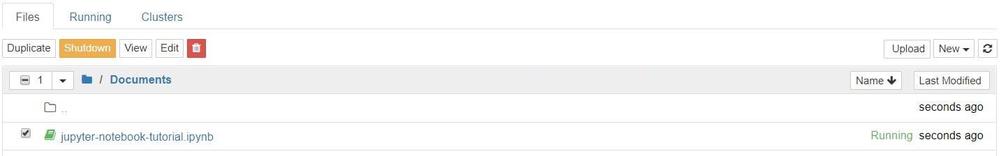
Setup
It’s common to start off with a code cell specifically for imports and setup, so that if you choose to add or change anything, you can simply edit and re-run the cell without causing any side-effects.
%matplotlib inline
import pandas as pd
import matplotlib.pyplot as plt
import seaborn as sns sns.set(style="darkgrid")
We’ll import pandas to work with our data, Matplotlib to plot charts, and Seaborn to make our charts prettier. It’s also common to import NumPy but in this case, pandas imports it for us.
That first line isn’t a Python command, but uses something called a line magic to instruct Jupyter to capture Matplotlib plots and render them in the cell output. We’ll talk a bit more about line magics later, and they’re also covered in our advanced Jupyter Notebooks tutorial.
For now, let’s go ahead and load our data.
df = pd.read_csv('fortune500.csv')It’s sensible to also do this in a single cell, in case we need to reload it at any point.
Save and Checkpoint
Now we’ve got started, it’s best practice to save regularly. Pressing Ctrl + S will save our notebook by calling the “Save and Checkpoint” command, but what is this checkpoint thing?
Every time we create a new notebook, a checkpoint file is created along with the notebook file. It is located within a hidden subdirectory of your save location called .ipynb_checkpoints and is also a .ipynb file.
By default, Jupyter will autosave your notebook every 120 seconds to this checkpoint file without altering your primary notebook file. When you “Save and Checkpoint,” both the notebook and checkpoint files are updated. Hence, the checkpoint enables you to recover your unsaved work in the event of an unexpected issue.
You can revert to the checkpoint from the menu via “File > Revert to Checkpoint.”
Investigating Our Data Set
Now we’re really rolling! Our notebook is safely saved and we’ve loaded our data set df into the most-used pandas data structure, which is called a DataFrame and basically looks like a table. What does ours look like?
df.head()| Year | Rank | Company | Revenue (in millions) | Profit (in millions) | |
|---|---|---|---|---|---|
| 0 | 1955 | 1 | General Motors | 9823.5 | 806 |
| 1 | 1955 | 2 | Exxon Mobil | 5661.4 | 584.8 |
| 2 | 1955 | 3 | U.S. Steel | 3250.4 | 195.4 |
| 3 | 1955 | 4 | General Electric | 2959.1 | 212.6 |
| 4 | 1955 | 5 | Esmark | 2510.8 | 19.1 |
df.tail()| Year | Rank | Company | Revenue (in millions) | Profit (in millions) | |
|---|---|---|---|---|---|
| 25495 | 2005 | 496 | Wm. Wrigley Jr. | 3648.6 | 493 |
| 25496 | 2005 | 497 | Peabody Energy | 3631.6 | 175.4 |
| 25497 | 2005 | 498 | Wendy’s International | 3630.4 | 57.8 |
| 25498 | 2005 | 499 | Kindred Healthcare | 3616.6 | 70.6 |
| 25499 | 2005 | 500 | Cincinnati Financial | 3614.0 | 584 |
Looking good. We have the columns we need, and each row corresponds to a single company in a single year.
Let’s just rename those columns so we can refer to them later.
df.columns = ['year', 'rank', 'company', 'revenue', 'profit']Next, we need to explore our data set. Is it complete? Did pandas read it as expected? Are any values missing?
len(df)25500Okay, that looks good — that’s 500 rows for every year from 1955 to 2005, inclusive.
Let’s check whether our data set has been imported as we would expect. A simple check is to see if the data types (or dtypes) have been correctly interpreted.
df.dtypesyear int64 rank int64 company object revenue float64 profit object dtype: objectUh oh. It looks like there’s something wrong with the profits column — we would expect it to be a float64 like the revenue column. This indicates that it probably contains some non-integer values, so let’s take a look.
non_numberic_profits = df.profit.str.contains('[^0-9.-]')
df.loc[non_numberic_profits].head()| year | rank | company | revenue | profit | |
|---|---|---|---|---|---|
| 228 | 1955 | 229 | Norton | 135.0 | N.A. |
| 290 | 1955 | 291 | Schlitz Brewing | 100.0 | N.A. |
| 294 | 1955 | 295 | Pacific Vegetable Oil | 97.9 | N.A. |
| 296 | 1955 | 297 | Liebmann Breweries | 96.0 | N.A. |
| 352 | 1955 | 353 | Minneapolis-Moline | 77.4 | N.A. |
Just as we suspected! Some of the values are strings, which have been used to indicate missing data. Are there any other values that have crept in?
set(df.profit[non_numberic_profits]){'N.A.'}That makes it easy to interpret, but what should we do? Well, that depends how many values are missing.
len(df.profit[non_numberic_profits])369It’s a small fraction of our data set, though not completely inconsequential as it is still around 1.5%.
If rows containing N.A. are, roughly, uniformly distributed over the years, the easiest solution would just be to remove them. So let’s have a quick look at the distribution.
bin_sizes, _, _ = plt.hist(df.year[non_numberic_profits], bins=range(1955, 2006))
At a glance, we can see that the most invalid values in a single year is fewer than 25, and as there are 500 data points per year, removing these values would account for less than 4% of the data for the worst years. Indeed, other than a surge around the 90s, most years have fewer than half the missing values of the peak.
For our purposes, let’s say this is acceptable and go ahead and remove these rows.
df = df.loc[~non_numberic_profits]
df.profit = df.profit.apply(pd.to_numeric)
We should check that worked.
len(df)25131df.dtypesyear int64 rank int64 company object revenue float64 profit float64 dtype: objectGreat! We have finished our data set setup.
If we were going to present your notebook as a report, we could get rid of the investigatory cells we created, which are included here as a demonstration of the flow of working with notebooks, and merge relevant cells (see the Advanced Functionality section below for more on this) to create a single data set setup cell.
This would mean that if we ever mess up our data set elsewhere, we can just rerun the setup cell to restore it.
Plotting with matplotlib
Next, we can get to addressing the question at hand by plotting the average profit by year. We might as well plot the revenue as well, so first we can define some variables and a method to reduce our code.
group_by_year = df.loc[:, ['year', 'revenue', 'profit']].groupby('year')
avgs = group_by_year.mean()
x = avgs.index
y1 = avgs.profit
def plot(x, y, ax, title, y_label):
    ax.set_title(title)
    ax.set_ylabel(y_label)
    ax.plot(x, y)
    ax.margins(x=0, y=0)
Now let’s plot!
fig, ax = plt.subplots()
plot(x, y1, ax, 'Increase in mean Fortune 500 company profits from 1955 to 2005', 'Profit (millions)')
Wow, that looks like an exponential, but it’s got some huge dips. They must correspond to the early 1990s recession and the dot-com bubble. It’s pretty interesting to see that in the data. But how come profits recovered to even higher levels post each recession?
Maybe the revenues can tell us more.
y2 = avgs.revenue
fig, ax = plt.subplots()
plot(x, y2, ax, 'Increase in mean Fortune 500 company revenues from 1955 to 2005', 'Revenue (millions)')
That adds another side to the story. Revenues were not as badly hit — that’s some great accounting work from the finance departments.
With a little help from Stack Overflow, we can superimpose these plots with +/- their standard deviations.
def plot_with_std(x, y, stds, ax, title, y_label):
    ax.fill_between(x, y - stds, y + stds, alpha=0.2)
    plot(x, y, ax, title, y_label)
fig, (ax1, ax2) = plt.subplots(ncols=2)
title = 'Increase in mean and std Fortune 500 company %s from 1955 to 2005'
stds1 = group_by_year.std().profit.values
stds2 = group_by_year.std().revenue.values
plot_with_std(x, y1.values, stds1, ax1, title % 'profits', 'Profit (millions)')
plot_with_std(x, y2.values, stds2, ax2, title % 'revenues', 'Revenue (millions)')
fig.set_size_inches(14, 4)
fig.tight_layout()
That’s staggering, the standard deviations are huge! Some Fortune 500 companies make billions while others lose billions, and the risk has increased along with rising profits over the years.
Perhaps some companies perform better than others; are the profits of the top 10% more or less volatile than the bottom 10%?
There are plenty of questions that we could look into next, and it’s easy to see how the flow of working in a notebook can match one’s own thought process. For the purposes of this tutorial, we’ll stop our analysis here, but feel free to continue digging into the data on your own!
This flow helped us to easily investigate our data set in one place without context switching between applications, and our work is immediately shareable and reproducible. If we wished to create a more concise report for a particular audience, we could quickly refactor our work by merging cells and removing intermediary code.
Sharing Your Notebooks
When people talk about sharing their notebooks, there are generally two paradigms they may be considering.
Most often, individuals share the end-result of their work, much like this article itself, which means sharing non-interactive, pre-rendered versions of their notebooks. However, it is also possible to collaborate on notebooks with the aid of version control systems such as Git or online platforms like Google Colab.
Before You Share
A shared notebook will appear exactly in the state it was in when you export or save it, including the output of any code cells. Therefore, to ensure that your notebook is share-ready, so to speak, there are a few steps you should take before sharing:
- Click “Cell > All Output > Clear”
- Click “Kernel > Restart & Run All”
- Wait for your code cells to finish executing and check ran as expected
This will ensure your notebooks don’t contain intermediary output, have a stale state, and execute in order at the time of sharing.
Exporting Your Notebooks
Jupyter has built-in support for exporting to HTML and PDF as well as several other formats, which you can find from the menu under “File > Download As.”
If you wish to share your notebooks with a small private group, this functionality may well be all you need. Indeed, as many researchers in academic institutions are given some public or internal webspace, and because you can export a notebook to an HTML file, Jupyter Notebooks can be an especially convenient way for researchers to share their results with their peers.
But if sharing exported files doesn’t cut it for you, there are also some immensely popular methods of sharing .ipynb files more directly on the web.
GitHub
With the number of public notebooks on GitHub exceeding 1.8 million by early 2018, it is surely the most popular independent platform for sharing Jupyter projects with the world. GitHub has integrated support for rendering .ipynb files directly both in repositories and gists on its website. If you aren’t already aware, GitHub is a code hosting platform for version control and collaboration for repositories created with Git. You’ll need an account to use their services, but standard accounts are free.
Once you have a GitHub account, the easiest way to share a notebook on GitHub doesn’t actually require Git at all. Since 2008, GitHub has provided its Gist service for hosting and sharing code snippets, which each get their own repository. To share a notebook using Gists:
- Sign in and navigate to gist.github.com.
- Open your
.ipynbfile in a text editor, select all and copy the JSON inside. - Paste the notebook JSON into the gist.
- Give your Gist a filename, remembering to add
.iypnbor this will not work. - Click either “Create secret gist” or “Create public gist.”
This should look something like the following:
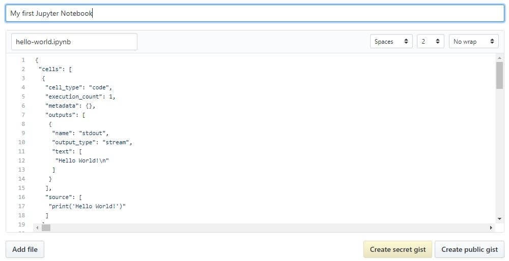
If you created a public Gist, you will now be able to share its URL with anyone, and others will be able to fork and clone your work.
Creating your own Git repository and sharing this on GitHub is beyond the scope of this tutorial, but GitHub provides plenty of guides for you to get started on your own.
An extra tip for those using git is to add an exception to your .gitignore for those hidden .ipynb_checkpoints directories Jupyter creates, so as not to commit checkpoint files unnecessarily to your repo.
Nbviewer
Having grown to render hundreds of thousands of notebooks every week by 2015, NBViewer is the most popular notebook renderer on the web. If you already have somewhere to host your Jupyter Notebooks online, be it GitHub or elsewhere, NBViewer will render your notebook and provide a shareable URL along with it. Provided as a free service as part of Project Jupyter, it is available at nbviewer.jupyter.org.
Initially developed before GitHub’s Jupyter Notebook integration, NBViewer allows anyone to enter a URL, Gist ID, or GitHub username/repo/file and it will render the notebook as a webpage. A Gist’s ID is the unique number at the end of its URL; for example, the string of characters after the last backslash in https://gist.github.com/username/50896401c23e0bf417e89cd57e89e1de. If you enter a GitHub username or username/repo, you will see a minimal file browser that lets you explore a user’s repos and their contents.
The URL NBViewer displays when displaying a notebook is a constant based on the URL of the notebook it is rendering, so you can share this with anyone and it will work as long as the original files remain online — NBViewer doesn’t cache files for very long.
If you don’t like Nbviewer, there are other similar options — here’s a thread with a few to consider from our community.
Extras: Jupyter Notebook Extensions
We’ve already covered everything you need to get rolling in Jupyter Notebooks.
What Are Extensions?
Extensions are precisely what they sound like — additional features that extend Jupyter Notebooks’s functionality. While a base Jupyter Notebook can do an awful lot, extensions offer some additional features that may help with specific workflows, or that simply improve the user experience.
For example, one extension called «Table of Contents» generates a table of contents for your notebook, to make large notebooks easier to visualize and navigate around.
Another one, called Variable Inspector, will show you the value, type, size, and shape of every variable in your notebook for easy quick reference and debugging.
Another, called ExecuteTime, lets you know when and for how long each cell ran — this can be particularly convenient if you’re trying to speed up a snippet of your code.
These are just the tip of the iceberg; there are many extensions available.
Where Can You Get Extensions?
To get the extensions, you need to install Nbextensions. You can do this using pip and the command line. If you have Anaconda, it may be better to do this through Anaconda Prompt rather than the regular command line.
Close Jupyter Notebooks, open Anaconda Prompt, and run the following command: pip install jupyter_contrib_nbextensions && jupyter contrib nbextension install.
Once you’ve done that, start up a notebook and you should seen an Nbextensions tab. Clicking this tab will show you a list of available extensions. Simply tick the boxes for the extensions you want to enable, and you’re off to the races!
Installing Extensions
Once Nbextensions itself has been installed, there’s no need for additional installation of each extension. However, if you’ve already installed Nbextensons but aren’t seeing the tab, you’re not alone. This thread on Github details some common issues and solutions.
Extras: Line Magics in Jupyter
We mentioned magic commands earlier when we used %matplotlib inline to make Matplotlib charts render right in our notebook. There are many other magics we can use, too.
How to Use Magics in Jupyter
A good first step is to open a Jupyter Notebook, type %lsmagic into a cell, and run the cell. This will output a list of the available line magics and cell magics, and it will also tell you whether «automagic» is turned on.
- Line magics operate on a single line of a code cell
- Cell magics operate on the entire code cell in which they are called
If automagic is on, you can run a magic simply by typing it on its own line in a code cell, and running the cell. If it is off, you will need to put % before line magics and %% before cell magics to use them.
Many magics require additional input (much like a function requires an argument) to tell them how to operate. We’ll look at an example in the next section, but you can see the documentation for any magic by running it with a question mark, like so:
%matplotlib?When you run the above cell in a notebook, a lengthy docstring will pop up onscreen with details about how you can use the magic.
A Few Useful Magic Commands
We cover more in the advanced Jupyter tutorial, but here are a few to get you started:
| Magic Command | What it does |
|---|---|
| %run | Runs an external script file as part of the cell being executed.
For example, if %run myscript.py appears in a code cell, myscript.py will be executed by the kernel as part of that cell. |
| %timeit | Counts loops, measures and reports how long a code cell takes to execute. |
| %writefile | Save the contents of a cell to a file.
For example, %savefile myscript.py would save the code cell as an external file called myscript.py. |
| %store | Save a variable for use in a different notebook. |
| %pwd | Print the directory path you’re currently working in. |
| %%javascript | Runs the cell as JavaScript code. |
There’s plenty more where that came from. Hop into Jupyter Notebooks and start exploring using %lsmagic!
Final Thoughts
Starting from scratch, we have come to grips with the natural workflow of Jupyter Notebooks, delved into IPython’s more advanced features, and finally learned how to share our work with friends, colleagues, and the world. And we accomplished all this from a notebook itself!
It should be clear how notebooks promote a productive working experience by reducing context switching and emulating a natural development of thoughts during a project. The power of using Jupyter Notebooks should also be evident, and we covered plenty of leads to get you started exploring more advanced features in your own projects.
If you’d like further inspiration for your own Notebooks, Jupyter has put together a gallery of interesting Jupyter Notebooks that you may find helpful and the Nbviewer homepage links to some really fancy examples of quality notebooks.
If you’d like to learn more about this topic, check out Dataquest’s interactive Python Functions and Learn Jupyter Notebook course, and our Data Analyst in Python, and Data Scientist in Python paths that will help you become job-ready in around 6 months.
More Great Jupyter Notebooks Resources
- Advanced Jupyter Notebooks Tutorial – Now that you’ve mastered the basics, become a Jupyter Notebooks pro with this advanced tutorial!
- 28 Jupyter Notebooks Tips, Tricks, and Shortcuts – Make yourself into a power user and increase your efficiency with these tips and tricks!
- Guided Project – Install and Learn Jupyter Notebooks – Give yourself a great foundation working with Jupyter Notebooks by working through this interactive guided project that’ll get you set up and teach you the ropes.