MATLAB – Обзор
MATLAB (матричная лаборатория) – это язык программирования высокого уровня четвертого поколения и интерактивная среда для численных расчетов, визуализации и программирования.
MATLAB разработан MathWorks.
Это позволяет матричные манипуляции; построение графиков функций и данных; реализация алгоритмов; создание пользовательских интерфейсов; взаимодействие с программами, написанными на других языках, включая C, C ++, Java и FORTRAN; анализировать данные; разработать алгоритмы; и создавать модели и приложения.
Он имеет множество встроенных команд и математических функций, которые помогают вам в математических вычислениях, создании графиков и выполнении численных методов.
Сила вычислительной математики MATLAB
MATLAB используется во всех аспектах вычислительной математики. Ниже приведены некоторые часто используемые математические вычисления, где он используется чаще всего:
- Работа с матрицами и массивами
- 2-D и 3-D Печать и графика
- Линейная алгебра
- Алгебраические уравнения
- Нелинейные функции
- Статистика
- Анализ данных
- Исчисление и дифференциальные уравнения
- Численные расчеты
- интеграция
- Трансформации
- Кривая Фитинг
- Различные другие специальные функции
Особенности MATLAB
Ниже приведены основные характеристики MATLAB –
-
Это язык высокого уровня для численных расчетов, визуализации и разработки приложений.
-
Он также предоставляет интерактивную среду для итеративного исследования, проектирования и решения проблем.
-
Он предоставляет обширную библиотеку математических функций для линейной алгебры, статистики, анализа Фурье, фильтрации, оптимизации, численного интегрирования и решения обыкновенных дифференциальных уравнений.
-
Он предоставляет встроенную графику для визуализации данных и инструменты для создания пользовательских графиков.
-
Интерфейс программирования MATLAB предоставляет инструменты для разработки, позволяющие повысить качество сопровождения кода и максимально повысить производительность.
-
Он предоставляет инструменты для создания приложений с пользовательскими графическими интерфейсами.
-
Он предоставляет функции для интеграции алгоритмов на основе MATLAB с внешними приложениями и языками, такими как C, Java, .NET и Microsoft Excel.
Это язык высокого уровня для численных расчетов, визуализации и разработки приложений.
Он также предоставляет интерактивную среду для итеративного исследования, проектирования и решения проблем.
Он предоставляет обширную библиотеку математических функций для линейной алгебры, статистики, анализа Фурье, фильтрации, оптимизации, численного интегрирования и решения обыкновенных дифференциальных уравнений.
Он предоставляет встроенную графику для визуализации данных и инструменты для создания пользовательских графиков.
Интерфейс программирования MATLAB предоставляет инструменты для разработки, позволяющие повысить качество сопровождения кода и максимально повысить производительность.
Он предоставляет инструменты для создания приложений с пользовательскими графическими интерфейсами.
Он предоставляет функции для интеграции алгоритмов на основе MATLAB с внешними приложениями и языками, такими как C, Java, .NET и Microsoft Excel.
Использование MATLAB
MATLAB широко используется в качестве вычислительного инструмента в науке и технике, охватывающего области физики, химии, математики и всех технических потоков. Он используется в различных областях, в том числе –
- Обработка сигналов и связь
- Обработка изображений и видео
- Системы управления
- Тест и Измерение
- Вычислительные финансы
- Вычислительная биология
MATLAB – Настройка среды
Настройка локальной среды
Настройка среды MATLAB производится в несколько кликов. Установщик можно скачать здесь .
MathWorks предоставляет лицензионный продукт, пробную версию, а также студенческую версию. Вам необходимо зайти на сайт и немного подождать их одобрения.
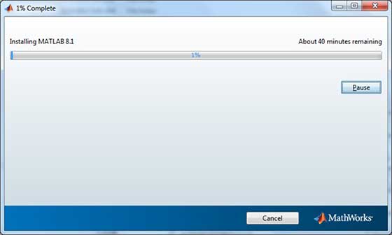
После загрузки установщика программное обеспечение можно установить с помощью нескольких кликов.

Понимание среды MATLAB
Среду разработки MATLAB можно запустить из иконки, созданной на рабочем столе. Основное рабочее окно в MATLAB называется рабочим столом. Когда MATLAB запущен, рабочий стол отображается в макете по умолчанию –

Рабочий стол имеет следующие панели –
-
Текущая папка – эта панель позволяет получить доступ к папкам и файлам проекта.
-
Окно команд – это основная область, где команды можно вводить в командной строке. На это указывает командная строка (>>).
-
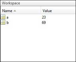
Рабочая область – Рабочая область показывает все переменные, созданные и / или импортированные из файлов.
-
История команд – эта панель показывает или возвращает команды, которые вводятся в командной строке.


Текущая папка – эта панель позволяет получить доступ к папкам и файлам проекта.
Окно команд – это основная область, где команды можно вводить в командной строке. На это указывает командная строка (>>).
Рабочая область – Рабочая область показывает все переменные, созданные и / или импортированные из файлов.
История команд – эта панель показывает или возвращает команды, которые вводятся в командной строке.
Настройка GNU Octave
Если вы хотите использовать Octave на своем компьютере (Linux, BSD, OS X или Windows), пожалуйста, скачайте последнюю версию с Download GNU Octave . Вы можете проверить данные инструкции по установке для вашей машины.
MATLAB – базовый синтаксис
Среда MATLAB ведет себя как сверхсложный калькулятор. Вы можете вводить команды в командной строке >>.
MATLAB – это интерпретируемая среда. Другими словами, вы даете команду, а MATLAB выполняет ее сразу.
Руки на практике
Введите правильное выражение, например,
Live Demo
5 + 5
И нажмите ENTER
Когда вы нажимаете кнопку «Выполнить» или нажимаете Ctrl + E, MATLAB выполняет его немедленно, и возвращается результат –
ans = 10
Давайте рассмотрим еще несколько примеров –
Live Demo
3 ^ 2 % 3 raised to the power of 2
Когда вы нажимаете кнопку «Выполнить» или нажимаете Ctrl + E, MATLAB выполняет его немедленно, и возвращается результат –
ans = 9
Другой пример,
Live Demo
sin(pi /2) % sine of angle 90 o
Когда вы нажимаете кнопку «Выполнить» или нажимаете Ctrl + E, MATLAB выполняет его немедленно, и возвращается результат –
ans = 1
Другой пример,
Live Demo
7/0 % Divide by zero
Когда вы нажимаете кнопку «Выполнить» или нажимаете Ctrl + E, MATLAB выполняет его немедленно, и возвращается результат –
ans = Inf
warning: division by zero
Другой пример,
Live Demo
732 * 20.3
Когда вы нажимаете кнопку «Выполнить» или нажимаете Ctrl + E, MATLAB выполняет его немедленно, и возвращается результат –
ans = 1.4860e+04
MATLAB предоставляет некоторые специальные выражения для некоторых математических символов, таких как pi для π, Inf для ∞, i (и j) для √-1 и т. Д. Nan означает «не число».
Использование точки с запятой (;) в MATLAB
Точка с запятой (;) указывает на конец оператора. Однако, если вы хотите подавить и скрыть вывод MATLAB для выражения, добавьте точку с запятой после выражения.
Например,
Live Demo
x = 3;
y = x + 5
Когда вы нажимаете кнопку «Выполнить» или нажимаете Ctrl + E, MATLAB выполняет его немедленно, и возвращается результат –
y = 8
Добавление комментариев
Символ процента (%) используется для обозначения строки комментария. Например,
x = 9 % assign the value 9 to x
Вы также можете написать блок комментариев, используя операторы комментариев к блоку% {и%}.
Редактор MATLAB включает в себя инструменты и элементы контекстного меню, которые помогут вам добавлять, удалять или изменять формат комментариев.
Обычно используемые операторы и специальные символы
MATLAB поддерживает следующие часто используемые операторы и специальные символы –
| оператор | Цель |
|---|---|
| + | Плюс; оператор сложения. |
| – | Минус; оператор вычитания. |
| * | Скалярный и матричный оператор умножения. |
| . * | Оператор умножения массива. |
| ^ | Скалярный и матричный оператор возведения в степень. |
| . ^ | Оператор возведения в степень массива. |
| Оператор левого деления. | |
| / | Оператор правого деления. |
| . | Массив левого делителя. |
| ./ | Массив оператора правого деления. |
| : | Двоеточие; генерирует регулярно расположенные элементы и представляет всю строку или столбец. |
| () | Скобки; заключает в себе аргументы функций и индексы массивов; переопределяет приоритет |
| [] | Скобки; элементы массива вложений. |
| , | Десятичная точка. |
| … | Многоточие; оператор продолжения строки |
| , | Comma; разделяет операторы и элементы подряд |
| ; | Точка с запятой; разделяет столбцы и подавляет отображение. |
| % | Знак процента; обозначает комментарий и задает форматирование. |
| _ | Цитировать знак и транспонировать оператора. |
| ._ | Несопряженный оператор транспонирования. |
| знак равно | Оператор присваивания. |
Специальные переменные и константы
MATLAB поддерживает следующие специальные переменные и константы –
| название | Имея в виду |
|---|---|
| анс | Самый последний ответ. |
| прибыль на акцию | Точность точности с плавающей точкой. |
| I, J | Мнимая единица √-1. |
| Inf | Бесконечность. |
| NaN | Неопределенный числовой результат (не число). |
| число Пи | Число π |
Именование переменных
Имена переменных состоят из буквы, за которой следует любое количество букв, цифр или подчеркивания.
MATLAB чувствителен к регистру .
Имена переменных могут быть любой длины, однако MATLAB использует только первые N символов, где N задается функцией namelengthmax .
Сохранение вашей работы
Команда save используется для сохранения всех переменных в рабочей области в виде файла с расширением .mat в текущем каталоге.
Например,
save myfile
Вы можете перезагрузить файл в любое время позже, используя команду загрузки .
load myfile
MATLAB – Переменные
В среде MATLAB каждая переменная является массивом или матрицей.
Вы можете назначить переменные простым способом. Например,
Live Demo
x = 3 % defining x and initializing it with a value
MATLAB выполнит приведенный выше оператор и вернет следующий результат –
x = 3
Он создает матрицу 1 на 1 с именем x и сохраняет значение 3 в своем элементе. Давайте посмотрим на другой пример,
Live Demo
x = sqrt(16) % defining x and initializing it with an expression
MATLAB выполнит приведенный выше оператор и вернет следующий результат –
x = 4
Пожалуйста, обратите внимание, что –
-
Как только переменная введена в систему, вы можете обратиться к ней позже.
-
Переменные должны иметь значения, прежде чем они будут использованы.
-
Когда выражение возвращает результат, который не присвоен какой-либо переменной, система назначает его переменной с именем ans, которая может быть использована позже.
Как только переменная введена в систему, вы можете обратиться к ней позже.
Переменные должны иметь значения, прежде чем они будут использованы.
Когда выражение возвращает результат, который не присвоен какой-либо переменной, система назначает его переменной с именем ans, которая может быть использована позже.
Например,
Live Demo
sqrt(78)
MATLAB выполнит приведенный выше оператор и вернет следующий результат –
ans = 8.8318
Вы можете использовать эту переменную ANS –
Live Demo
sqrt(78);
9876/ans
MATLAB выполнит приведенный выше оператор и вернет следующий результат –
ans = 1118.2
Давайте посмотрим на другой пример –
Live Demo
x = 7 * 8;
y = x * 7.89
MATLAB выполнит приведенный выше оператор и вернет следующий результат –
y = 441.84
Несколько назначений
Вы можете иметь несколько назначений на одной строке. Например,
Live Demo
a = 2; b = 7; c = a * b
MATLAB выполнит приведенный выше оператор и вернет следующий результат –
c = 14
Я забыл переменные!
Команда who отображает все имена переменных, которые вы использовали.
who
MATLAB выполнит приведенный выше оператор и вернет следующий результат –
Your variables are:
a    ans  b    c
Команда whos показывает немного больше о переменных –
- Переменные в настоящее время в памяти
- Тип каждой переменной
- Память, выделенная для каждой переменной
- Являются ли они сложными переменными или нет
whos
MATLAB выполнит приведенный выше оператор и вернет следующий результат –
Attr Name        Size        Bytes      Class
==== ====        ====        ====       =====
   a             1x1           8        double
   ans           1x70         757        cell
   b             1x1           8        double
   c             1x1           8        double

Total is 73 elements using 781 bytes
Команда очистки удаляет все (или указанные) переменные из памяти.
clear x     % it will delete x, won't display anything
clear       % it will delete all variables in the workspace
            %  peacefully and unobtrusively
Длинные Задания
Длинные назначения могут быть расширены до другой строки с помощью эллипсов (…). Например,
Live Demo
initial_velocity = 0;
acceleration = 9.8;
time = 20;
final_velocity = initial_velocity + acceleration * time
MATLAB выполнит приведенный выше оператор и вернет следующий результат –
final_velocity = 196
Формат Команда
По умолчанию MATLAB отображает числа с четырьмя знаками после запятой. Это известно как короткий формат .
Однако, если вы хотите большей точности, вам нужно использовать команду форматирования .
Команда format long отображает 16 цифр после десятичной дроби.
Например –
Live Demo
format long
x = 7 + 10/3 + 5 ^ 1.2
MATLAB выполнит приведенный выше оператор и вернет следующий результат:
x = 17.2319816406394
Другой пример,
Live Demo
format short
x = 7 + 10/3 + 5 ^ 1.2
MATLAB выполнит приведенный выше оператор и вернет следующий результат –
x = 17.232
Команда формата банка округляет числа до двух десятичных знаков. Например,
Live Demo
format bank
daily_wage = 177.45;
weekly_wage = daily_wage * 6
MATLAB выполнит приведенный выше оператор и вернет следующий результат –
weekly_wage = 1064.70
MATLAB отображает большие числа с использованием экспоненциальной записи.
Команда format short e позволяет отображать в экспоненциальной форме с четырьмя десятичными знаками плюс показатель степени.
Например,
Live Demo
format short e
4.678 * 4.9
MATLAB выполнит приведенный выше оператор и вернет следующий результат –
ans = 2.2922e+01
Команда format long e позволяет отображать в экспоненциальной форме с четырьмя десятичными знаками плюс показатель степени. Например,
Live Demo
format long e
x = pi
MATLAB выполнит приведенный выше оператор и вернет следующий результат –
x = 3.141592653589793e+00
Команда format rat дает наиболее близкое рациональное выражение, полученное в результате вычисления. Например,
Live Demo
format rat
4.678 * 4.9
MATLAB выполнит приведенный выше оператор и вернет следующий результат –
ans = 34177/1491
Создание векторов
Вектор – это одномерный массив чисел. MATLAB позволяет создавать два типа векторов –
- Векторы строк
- Векторы столбцов
Векторы строк создаются путем заключения набора элементов в квадратных скобках с использованием пробела или запятой для разделения элементов.
Например,
Live Demo
r = [7 8 9 10 11]
MATLAB выполнит приведенный выше оператор и вернет следующий результат –
r =

   7    8    9   10   11
Другой пример,
Live Demo
r = [7 8 9 10 11];
t = [2, 3, 4, 5, 6];
res = r + t
MATLAB выполнит приведенный выше оператор и вернет следующий результат –
res =

         9         11         13         15         17
Векторы столбцов создаются заключением набора элементов в квадратные скобки с использованием точки с запятой (;) для разделения элементов.
Live Demo
c = [7; 8; 9; 10; 11]
MATLAB выполнит приведенный выше оператор и вернет следующий результат –
c =
       7
       8
       9
      10
      11
Создание Матрицы
Матрица – это двумерный массив чисел.
В MATLAB матрица создается путем ввода каждой строки в виде последовательности элементов, разделенных пробелами или запятыми, и конец строки обозначается точкой с запятой. Например, давайте создадим матрицу 3 на 3 как –
Live Demo
m = [1 2 3; 4 5 6; 7 8 9]
MATLAB выполнит приведенный выше оператор и вернет следующий результат –
m =
       1              2              3
       4              5              6
       7              8              9
MATLAB – Команды
MATLAB – интерактивная программа для численных расчетов и визуализации данных. Вы можете ввести команду, набрав ее в командной строке MATLAB ‘>>’ в окне команд .
В этом разделе мы предоставим списки часто используемых общих команд MATLAB.
Команды для управления сеансом
MATLAB предоставляет различные команды для управления сеансом. В следующей таблице приведены все такие команды:
| команда | Цель |
|---|---|
| CLC | Очищает командное окно. |
| Чисто | Удаляет переменные из памяти. |
| существовать | Проверяет наличие файла или переменной. |
| Глобальный | Объявляет переменные глобальными. |
| Помогите | Ищет справочную тему. |
| Ищу | Поиск записей справки по ключевому слову. |
| уволиться | Останавливается MATLAB. |
| кто | Перечисляет текущие переменные. |
| Whos | Перечисляет текущие переменные (длинный дисплей). |
Команды для работы с системой
MATLAB предоставляет различные полезные команды для работы с системой, такие как сохранение текущей работы в рабочей области в виде файла и загрузка файла позже.
Он также предоставляет различные команды для других действий, связанных с системой, таких как отображение даты, отображение списка файлов в каталоге, отображение текущего каталога и т. Д.
В следующей таблице приведены некоторые часто используемые системные команды:
| команда | Цель |
|---|---|
| CD | Изменяет текущий каталог. |
| Дата | Отображает текущую дату. |
| удалять | Удаляет файл. |
| дневник | Включает / выключает запись в дневниковый файл. |
| реж | Перечисляет все файлы в текущем каталоге. |
| нагрузка | Загружает переменные рабочей области из файла. |
| дорожка | Отображает путь поиска. |
| PWD | Отображает текущий каталог. |
| спасти | Сохраняет переменные рабочей области в файл. |
| тип | Отображает содержимое файла. |
| какие | Перечисляет все файлы MATLAB в текущем каталоге. |
| wklread | Читает файл электронной таблицы .wk1. |
Команды ввода и вывода
MATLAB предоставляет следующие команды ввода и вывода –
| команда | Цель |
|---|---|
| Индик.точки | Отображает содержимое массива или строки. |
| fscanf | Чтение отформатированных данных из файла. |
| формат | Управляет форматом отображения экрана. |
| fprintf | Выполняет отформатированные записи на экран или в файл. |
| вход | Отображает подсказки и ждет ввода. |
| ; | Подавляет трафаретную печать. |
Команды fscanf и fprintf ведут себя как функции C scanf и printf. Они поддерживают следующие коды формата –
| Код формата | Цель |
|---|---|
| % s | Форматировать как строку. |
| % d | Форматировать как целое число. |
| % е | Формат как значение с плавающей запятой. |
| % е | Формат как значение с плавающей запятой в научной нотации. |
| %г | Формат в наиболее компактной форме:% f или% e. |
| п | Вставьте новую строку в выходную строку. |
| т | Вставьте вкладку в выходной строке. |
Функция форматирования имеет следующие формы, используемые для числового отображения:
| Функция формата | Отображать до |
|---|---|
| формат короткий | Четыре десятичных знака (по умолчанию). |
| форматировать долго | 16 десятичных цифр. |
| формат короткой электронной | Пять цифр плюс показатель степени. |
| формат длинная электронная | 16 цифр плюс показатели. |
| формат банка | Две десятичные цифры. |
| формат + | Положительный, отрицательный или ноль. |
| формат крыса | Рациональное приближение. |
| формат компактный | Подавляет некоторые переводы строки. |
| свободный формат | Сбрасывает в менее компактный режим отображения. |
Векторные, матричные и матричные команды
В следующей таблице показаны различные команды, используемые для работы с массивами, матрицами и векторами.
| команда | Цель |
|---|---|
| кошка | Объединяет массивы. |
| находить | Находит индексы ненулевых элементов. |
| длина | Вычисляет количество элементов. |
| LINSPACE | Создает равномерно расположенный вектор. |
| logspace | Создает логарифмически разнесенный вектор. |
| Максимум | Возвращает самый большой элемент. |
| мин | Возвращает наименьший элемент. |
| тычок | Продукт каждого столбца. |
| перекроить | Изменяет размер. |
| размер | Вычисляет размер массива. |
| Сортировать | Сортирует каждый столбец. |
| сумма | Суммирует каждый столбец. |
| глаз | Создает идентичную матрицу. |
| те, | Создает массив из них. |
| нули | Создает массив нулей. |
| пересекать | Вычисляет матричные перекрестные произведения. |
| точка | Вычисляет матричные точечные произведения. |
| йе | Вычисляет определитель массива. |
| фактура | Вычисляет обратную матрицу. |
| pinv | Вычисляет псевдообратную матрицу. |
| ранг | Вычисляет ранг матрицы. |
| RREF | Вычисляет приведенную форму ряда эшелонов. |
| клетка | Создает массив ячеек. |
| celldisp | Отображает массив ячеек. |
| cellplot | Отображает графическое представление массива ячеек. |
| num2cell | Преобразует числовой массив в массив ячеек. |
| по рукам | Соответствует спискам ввода и вывода. |
| iscell | Определяет массив ячеек. |
Команды построения
MATLAB предоставляет многочисленные команды для построения графиков. В следующей таблице приведены некоторые из наиболее часто используемых команд для построения графиков:
| команда | Цель |
|---|---|
| ось | Устанавливает пределы оси. |
| fplot | Интеллектуальное построение функций. |
| сетка | Отображает линии сетки. |
| сюжет | Создает график xy. |
| Распечатать | Печать графика или сохранение графика в файл. |
| заглавие | Размещает текст в верхней части сюжета. |
| xlabel | Добавляет текстовую метку к оси X. |
| ylabel | Добавляет текстовую метку к оси Y. |
| оси | Создает объекты осей. |
| близко | Закрывает текущий сюжет. |
| закрыть все | Закрывает все участки. |
| фигура | Открывает новое окно фигуры. |
| gtext | Включает размещение метки с помощью мыши. |
| держать | Замораживает текущий сюжет. |
| легенда | Размещение легенды мышью. |
| обновление | Перерисовывает текущее окно рисунка. |
| задавать | Определяет свойства объектов, таких как оси. |
| подзаговор | Создает участки в подокнах. |
| текст | Размещает строку на рисунке. |
| бар | Создает гистограмму. |
| loglog | Создает лог-лог сюжет. |
| полярный | Создает полярный сюжет. |
| semilogx | Создает полулогичный сюжет. (логарифмическая абсцисса). |
| semilogy | Создает полулогичный сюжет. (логарифмическая ордината). |
| лестница | Создает лестничный участок. |
| стебель | Создает стволовый сюжет. |
MATLAB – M-Files
До сих пор мы использовали среду MATLAB в качестве калькулятора. Тем не менее, MATLAB также является мощным языком программирования, а также интерактивной вычислительной средой.
В предыдущих главах вы узнали, как вводить команды из командной строки MATLAB. MATLAB также позволяет записывать серии команд в файл и исполнять файл как единое целое, например, писать функцию и вызывать ее.
М-файлы
MATLAB позволяет писать два вида программных файлов –
-
Скрипты – файлы скриптов – это программные файлы с расширением .m . В этих файлах вы пишете серию команд, которые вы хотите выполнить вместе. Скрипты не принимают входные данные и не возвращают никаких выходных данных. Они оперируют данными в рабочей области.
-
Функции – файлы функций также являются программными файлами с расширением .m . Функции могут принимать входные и выходные данные. Внутренние переменные являются локальными для функции.
Скрипты – файлы скриптов – это программные файлы с расширением .m . В этих файлах вы пишете серию команд, которые вы хотите выполнить вместе. Скрипты не принимают входные данные и не возвращают никаких выходных данных. Они оперируют данными в рабочей области.
Функции – файлы функций также являются программными файлами с расширением .m . Функции могут принимать входные и выходные данные. Внутренние переменные являются локальными для функции.
Вы можете использовать редактор MATLAB или любой другой текстовый редактор для создания ваших .m файлов. В этом разделе мы обсудим файлы сценариев. Файл сценария содержит несколько последовательных строк команд MATLAB и вызовов функций. Вы можете запустить скрипт, набрав его имя в командной строке.
Создание и запуск файла скрипта
Для создания файлов скриптов вам необходимо использовать текстовый редактор. Вы можете открыть редактор MATLAB двумя способами:
- Использование командной строки
- Использование IDE
Если вы используете командную строку, введите edit в командной строке. Это откроет редактор. Вы можете напрямую ввести edit и затем имя файла (с расширением .m)
edit
Or
edit <filename>
Приведенная выше команда создаст файл в директории MATLAB по умолчанию. Если вы хотите сохранить все программные файлы в определенной папке, вам придется указать полный путь.
Давайте создадим папку с именем progs. Введите следующие команды в командной строке (>>) –
mkdir progs    % create directory progs under default directory
chdir progs    % changing the current directory to progs
edit  prog1.m  % creating an m file named prog1.m
Если вы создаете файл в первый раз, MATLAB предложит вам подтвердить его. Нажмите Да.
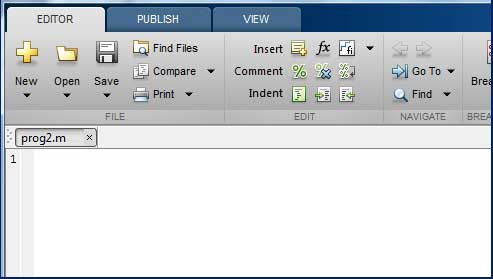
В качестве альтернативы, если вы используете IDE, выберите NEW -> Script. Это также открывает редактор и создает файл с именем Untitled. Вы можете назвать и сохранить файл после ввода кода.
Введите следующий код в редакторе –
Live Demo
NoOfStudents = 6000;
TeachingStaff = 150;
NonTeachingStaff = 20;
Total = NoOfStudents + TeachingStaff ...
   + NonTeachingStaff;
disp(Total);
После создания и сохранения файла вы можете запустить его двумя способами:
-
Нажав кнопку « Выполнить» в окне редактора или
-
Просто введите имя файла (без расширения) в командной строке: >> prog1
Нажав кнопку « Выполнить» в окне редактора или
Просто введите имя файла (без расширения) в командной строке: >> prog1
В командной строке отображается результат –
6170
пример
Создайте файл сценария и введите следующий код –
Live Demo
a = 5; b = 7;
c = a + b
d = c + sin(b)
e = 5 * d
f = exp(-d)
Когда приведенный выше код компилируется и выполняется, он дает следующий результат –
c =  12
d =  12.657
e =  63.285
f =    3.1852e-06
MATLAB – Типы данных
MATLAB не требует никакого объявления типа или операторов измерения. Всякий раз, когда MATLAB встречает новое имя переменной, он создает переменную и выделяет соответствующее пространство памяти.
Если переменная уже существует, то MATLAB заменяет исходный контент новым контентом и выделяет новое место для хранения, где это необходимо.
Например,
Total = 42
Вышеприведенный оператор создает матрицу 1 на 1 с именем «Total» и сохраняет в ней значение 42.
Типы данных, доступные в MATLAB
MATLAB предоставляет 15 основных типов данных. Каждый тип данных хранит данные в форме матрицы или массива. Размер этой матрицы или массива составляет минимум 0 на 0, и это может увеличиться до матрицы или массива любого размера.
В следующей таблице приведены наиболее часто используемые типы данных в MATLAB.
| Sr.No. | Тип данных и описание |
|---|---|
| 1 |
int8 8-разрядное целое число со знаком |
| 2 |
uint8 8-битное целое число без знака |
| 3 |
int16 16-разрядное целое число со знаком |
| 4 |
uint16 16-разрядное целое число без знака |
| 5 |
int32 32-разрядное целое число со знаком |
| 6 |
uint32 32-разрядное целое число без знака |
| 7 |
int64 64-разрядное целое число со знаком |
| 8 |
uint64 64-разрядное целое число без знака |
| 9 |
не замужем числовые данные одинарной точности |
| 10 |
двойной числовые данные двойной точности |
| 11 |
логический логические значения 1 или 0, представляют истину и ложь соответственно |
| 12 |
голец символьные данные (строки хранятся как вектор символов) |
| 13 |
массив ячеек массив индексированных ячеек, каждая из которых может хранить массив другого измерения и типа данных |
| 14 |
состав C-подобные структуры, каждая структура имеет именованные поля, способные хранить массив другого измерения и типа данных |
| 15 |
ручка функции указатель на функцию |
| 16 |
пользовательские классы объекты, созданные из определенного пользователем класса |
| 17 |
Java-классы объекты, построенные из класса Java |
int8
8-разрядное целое число со знаком
uint8
8-битное целое число без знака
int16
16-разрядное целое число со знаком
uint16
16-разрядное целое число без знака
int32
32-разрядное целое число со знаком
uint32
32-разрядное целое число без знака
int64
64-разрядное целое число со знаком
uint64
64-разрядное целое число без знака
не замужем
числовые данные одинарной точности
двойной
числовые данные двойной точности
логический
логические значения 1 или 0, представляют истину и ложь соответственно
голец
символьные данные (строки хранятся как вектор символов)
массив ячеек
массив индексированных ячеек, каждая из которых может хранить массив другого измерения и типа данных
состав
C-подобные структуры, каждая структура имеет именованные поля, способные хранить массив другого измерения и типа данных
ручка функции
указатель на функцию
пользовательские классы
объекты, созданные из определенного пользователем класса
Java-классы
объекты, построенные из класса Java
пример
Создайте файл сценария со следующим кодом –
Live Demo
str = 'Hello World!'
n = 2345
d = double(n)
un = uint32(789.50)
rn = 5678.92347
c = int32(rn)
Когда приведенный выше код компилируется и выполняется, он дает следующий результат –
str = Hello World!
n =  2345
d =  2345
un = 790
rn = 5678.9
c =  5679
Преобразование типов данных
MATLAB предоставляет различные функции для преобразования значения из одного типа данных в другой. В следующей таблице приведены функции преобразования типов данных –
| функция | Цель |
|---|---|
| голец | Преобразовать в массив символов (строку) |
| int2str | Преобразовать целочисленные данные в строку |
| mat2str | Преобразовать матрицу в строку |
| num2str | Преобразовать число в строку |
| str2double | Преобразовать строку в значение двойной точности |
| str2num | Преобразовать строку в число |
| native2unicode | Преобразуйте числовые байты в символы Юникода |
| unicode2native | Преобразование символов Юникода в числовые байты |
| base2dec | Преобразовать базовую N числовую строку в десятичное число |
| BIN2DEC | Преобразовать строку двоичного числа в десятичное число |
| dec2base | Преобразовать десятичное число в базовое число N в строке |
| DEC2BIN | Преобразовать десятичное число в двоичное число в строке |
| DEC2HEX | Преобразовать десятичное число в шестнадцатеричное число в строке |
| HEX2DEC | Преобразовать строку шестнадцатеричного числа в десятичное число |
| hex2num | Преобразовать строку шестнадцатеричного числа в число с двойной точностью |
| num2hex | Преобразование одинарных и двойных символов в шестнадцатеричные строки IEEE |
| cell2mat | Преобразовать массив ячеек в числовой массив |
| cell2struct | Преобразовать массив ячеек в массив структур |
| cellstr | Создать массив строк из массива символов |
| mat2cell | Конвертировать массив в массив ячеек с потенциально разными размерами ячеек |
| num2cell | Преобразовать массив в массив ячеек с ячейками одинакового размера |
| struct2cell | Преобразовать структуру в массив ячеек |
Определение типов данных
MATLAB предоставляет различные функции для определения типа данных переменной.
В следующей таблице приведены функции для определения типа данных переменной –
| функция | Цель |
|---|---|
| является | Определить состояние |
| это | Определите, является ли ввод объектом указанного класса |
| iscell | Определите, является ли ввод массивом ячеек |
| iscellstr | Определите, является ли ввод массивом строк |
| ischar | Определить, является ли элемент массивом символов |
| isfield | Определите, является ли входное поле структурным массивом |
| isfloat | Определите, является ли ввод массивом с плавающей точкой |
| ishghandle | Истинно для дескрипторов объектов Handle Graphics |
| isinteger | Определите, является ли ввод целочисленным массивом |
| isjava | Определите, является ли ввод Java-объектом |
| ISLOGICAL | Определите, является ли ввод логическим массивом |
| IsNumeric | Определите, является ли ввод числовым массивом |
| IsObject | Определите, является ли ввод объектом MATLAB |
| реально | Проверьте, является ли входной массив реальным |
| isscalar | Определите, является ли вход скалярным |
| isstr | Определите, является ли ввод символьным массивом |
| isstruct | Определите, является ли ввод структурным массивом |
| isvector | Определите, является ли входной вектор |
| учебный класс | Определить класс объекта |
| validateattributes | Проверьте правильность массива |
| Whos | Перечислите переменные в рабочей области, с размерами и типами |
пример
Создайте файл сценария со следующим кодом –
Live Demo
x = 3
isinteger(x)
isfloat(x)
isvector(x)
isscalar(x)
isnumeric(x)

x = 23.54
isinteger(x)
isfloat(x)
isvector(x)
isscalar(x)
isnumeric(x)

x = [1 2 3]
isinteger(x)
isfloat(x)
isvector(x)
isscalar(x)

x = 'Hello'
isinteger(x)
isfloat(x)
isvector(x)
isscalar(x)
isnumeric(x)
Когда вы запускаете файл, он дает следующий результат –
x = 3
ans = 0
ans = 1
ans = 1
ans = 1
ans = 1
x = 23.540
ans = 0
ans = 1
ans = 1
ans = 1
ans = 1
x =

          1          2          3

ans = 0
ans = 1
ans = 1
ans = 0
x = Hello
ans = 0
ans = 0
ans = 1
ans = 0
ans = 0
MATLAB – Операторы
Оператор – это символ, который указывает компилятору выполнять определенные математические или логические манипуляции. MATLAB предназначен для работы преимущественно с целыми матрицами и массивами. Следовательно, операторы в MATLAB работают как со скалярными, так и нескалярными данными. MATLAB допускает следующие виды элементарных операций –
- Арифметические Операторы
- Операторы отношений
- Логические Операторы
- Побитовые операции
- Операции над множествами
Арифметические Операторы
MATLAB допускает два различных типа арифметических операций –
- Матричные арифметические операции
- Массив арифметических операций
Матричные арифметические операции аналогичны определенным в линейной алгебре. Операции с массивами выполняются поэлементно, как в одномерном, так и в многомерном массиве.
Матричные операторы и операторы массива дифференцируются символом точки (.). Однако, поскольку операция сложения и вычитания одинакова для матриц и массивов, оператор одинаков для обоих случаев. Следующая таблица дает краткое описание операторов –
Показать примеры
| Sr.No. | Оператор и описание |
|---|---|
| 1 |
+ Дополнение или унарный плюс. A + B добавляет значения, хранящиеся в переменных A и B. A и B должны иметь одинаковый размер, если только один не является скаляром. Скаляр можно добавить в матрицу любого размера. |
| 2 |
– Вычитание или унарный минус. AB вычитает значение B из A. A и B должны иметь одинаковый размер, если только он не является скаляром. Скаляр можно вычесть из матрицы любого размера. |
| 3 |
* Матричное умножение. C = A * B – линейное алгебраическое произведение матриц A и B. Точнее,
Для нескалярных A и B число столбцов в A должно быть равно количеству строк в B. Скаляр может умножить матрицу любого размера. |
| 4 |
. * Умножение массивов. A. * B – это поэлементное произведение массивов A и B. A и B должны иметь одинаковый размер, если только один из них не является скаляром. |
| 5 |
/ Косая черта или матрица правого деления. B / A примерно такой же, как B * inv (A). Точнее, B / A = (A ‘ B’) ‘. |
| 6 |
./ Массив правого деления. A./B – матрица с элементами A (i, j) / B (i, j). A и B должны иметь одинаковый размер, если только один из них не является скаляром. |
| 7 |
Обратная косая черта или матрица левого деления. Если A – квадратная матрица, A B – примерно то же самое, что inv (A) * B, за исключением того, что она вычисляется другим способом. Если A является матрицей n-на-n и B является вектором столбцов с n компонентами, или матрицей с несколькими такими столбцами, то X = A B является решением уравнения AX = B. Предупреждающее сообщение отображается, если А плохо масштабировано или почти единственное число. |
| 8 |
. Массив покинул деление. A. B – матрица с элементами B (i, j) / A (i, j). A и B должны иметь одинаковый размер, если только один из них не является скаляром. |
| 9 |
^ Матрица власти. X ^ p есть X в степени p, если p скаляр. Если p является целым числом, мощность вычисляется путем повторного возведения в квадрат. Если целое число отрицательно, X инвертируется первым. Для других значений p в расчет включаются собственные значения и собственные векторы, например, если [V, D] = eig (X), то X ^ p = V * D. ^ p / V. |
| 10 |
. ^ Массив власти. A. ^ B – это матрица с элементами A (i, j) степени B (i, j). A и B должны иметь одинаковый размер, если только один из них не является скаляром. |
| 11 |
‘ Матрица транспонировать. A ‘- линейная алгебраическая транспонирование A. Для комплексных матриц это комплексная сопряженная транспонирование. |
| 12 |
«. Массив транспонировать. A.» это транспонирование массива A. Для сложных матриц это не связано с сопряжением. |

+
Дополнение или унарный плюс. A + B добавляет значения, хранящиеся в переменных A и B. A и B должны иметь одинаковый размер, если только один не является скаляром. Скаляр можно добавить в матрицу любого размера.
–
Вычитание или унарный минус. AB вычитает значение B из A. A и B должны иметь одинаковый размер, если только он не является скаляром. Скаляр можно вычесть из матрицы любого размера.
*
Матричное умножение. C = A * B – линейное алгебраическое произведение матриц A и B. Точнее,
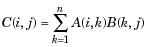
Для нескалярных A и B число столбцов в A должно быть равно количеству строк в B. Скаляр может умножить матрицу любого размера.
. *
Умножение массивов. A. * B – это поэлементное произведение массивов A и B. A и B должны иметь одинаковый размер, если только один из них не является скаляром.
/
Косая черта или матрица правого деления. B / A примерно такой же, как B * inv (A). Точнее, B / A = (A ‘ B’) ‘.
./
Массив правого деления. A./B – матрица с элементами A (i, j) / B (i, j). A и B должны иметь одинаковый размер, если только один из них не является скаляром.
Обратная косая черта или матрица левого деления. Если A – квадратная матрица, A B – примерно то же самое, что inv (A) * B, за исключением того, что она вычисляется другим способом. Если A является матрицей n-на-n и B является вектором столбцов с n компонентами, или матрицей с несколькими такими столбцами, то X = A B является решением уравнения AX = B. Предупреждающее сообщение отображается, если А плохо масштабировано или почти единственное число.
.
Массив покинул деление. A. B – матрица с элементами B (i, j) / A (i, j). A и B должны иметь одинаковый размер, если только один из них не является скаляром.
^
Матрица власти. X ^ p есть X в степени p, если p скаляр. Если p является целым числом, мощность вычисляется путем повторного возведения в квадрат. Если целое число отрицательно, X инвертируется первым. Для других значений p в расчет включаются собственные значения и собственные векторы, например, если [V, D] = eig (X), то X ^ p = V * D. ^ p / V.
. ^
Массив власти. A. ^ B – это матрица с элементами A (i, j) степени B (i, j). A и B должны иметь одинаковый размер, если только один из них не является скаляром.
‘
Матрица транспонировать. A ‘- линейная алгебраическая транспонирование A. Для комплексных матриц это комплексная сопряженная транспонирование.
«.
Массив транспонировать. A.» это транспонирование массива A. Для сложных матриц это не связано с сопряжением.
Операторы отношений
Реляционные операторы также могут работать как со скалярными, так и с нескалярными данными. Реляционные операторы для массивов выполняют поэлементное сравнение двух массивов и возвращают логический массив одинакового размера с элементами, установленными в логическое 1 (истина), где отношение истинно, и элементами, установленными в логическое 0 (ложь), где оно не.
В следующей таблице показаны реляционные операторы, доступные в MATLAB.
Показать примеры
| Sr.No. | Оператор и описание |
|---|---|
| 1 |
< Меньше, чем |
| 2 |
<= Меньше или равно |
| 3 |
> Лучше чем |
| 4 |
> = Больше или равно |
| 5 |
== Равно |
| 6 |
~ = Не равно |
<
Меньше, чем
<=
Меньше или равно
>
Лучше чем
> =
Больше или равно
==
Равно
~ =
Не равно
Логические Операторы
MATLAB предлагает два типа логических операторов и функций –
-
Поэлементный – Эти операторы работают с соответствующими элементами логических массивов.
-
Короткое замыкание – эти операторы работают со скалярными и логическими выражениями.
Поэлементный – Эти операторы работают с соответствующими элементами логических массивов.
Короткое замыкание – эти операторы работают со скалярными и логическими выражениями.
Поэлементные логические операторы работают поэлементно на логических массивах. Символы &, | и ~ являются операторами логических массивов И, ИЛИ и НЕ.
Логические операторы короткого замыкания допускают короткое замыкание на логических операциях. Символы && и || являются логическими операторами короткого замыкания И и ИЛИ.
Показать примеры
Побитовые операции
Битовые операторы работают с битами и выполняют побитовые операции. Таблицы истинности для &, | и ^ следующие:
| п | Q | P & Q | р | Q | р ^ д |
|---|---|---|---|---|
| 0 | 0 | 0 | 0 | 0 |
| 0 | 1 | 0 | 1 | 1 |
| 1 | 1 | 1 | 1 | 0 |
| 1 | 0 | 0 | 1 | 1 |
Предположим, если А = 60; и B = 13; Теперь в двоичном формате они будут выглядеть следующим образом –
A = 0011 1100
B = 0000 1101
—————–
A & B = 0000 1100
A | B = 0011 1101
A ^ B = 0011 0001
~ A = 1100 0011
MATLAB предоставляет различные функции для побитовых операций, таких как «побитовое и», «побитовое или» и «побитовое не», операция сдвига и т. Д.
В следующей таблице приведены часто используемые побитовые операции –
Показать примеры
| функция | Цель |
|---|---|
| Битанд (а, б) | Побитовое И целых чисел А и В |
| bitcmp (а) | Побитовое дополнение |
| BITGET (а, позы) | Получить бит в указанной позиции pos , в целочисленном массиве a |
| битор (а, б) | Побитовое ИЛИ целых чисел a и b |
| bitset (a, pos) | Установить бит в определенном месте поз |
| битное смещение (а, к) | Возвращает смещение влево на k бит, что эквивалентно умножению на 2 k . Отрицательные значения k соответствуют сдвигу битов вправо или делению на 2 | k | и округление до ближайшего целого числа в сторону отрицательного бесконечного. Все биты переполнения усекаются. |
| битксор (а, б) | Побитовое XOR целых чисел a и b |
| swapbytes | Порядок замены байт |
Операции над множествами
MATLAB предоставляет различные функции для операций над множествами, такие как объединение, пересечение и тестирование для множества множеств и т. Д.
В следующей таблице приведены некоторые часто используемые операции над множествами:
Показать примеры
| Sr.No. | Описание функции |
|---|---|
| 1 |
пересекаются (А, В) Установить пересечение двух массивов; возвращает значения, общие для A и B. Возвращаемые значения находятся в отсортированном порядке. |
| 2 |
пересекаются (A, B, ‘строки’) Обрабатывает каждую строку A и каждую строку B как отдельные объекты и возвращает строки, общие как для A, так и для B. Строки возвращенной матрицы расположены в отсортированном порядке. |
| 3 |
IsMember (А, В) Возвращает массив того же размера, что и A, содержащий 1 (true), где элементы A находятся в B. В других местах он возвращает 0 (false). |
| 4 |
IsMember (A, B, ‘строк’) Обрабатывает каждую строку A и каждую строку B как отдельные объекты и возвращает вектор, содержащий 1 (true), где строки матрицы A также являются строками B. В другом месте возвращается 0 (false). |
| 5 |
issorted (А) Возвращает логическое 1 (истина), если элементы A расположены в отсортированном порядке, и логическое 0 (ложь) в противном случае. Вход A может быть вектором или массивом строк размером 1 на 1 или 1 на N. A считается отсортированным, если A и выходные данные сортировки (A) равны. |
| 6 |
issorted (A, ‘row’) Возвращает логическое 1 (истина), если строки двумерной матрицы A расположены в отсортированном порядке, и логическое 0 (ложь) в противном случае. Матрица A считается отсортированной, если A и выходные данные sortrows (A) равны. |
| 7 |
setdiff (А, В) Устанавливает разницу двух массивов; возвращает значения в A, которых нет в B. Значения в возвращенном массиве расположены в отсортированном порядке. |
| 8 |
setdiff (А, В, ‘строк’) Обрабатывает каждую строку A и каждую строку B как отдельные объекты и возвращает строки из A, которых нет в B. Строки возвращенной матрицы расположены в отсортированном порядке. Опция ‘rows’ не поддерживает массивы ячеек. |
| 9 |
setxor Устанавливает эксклюзивное ИЛИ из двух массивов |
| 10 |
союз Устанавливает объединение двух массивов |
| 11 |
уникальный Уникальные значения в массиве |
пересекаются (А, В)
Установить пересечение двух массивов; возвращает значения, общие для A и B. Возвращаемые значения находятся в отсортированном порядке.
пересекаются (A, B, ‘строки’)
Обрабатывает каждую строку A и каждую строку B как отдельные объекты и возвращает строки, общие как для A, так и для B. Строки возвращенной матрицы расположены в отсортированном порядке.
IsMember (А, В)
Возвращает массив того же размера, что и A, содержащий 1 (true), где элементы A находятся в B. В других местах он возвращает 0 (false).
IsMember (A, B, ‘строк’)
Обрабатывает каждую строку A и каждую строку B как отдельные объекты и возвращает вектор, содержащий 1 (true), где строки матрицы A также являются строками B. В другом месте возвращается 0 (false).
issorted (А)
Возвращает логическое 1 (истина), если элементы A расположены в отсортированном порядке, и логическое 0 (ложь) в противном случае. Вход A может быть вектором или массивом строк размером 1 на 1 или 1 на N. A считается отсортированным, если A и выходные данные сортировки (A) равны.
issorted (A, ‘row’)
Возвращает логическое 1 (истина), если строки двумерной матрицы A расположены в отсортированном порядке, и логическое 0 (ложь) в противном случае. Матрица A считается отсортированной, если A и выходные данные sortrows (A) равны.
setdiff (А, В)
Устанавливает разницу двух массивов; возвращает значения в A, которых нет в B. Значения в возвращенном массиве расположены в отсортированном порядке.
setdiff (А, В, ‘строк’)
Обрабатывает каждую строку A и каждую строку B как отдельные объекты и возвращает строки из A, которых нет в B. Строки возвращенной матрицы расположены в отсортированном порядке.
Опция ‘rows’ не поддерживает массивы ячеек.
setxor
Устанавливает эксклюзивное ИЛИ из двух массивов
союз
Устанавливает объединение двух массивов
уникальный
Уникальные значения в массиве
MATLAB – принятие решений
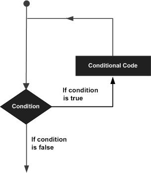
Структуры принятия решений требуют, чтобы программист указал одно или несколько условий, которые должны быть оценены или протестированы программой, вместе с оператором или инструкциями, которые должны быть выполнены, если условие определено как истинное, и, необязательно, другие операторы, которые должны быть выполнены, если условие определяется как ложное.
Ниже приводится общая форма типичной структуры принятия решений, встречающейся в большинстве языков программирования.

MATLAB предоставляет следующие типы заявлений о принятии решений. Нажмите на следующие ссылки, чтобы проверить их детали –
| Sr.No. | Заявление и описание |
|---|---|
| 1 | if … end
Оператор if … end состоит из логического выражения, за которым следует один или несколько операторов. |
| 2 | если … еще … конец заявления
За оператором if может следовать необязательный оператор else , который выполняется, когда логическое выражение имеет значение false. |
| 3 | Если … elseif … elseif … else … конец заявления
За оператором if может следовать один (или несколько) необязательных elseif … и оператор else , что очень полезно для проверки различных условий. |
| 4 | вложенные операторы if
Вы можете использовать один оператор if или elseif внутри другого оператора if или elseif . |
| 5 | заявление о переключении
Оператор switch позволяет проверять переменную на соответствие списку значений. |
| 6 | вложенные операторы switch
Вы можете использовать один оператор switch внутри другого оператора (ов) switch . |
Оператор if … end состоит из логического выражения, за которым следует один или несколько операторов.
За оператором if может следовать необязательный оператор else , который выполняется, когда логическое выражение имеет значение false.
За оператором if может следовать один (или несколько) необязательных elseif … и оператор else , что очень полезно для проверки различных условий.
Вы можете использовать один оператор if или elseif внутри другого оператора if или elseif .
Оператор switch позволяет проверять переменную на соответствие списку значений.
Вы можете использовать один оператор switch внутри другого оператора (ов) switch .
MATLAB – Типы петель
Может возникнуть ситуация, когда вам нужно выполнить блок кода несколько раз. Как правило, операторы выполняются последовательно. Первый оператор в функции выполняется первым, затем следует второй и так далее.
Языки программирования предоставляют различные управляющие структуры, которые допускают более сложные пути выполнения.
Оператор цикла позволяет нам выполнять оператор или группу операторов несколько раз, и в большинстве языков программирования ниже приводится общая форма инструкции цикла.
MATLAB предоставляет следующие типы циклов для обработки требований циклов. Нажмите на следующие ссылки, чтобы проверить их детали –
| Sr.No. | Тип и описание петли |
|---|---|
| 1 | в то время как цикл
Повторяет оператор или группу операторов, пока данное условие выполняется. Он проверяет условие перед выполнением тела цикла. |
| 2 | для цикла
Выполняет последовательность операторов несколько раз и сокращает код, который управляет переменной цикла. |
| 3 | вложенные циклы
Вы можете использовать один или несколько циклов внутри любого другого цикла. |
Повторяет оператор или группу операторов, пока данное условие выполняется. Он проверяет условие перед выполнением тела цикла.
Выполняет последовательность операторов несколько раз и сокращает код, который управляет переменной цикла.
Вы можете использовать один или несколько циклов внутри любого другого цикла.
Заявления о контроле цикла
Операторы управления циклом изменяют выполнение от его нормальной последовательности. Когда выполнение покидает область действия, все автоматические объекты, созданные в этой области, уничтожаются.
MATLAB поддерживает следующие управляющие операторы. Нажмите на следующие ссылки, чтобы проверить их детали.
| Sr.No. | Контрольное заявление и описание |
|---|---|
| 1 | заявление о нарушении
Завершает оператор цикла и передает выполнение в оператор, следующий сразу за циклом. |
| 2 | продолжить заявление
Заставляет петлю пропускать оставшуюся часть своего тела и немедленно проверять свое состояние перед повторением. |
Завершает оператор цикла и передает выполнение в оператор, следующий сразу за циклом.
Заставляет петлю пропускать оставшуюся часть своего тела и немедленно проверять свое состояние перед повторением.
MATLAB – Векторы
Вектор – это одномерный массив чисел. MATLAB позволяет создавать два типа векторов –
- Векторы строк
- Векторы столбцов
Строки Векторы
Векторы строк создаются путем заключения набора элементов в квадратных скобках с использованием пробела или запятой для разделения элементов.
Live Demo
r = [7 8 9 10 11]
MATLAB выполнит приведенный выше оператор и вернет следующий результат –
r =

   7    8    9   10   11
Векторы столбцов
Векторы столбцов создаются заключением набора элементов в квадратные скобки с использованием точки с запятой для разделения элементов.
Live Demo
c = [7; 8; 9; 10; 11]
MATLAB выполнит приведенный выше оператор и вернет следующий результат –
c =
      7
      8
      9
      10
      11
Ссылка на элементы вектора
Вы можете ссылаться на один или несколько элементов вектора несколькими способами. I- й компонент вектора v обозначается как v (i). Например –
Live Demo
v = [ 1; 2; 3; 4; 5; 6];	% creating a column vector of 6 elements
v(3)
MATLAB выполнит приведенный выше оператор и вернет следующий результат –
ans = 3
Когда вы ссылаетесь на вектор с двоеточием, например, v (:), в нем отображаются все компоненты вектора.
Live Demo
v = [ 1; 2; 3; 4; 5; 6];	% creating a column vector of 6 elements
v(:)
MATLAB выполнит приведенный выше оператор и вернет следующий результат –
ans =
     1
     2
     3
     4
     5
     6
MATLAB позволяет вам выбрать диапазон элементов из вектора.
Например, давайте создадим вектор-строку rv из 9 элементов, затем мы будем ссылаться на элементы с 3 по 7, написав rv (3: 7), и создадим новый вектор с именем sub_rv .
Live Demo
rv = [1 2 3 4 5 6 7 8 9];
sub_rv = rv(3:7)
MATLAB выполнит приведенный выше оператор и вернет следующий результат –
sub_rv =

   3   4   5   6   7
Векторные операции
В этом разделе давайте обсудим следующие векторные операции –
-
Сложение и вычитание векторов
-
Скалярное Умножение Векторов
-
Транспонирование вектора
-
Добавление векторов
-
Величина вектора
-
Вектор Дот Продукт
-
Векторы с равномерно расположенными элементами
Сложение и вычитание векторов
Скалярное Умножение Векторов
Транспонирование вектора
Добавление векторов
Величина вектора
Вектор Дот Продукт
Векторы с равномерно расположенными элементами
MATLAB – Матрица
Матрица – это двумерный массив чисел.
В MATLAB вы создаете матрицу, вводя элементы в каждой строке в виде чисел, разделенных запятыми или пробелами, и используя точки с запятой, чтобы отметить конец каждой строки.
Например, давайте создадим матрицу 4 на 5 a –
Live Demo
a = [ 1 2 3 4 5; 2 3 4 5 6; 3 4 5 6 7; 4 5 6 7 8]
MATLAB выполнит приведенный выше оператор и вернет следующий результат –
a =
      1     2     3     4     5
      2     3     4     5     6
      3     4     5     6     7
      4     5     6     7     8
Ссылка на элементы матрицы
Для ссылки на элемент в m- й строке и n- м столбце матрицы mx мы пишем:
mx(m, n);
Например, чтобы обратиться к элементу во 2- й строке и 5- м столбце матрицы a , как создано в последнем разделе, мы набираем –
Live Demo
a = [ 1 2 3 4 5; 2 3 4 5 6; 3 4 5 6 7; 4 5 6 7 8];
a(2,5)
MATLAB выполнит приведенный выше оператор и вернет следующий результат –
ans = 6
Для ссылки на все элементы в m- м столбце мы набираем A (:, m).
Создадим вектор-столбец v из элементов 4- й строки матрицы a –
Live Demo
a = [ 1 2 3 4 5; 2 3 4 5 6; 3 4 5 6 7; 4 5 6 7 8];
v = a(:,4)
MATLAB выполнит приведенный выше оператор и вернет следующий результат –
v =
      4
      5
      6
      7
Вы также можете выбрать элементы в столбцах с m по n, для этого мы напишем:
a(:,m:n)
Давайте создадим меньшую матрицу, взяв элементы из второго и третьего столбцов –
Live Demo
a = [ 1 2 3 4 5; 2 3 4 5 6; 3 4 5 6 7; 4 5 6 7 8];
a(:, 2:3)
MATLAB выполнит приведенный выше оператор и вернет следующий результат –
ans =
      2     3
      3     4
      4     5
      5     6
Таким же образом вы можете создать подматрицу, взяв подчасть матрицы.
Live Demo
a = [ 1 2 3 4 5; 2 3 4 5 6; 3 4 5 6 7; 4 5 6 7 8];
a(:, 2:3)
MATLAB выполнит приведенный выше оператор и вернет следующий результат –
ans =
      2     3
      3     4
      4     5
      5     6
Таким же образом вы можете создать подматрицу, взяв подчасть матрицы.
Например, давайте создадим подматрицу sa, взяв внутреннюю часть a –
3     4     5
4     5     6
Для этого напишите –
Live Demo
a = [ 1 2 3 4 5; 2 3 4 5 6; 3 4 5 6 7; 4 5 6 7 8];
sa = a(2:3,2:4)
MATLAB выполнит приведенный выше оператор и вернет следующий результат –
sa =
      3     4     5
      4     5     6
Удаление строки или столбца в матрице
Вы можете удалить всю строку или столбец матрицы, назначив пустой набор квадратных скобок [] для этой строки или столбца. По сути, [] обозначает пустой массив.
Например, давайте удалим четвертый ряд –
Live Demo
a = [ 1 2 3 4 5; 2 3 4 5 6; 3 4 5 6 7; 4 5 6 7 8];
a( 4 , : ) = []
MATLAB выполнит приведенный выше оператор и вернет следующий результат –
a =
      1     2     3     4     5
      2     3     4     5     6
      3     4     5     6     7
Далее, давайте удалим пятый столбец –
Live Demo
a = [ 1 2 3 4 5; 2 3 4 5 6; 3 4 5 6 7; 4 5 6 7 8];
a(: , 5)=[]
MATLAB выполнит приведенный выше оператор и вернет следующий результат –
a =
      1     2     3     4
      2     3     4     5
      3     4     5     6
      4     5     6     7
пример
В этом примере давайте создадим матрицу 3 на 3 m, затем дважды скопируем вторую и третью строки этой матрицы, чтобы создать матрицу 4 на 3.
Создайте файл сценария со следующим кодом –
Live Demo
a = [ 1 2 3 ; 4 5 6; 7 8 9];
new_mat = a([2,3,2,3],:)
Когда вы запускаете файл, он показывает следующий результат –
new_mat =
      4     5     6
      7     8     9
      4     5     6
      7     8     9
Матричные Операции
В этом разделе давайте обсудим следующие основные и часто используемые матричные операции –
-
Сложение и вычитание матриц
-
Отдел матриц
-
Скалярные операции матриц
-
Транспонировать матрицы
-
Конкатенирующие матрицы
-
Умножение матриц
-
Определитель матрицы
-
Инверсия матрицы
Сложение и вычитание матриц
Отдел матриц
Скалярные операции матриц
Транспонировать матрицы
Конкатенирующие матрицы
Умножение матриц
Определитель матрицы
Инверсия матрицы
MATLAB – Массивы
Все переменные всех типов данных в MATLAB являются многомерными массивами. Вектор – это одномерный массив, а матрица – это двумерный массив.
Мы уже обсуждали векторы и матрицы. В этой главе мы обсудим многомерные массивы. Однако перед этим давайте обсудим некоторые специальные типы массивов.
Специальные массивы в MATLAB
В этом разделе мы обсудим некоторые функции, которые создают специальные массивы. Для всех этих функций один аргумент создает квадратный массив, двойные аргументы создают прямоугольный массив.
Функция нулей () создает массив всех нулей –
Например –
Live Demo
zeros(5)
MATLAB выполнит приведенный выше оператор и вернет следующий результат –
ans =
      0     0     0     0     0
      0     0     0     0     0
      0     0     0     0     0
      0     0     0     0     0
      0     0     0     0     0
Функция ones () создает массив всех единиц –
Например –
Live Demo
ones(4,3)
MATLAB выполнит приведенный выше оператор и вернет следующий результат –
ans =
      1     1     1
      1     1     1
      1     1     1
      1     1     1
Функция eye () создает единичную матрицу.
Например –
Live Demo
eye(4)
MATLAB выполнит приведенный выше оператор и вернет следующий результат –
ans =
      1     0     0     0
      0     1     0     0
      0     0     1     0
      0     0     0     1
Функция rand () создает массив равномерно распределенных случайных чисел по (0,1) –
Например –
Live Demo
rand(3, 5)
MATLAB выполнит приведенный выше оператор и вернет следующий результат –
ans =
   0.8147    0.9134    0.2785    0.9649    0.9572
   0.9058    0.6324    0.5469    0.1576    0.4854
   0.1270    0.0975    0.9575    0.9706    0.8003
Магический Квадрат
Магический квадрат – это квадрат, который дает одинаковую сумму, когда его элементы добавляются построчно, по столбцам или по диагонали.
Функция magic () создает массив магических квадратов. Требуется исключительный аргумент, который дает размер квадрата. Аргумент должен быть скаляром, большим или равным 3.
Live Demo
magic(4)
MATLAB выполнит приведенный выше оператор и вернет следующий результат –
ans =
   16     2     3    13
   5    11    10     8
   9     7     6    12
   4    14    15     1
Многомерные массивы
В MATLAB массив, имеющий более двух измерений, называется многомерным массивом. Многомерные массивы в MATLAB являются расширением нормальной двумерной матрицы.
Обычно для создания многомерного массива мы сначала создаем двумерный массив и расширяем его.
Например, давайте создадим двумерный массив a.
Live Demo
a = [7 9 5; 6 1 9; 4 3 2]
MATLAB выполнит приведенный выше оператор и вернет следующий результат –
a =
   7     9     5
   6     1     9
   4     3     2
Массив a является массивом 3 на 3; мы можем добавить третье измерение к, предоставив такие значения, как –
Live Demo
a(:, :, 2)= [ 1 2 3; 4 5 6; 7 8 9]
MATLAB выполнит приведенный выше оператор и вернет следующий результат –
a =

ans(:,:,1) =

   0   0   0
   0   0   0
   0   0   0

ans(:,:,2) =

   1   2   3
   4   5   6
   7   8   9
Мы также можем создавать многомерные массивы, используя функции ones (), zeros () или rand ().
Например,
Live Demo
b = rand(4,3,2)
MATLAB выполнит приведенный выше оператор и вернет следующий результат –
b(:,:,1) =
   0.0344    0.7952    0.6463
   0.4387    0.1869    0.7094
   0.3816    0.4898    0.7547
   0.7655    0.4456    0.2760

b(:,:,2) =
   0.6797    0.4984    0.2238
   0.6551    0.9597    0.7513
   0.1626    0.3404    0.2551
   0.1190    0.5853    0.5060
Мы также можем использовать функцию cat () для построения многомерных массивов. Он объединяет список массивов по указанному измерению –
Синтаксис для функции cat () –
B = cat(dim, A1, A2...)
Куда,
-
B – новый созданный массив
-
A1 , A2 , … массивы, которые будут объединены
-
dim – это размер, по которому объединяются массивы.
B – новый созданный массив
A1 , A2 , … массивы, которые будут объединены
dim – это размер, по которому объединяются массивы.
пример
Создайте файл сценария и введите в него следующий код –
Live Demo
a = [9 8 7; 6 5 4; 3 2 1];
b = [1 2 3; 4 5 6; 7 8 9];
c = cat(3, a, b, [ 2 3 1; 4 7 8; 3 9 0])
Когда вы запускаете файл, он отображает –
c(:,:,1) =
      9     8     7
      6     5     4
      3     2     1
c(:,:,2) =
      1     2     3
      4     5     6
      7     8     9
c(:,:,3) =
      2     3     1
      4     7     8
      3     9     0
Функции массива
MATLAB предоставляет следующие функции для сортировки, вращения, перестановки, изменения формы или смещения содержимого массива.
| функция | Цель |
|---|---|
| длина | Длина вектора или наибольшее измерение массива |
| ndims | Количество размеров массива |
| numel | Количество элементов массива |
| размер | Размеры массива |
| iscolumn | Определяет, является ли ввод вектором столбца |
| пустой | Определяет, является ли массив пустым |
| ismatrix | Определяет, является ли ввод матричным |
| isrow | Определяет, является ли ввод вектором строки |
| isscalar | Определяет, является ли вход скалярным |
| isvector | Определяет, является ли входной вектор |
| blkdiag | Создает блочную диагональную матрицу из входных аргументов. |
| circshift | Смещает массив по кругу |
| ctranspose | Комплексное сопряженное транспонирование |
| диаг | Диагональные матрицы и диагонали матрицы |
| flipdim | Переворачивает массив по указанному измерению |
| fliplr | Отразить матрицу слева направо |
| flipud | Переворачивает матрицу вверх-вниз |
| ipermute | Инвертирует перестановочные размеры массива ND |
| переставлять | Переставляет размеры массива ND |
| repmat | Реплики и массив плиток |
| перекроить | Перекраивает массив |
| rot90 | Поворот матрицы на 90 градусов |
| shiftdim | Смещает размеры |
| issorted | Определяет, находятся ли заданные элементы в отсортированном порядке |
| Сортировать | Сортирует элементы массива в порядке возрастания или убывания |
| sortrows | Сортирует строки в порядке возрастания |
| выжимать | Удаляет одиночные размеры |
| транспонировать | транспонировать |
| векторизовать | Векторизованное выражение |
Примеры
Следующие примеры иллюстрируют некоторые из функций, упомянутых выше.
Длина, Размер и Количество элементов –
Создайте файл сценария и введите в него следующий код –
Live Demo
x = [7.1, 3.4, 7.2, 28/4, 3.6, 17, 9.4, 8.9];
length(x)      % length of x vector
y = rand(3, 4, 5, 2);
ndims(y)       % no of dimensions in array y
s = ['Zara', 'Nuha', 'Shamim', 'Riz', 'Shadab'];
numel(s)       % no of elements in s
Когда вы запускаете файл, он показывает следующий результат –
ans =  8
ans =  4
ans =  23
Круговое смещение элементов массива –
Создайте файл сценария и введите в него следующий код –
Live Demo
a = [1 2 3; 4 5 6; 7 8 9]  % the original array a
b = circshift(a,1)         %  circular shift first dimension values down by 1.
c = circshift(a,[1 -1])    % circular shift first dimension values % down by 1
                           % and second dimension values to the left % by 1.
Когда вы запускаете файл, он показывает следующий результат –
a =
   1     2     3
   4     5     6
   7     8     9

b =
   7     8     9
   1     2     3
   4     5     6

c =
   8     9     7
   2     3     1
   5     6     4
Сортировка массивов
Создайте файл сценария и введите в него следующий код –
Live Demo
v = [ 23 45 12 9 5 0 19 17]  % horizontal vector
sort(v)                      % sorting v
m = [2 6 4; 5 3 9; 2 0 1]    % two dimensional array
sort(m, 1)                   % sorting m along the row
sort(m, 2)                   % sorting m along the column
Когда вы запускаете файл, он показывает следующий результат –
v =
   23    45    12     9     5     0    19    17
ans =
   0     5     9    12    17    19    23    45
m =
   2     6     4
   5     3     9
   2     0     1
ans =
   2     0     1
   2     3     4
   5     6     9
ans =
   2     4     6
   3     5     9
   0     1     2
Cell Array
Массивы ячеек – это массивы индексированных ячеек, где каждая ячейка может хранить массив разных измерений и типов данных.
Функция cell используется для создания массива cell. Синтаксис для функции ячейки –
C = cell(dim)
C = cell(dim1,...,dimN)
D = cell(obj)
Куда,
-
С – массив ячеек;
-
dim – скалярное целое число или вектор целых чисел, который определяет размеры массива ячеек C;
-
dim1, …, dimN – скалярные целые числа, которые определяют размеры C;
-
obj является одним из следующих –
- Массив или объект Java
- .NET массив типа System.String или System.Object
С – массив ячеек;
dim – скалярное целое число или вектор целых чисел, который определяет размеры массива ячеек C;
dim1, …, dimN – скалярные целые числа, которые определяют размеры C;
obj является одним из следующих –
пример
Создайте файл сценария и введите в него следующий код –
Live Demo
c = cell(2, 5);
c = {'Red', 'Blue', 'Green', 'Yellow', 'White'; 1 2 3 4 5}
Когда вы запускаете файл, он показывает следующий результат –
c =
{
   [1,1] = Red
   [2,1] =  1
   [1,2] = Blue
   [2,2] =  2
   [1,3] = Green
   [2,3] =  3
   [1,4] = Yellow
   [2,4] =  4
   [1,5] = White
   [2,5] =  5
}
Доступ к данным в массивах ячеек
Существует два способа обращения к элементам массива ячеек:
- Заключение индексов в первую скобку () для ссылки на наборы ячеек
- Заключение индексов в фигурные скобки {} для ссылки на данные в отдельных ячейках
Когда вы заключаете индексы в первую скобку, это относится к набору ячеек.
Индексы массива ячеек в гладких скобках относятся к наборам ячеек.
Например –
Live Demo
c = {'Red', 'Blue', 'Green', 'Yellow', 'White'; 1 2 3 4 5};
c(1:2,1:2)
MATLAB выполнит приведенный выше оператор и вернет следующий результат –
ans =
{
   [1,1] = Red
   [2,1] =  1
   [1,2] = Blue
   [2,2] =  2
}
Вы также можете получить доступ к содержимому ячеек путем индексации с помощью фигурных скобок.
Например –
Live Demo
c = {'Red', 'Blue', 'Green', 'Yellow', 'White'; 1 2 3 4 5};
c{1, 2:4}
MATLAB выполнит приведенный выше оператор и вернет следующий результат –
ans = Blue
ans = Green
ans = Yellow
MATLAB – двоеточие
Двоеточие (:) является одним из самых полезных операторов в MATLAB. Он используется для создания векторов, массивов индексов и определения для итераций .
Если вы хотите создать вектор строки, содержащий целые числа от 1 до 10, вы пишете –
Live Demo
1:10
MATLAB выполняет инструкцию и возвращает вектор строки, содержащий целые числа от 1 до 10 –
ans =

   1    2    3    4    5    6    7    8    9   10
Если вы хотите указать значение приращения, отличное от единицы, например:
Live Demo
100: -5: 50
MATLAB выполняет инструкцию и возвращает следующий результат –
ans =
   100    95    90    85    80    75    70    65    60    55    50
Давайте возьмем другой пример –
Live Demo
0:pi/8:pi
MATLAB выполняет инструкцию и возвращает следующий результат –
ans =
   Columns 1 through 7
      0    0.3927    0.7854    1.1781    1.5708    1.9635    2.3562
   Columns 8 through 9
      2.7489    3.1416
Вы можете использовать оператор двоеточия, чтобы создать вектор индексов для выбора строк, столбцов или элементов массивов.
Следующая таблица описывает его использование для этой цели (у нас есть матрица A) –
| Формат | Цель |
|---|---|
| А (:, J) | это j-й столбец А. |
| А (я, 🙂 | это шестой ряд А. |
| А (:, 🙂 | эквивалентный двумерный массив Для матриц это то же самое, что и A. |
| А (J: к) | является A (j), A (j + 1), …, A (k). |
| A (:, J: к) | является A (:, j), A (:, j + 1), …, A (:, k). |
| А (:,:, к) | является k- й страницей трехмерного массива A. |
| A (I, J, K, 🙂 | является вектором в четырехмерном массиве A. Вектор включает в себя A (i, j, k, 1), A (i, j, k, 2), A (i, j, k, 3) и так далее. |
| А (:) | это все элементы А, рассматриваемые как один столбец. В левой части оператора присваивания A (:) заполняет A, сохраняя свою форму ранее. В этом случае правая сторона должна содержать то же количество элементов, что и A. |
пример
Создайте файл сценария и введите в нем следующий код –
Live Demo
A = [1 2 3 4; 4 5 6 7; 7 8 9 10]
A(:,2)      % second column of A
A(:,2:3)    % second and third column of A
A(2:3,2:3)  % second and third rows and second and third columns
Когда вы запускаете файл, он показывает следующий результат –
A =
      1     2     3     4
      4     5     6     7
      7     8     9    10

ans =
      2
      5
      8

ans =
      2     3
      5     6
      8     9

ans =
      5     6
      8     9
MATLAB – Числа
MATLAB поддерживает различные числовые классы, которые включают целые числа со знаком и без знака, а также числа с плавающей запятой одинарной и двойной точности. По умолчанию MATLAB сохраняет все числовые значения как числа с плавающей запятой двойной точности.
Вы можете сохранить любое число или массив чисел в виде целых чисел или чисел одинарной точности.
Все числовые типы поддерживают базовые операции с массивами и математические операции.
Преобразование в различные числовые типы данных
MATLAB предоставляет следующие функции для преобразования в различные числовые типы данных –
| функция | Цель |
|---|---|
| двойной | Преобразует в число с двойной точностью |
| не замужем | Преобразует в число с одинарной точностью |
| int8 | Преобразует в 8-разрядное целое число со знаком |
| int16 | Преобразует в 16-разрядное целое число со знаком |
| int32 | Преобразует в 32-разрядное целое число со знаком |
| int64 | Преобразует в 64-разрядное целое число со знаком |
| uint8 | Преобразует в 8-разрядное целое число без знака |
| uint16 | Преобразует в 16-разрядное целое число без знака |
| uint32 | Преобразует в 32-разрядное целое число без знака |
| uint64 | Преобразует в 64-разрядное целое число без знака |
пример
Создайте файл сценария и введите следующий код –
Live Demo
x = single([5.32 3.47 6.28]) .* 7.5
x = double([5.32 3.47 6.28]) .* 7.5
x = int8([5.32 3.47 6.28]) .* 7.5
x = int16([5.32 3.47 6.28]) .* 7.5
x = int32([5.32 3.47 6.28]) .* 7.5
x = int64([5.32 3.47 6.28]) .* 7.5
Когда вы запускаете файл, он показывает следующий результат –
x =

   39.900   26.025   47.100

x =

   39.900   26.025   47.100

x =

   38  23  45

x =

   38  23  45

x =

   38  23  45

x =

   38  23  45
пример
Давайте расширим предыдущий пример немного подробнее. Создайте файл сценария и введите следующий код –
Live Demo
x = int32([5.32 3.47 6.28]) .* 7.5
x = int64([5.32 3.47 6.28]) .* 7.5
x = num2cell(x)
Когда вы запускаете файл, он показывает следующий результат –
x =

   38  23  45

x =

   38  23  45

x =
{
   [1,1] = 38
   [1,2] = 23
   [1,3] = 45
}
Самые маленькие и самые большие целые числа
Функции intmax () и intmin () возвращают максимальное и минимальное значения, которые могут быть представлены всеми типами целых чисел.
Обе функции принимают в качестве аргумента целочисленный тип данных, например, intmax (int8) или intmin (int64), и возвращают максимальное и минимальное значения, которые вы можете представить в целочисленном типе данных.
пример
В следующем примере показано, как получить наименьшее и наибольшее значения целых чисел. Создайте файл сценария и напишите в нем следующий код –
Live Demo
% displaying the smallest and largest signed integer data
str = 'The range for int8 is:nt%d to %d ';
sprintf(str, intmin('int8'), intmax('int8'))
str = 'The range for int16 is:nt%d to %d ';
sprintf(str, intmin('int16'), intmax('int16'))
str = 'The range for int32 is:nt%d to %d ';
sprintf(str, intmin('int32'), intmax('int32'))
str = 'The range for int64 is:nt%d to %d ';
sprintf(str, intmin('int64'), intmax('int64'))

% displaying the smallest and largest unsigned integer data
str = 'The range for uint8 is:nt%d to %d ';
sprintf(str, intmin('uint8'), intmax('uint8'))
str = 'The range for uint16 is:nt%d to %d ';
sprintf(str, intmin('uint16'), intmax('uint16'))
str = 'The range for uint32 is:nt%d to %d ';
sprintf(str, intmin('uint32'), intmax('uint32'))
str = 'The range for uint64 is:nt%d to %d ';
sprintf(str, intmin('uint64'), intmax('uint64'))
Когда вы запускаете файл, он показывает следующий результат –
ans = The range for int8 is:
	-128 to 127
ans = The range for int16 is:
	-32768 to 32767
ans = The range for int32 is:
	-2147483648 to 2147483647
ans = The range for int64 is:
	0 to 0
ans = The range for uint8 is:
	0 to 255
ans = The range for uint16 is:
	0 to 65535
ans = The range for uint32 is:
	0 to -1
ans = The range for uint64 is:
	0 to 18446744073709551616
Самые маленькие и самые большие числа с плавающей точкой
Функции realmax () и realmin () возвращают максимальное и минимальное значения, которые могут быть представлены числами с плавающей запятой.
Обе функции при вызове с аргументом ‘single’ возвращают максимальное и минимальное значения, которые вы можете представить с помощью типа данных с одинарной точностью, а при вызове с аргументом ‘double’ возвращают максимальное и минимальное значения, которые вы можете представить с помощью тип данных двойной точности.
пример
В следующем примере показано, как получить наименьшее и наибольшее числа с плавающей запятой. Создайте файл сценария и напишите в нем следующий код –
Live Demo
% displaying the smallest and largest single-precision
% floating point number
str = 'The range for single is:nt%g to %g andnt %g to  %g';
sprintf(str, -realmax('single'), -realmin('single'), ...
   realmin('single'), realmax('single'))

% displaying the smallest and largest double-precision
% floating point number
str = 'The range for double is:nt%g to %g andnt %g to  %g';
sprintf(str, -realmax('double'), -realmin('double'), ...
   realmin('double'), realmax('double'))
Когда вы запускаете файл, он показывает следующий результат –
ans = The range for single is:
        -3.40282e+38 to -1.17549e-38 and
         1.17549e-38 to  3.40282e+38
ans = The range for double is:
        -1.79769e+308 to -2.22507e-308 and
         2.22507e-308 to  1.79769e+308
MATLAB – Струны
Создать строку символов в MATLAB довольно просто. На самом деле, мы использовали это много раз. Например, вы вводите следующее в командной строке –
Live Demo
my_string = 'Tutorials Point'
MATLAB выполнит приведенный выше оператор и вернет следующий результат –
my_string = Tutorials Point
MATLAB рассматривает все переменные как массивы, а строки – как символьные массивы. Давайте используем команду whos для проверки созданной выше переменной –
whos
MATLAB выполнит приведенный выше оператор и вернет следующий результат –
Name           Size            Bytes  Class    Attributes
my_string      1x16               32  char
Интересно, что вы можете использовать функции преобразования чисел, такие как uint8 или uint16, чтобы преобразовать символы в строке в их числовые коды. Функция char преобразует вектор целых чисел обратно в символы –
пример
Создайте файл сценария и введите в него следующий код –
Live Demo
my_string = 'Tutorial''s Point';
str_ascii = uint8(my_string)        % 8-bit ascii values
str_back_to_char= char(str_ascii)
str_16bit = uint16(my_string)       % 16-bit ascii values
str_back_to_char = char(str_16bit)
Когда вы запускаете файл, он показывает следующий результат –
str_ascii =

   84  117  116  111  114  105   97  108   39  115   32   80  111  105  110  116

str_back_to_char = Tutorial's Point
str_16bit =

   84  117  116  111  114  105   97  108   39  115   32   80  111  105  110  116

str_back_to_char = Tutorial's Point
Прямоугольный массив символов
Строки, которые мы обсуждали до сих пор, являются одномерными символьными массивами; Однако нам нужно хранить больше, чем это. Нам нужно хранить более объемные текстовые данные в нашей программе. Это достигается путем создания прямоугольных массивов символов.
Простейший способ создания прямоугольного массива символов состоит в объединении двух или более одномерных массивов символов по вертикали или по горизонтали, как требуется.
Вы можете комбинировать строки по вертикали одним из следующих способов –
-
Используя оператор конкатенации MATLAB [] и разделяя каждую строку точкой с запятой (;). Обратите внимание, что в этом методе каждая строка должна содержать одинаковое количество символов. Для строк разной длины вы должны заполнять пробелами по мере необходимости.
-
Использование функции char . Если строки имеют разную длину, более короткие строки облагаются символьными символами, чтобы в каждой строке было одинаковое количество символов.
Используя оператор конкатенации MATLAB [] и разделяя каждую строку точкой с запятой (;). Обратите внимание, что в этом методе каждая строка должна содержать одинаковое количество символов. Для строк разной длины вы должны заполнять пробелами по мере необходимости.
Использование функции char . Если строки имеют разную длину, более короткие строки облагаются символьными символами, чтобы в каждой строке было одинаковое количество символов.
пример
Создайте файл сценария и введите в него следующий код –
Live Demo
doc_profile = ['Zara Ali                             '; ...
               'Sr. Surgeon                          '; ...
               'R N Tagore Cardiology Research Center']
doc_profile = char('Zara Ali', 'Sr. Surgeon', ...
                  'RN Tagore Cardiology Research Center')
Когда вы запускаете файл, он показывает следующий результат –
doc_profile =
Zara Ali
Sr. Surgeon
R N Tagore Cardiology Research Center
doc_profile =
Zara Ali
Sr. Surgeon
RN Tagore Cardiology Research Center
Вы можете комбинировать строки горизонтально одним из следующих способов –
-
Используя оператор конкатенации MATLAB, [] и разделяя входные строки запятой или пробелом. Этот метод сохраняет любые конечные пробелы во входных массивах.
-
Используя функцию конкатенации строк, strcat . Этот метод удаляет завершающие пробелы во входных данных.
Используя оператор конкатенации MATLAB, [] и разделяя входные строки запятой или пробелом. Этот метод сохраняет любые конечные пробелы во входных массивах.
Используя функцию конкатенации строк, strcat . Этот метод удаляет завершающие пробелы во входных данных.
пример
Создайте файл сценария и введите в него следующий код –
Live Demo
name =     'Zara Ali                             ';
position = 'Sr. Surgeon                          ';
worksAt =  'R N Tagore Cardiology Research Center';
profile = [name ', ' position ', ' worksAt]
profile = strcat(name, ', ', position, ', ', worksAt)
Когда вы запускаете файл, он показывает следующий результат –
profile = Zara Ali      , Sr. Surgeon      , R N Tagore Cardiology Research Center
profile = Zara Ali,Sr. Surgeon,R N Tagore Cardiology Research Center
Объединение строк в массив ячеек
Из нашего предыдущего обсуждения ясно, что объединение строк разной длины может быть проблематичным, поскольку все строки в массиве должны быть одинаковой длины. Мы использовали пробелы в конце строк, чтобы выровнять их длину.
Однако более эффективный способ объединения строк – преобразование полученного массива в массив ячеек.
Массив ячеек MATLAB может содержать различные размеры и типы данных в массиве. Массивы ячеек обеспечивают более гибкий способ хранения строк различной длины.
Функция cellstr преобразует массив символов в массив строк.
пример
Создайте файл сценария и введите в него следующий код –
Live Demo
name =     'Zara Ali                             ';
position = 'Sr. Surgeon                          ';
worksAt =  'R N Tagore Cardiology Research Center';
profile = char(name, position, worksAt);
profile = cellstr(profile);
disp(profile)
Когда вы запускаете файл, он показывает следующий результат –
{
   [1,1] = Zara Ali
   [2,1] = Sr. Surgeon
   [3,1] = R N Tagore Cardiology Research Center
}
Строковые функции в MATLAB
MATLAB предоставляет множество строковых функций для создания, объединения, анализа, сравнения и манипулирования строками.
В следующей таблице приведено краткое описание строковых функций в MATLAB –
| функция | Цель |
|---|---|
| Функции для хранения текста в символьных массивах, комбинирования символьных массивов и т. Д. | |
| заготовки | Создать строку пустых символов |
| cellstr | Создать массив строк из массива символов |
| голец | Преобразовать в массив символов (строку) |
| iscellstr | Определите, является ли ввод массивом строк |
| ischar | Определить, является ли элемент массивом символов |
| Sprintf | Форматировать данные в строку |
| strcat | Конкатенация строк по горизонтали |
| strjoin | Соединить строки в массиве ячеек в одну строку |
| Функции для идентификации частей строк, поиска и замены подстрок | |
| ischar | Определить, является ли элемент массивом символов |
| isletter | Элементы массива, которые являются буквенными буквами |
| isspace | Элементы массива, которые являются пробелами |
| isstrprop | Определить, относится ли строка к указанной категории |
| sscanf | Считать отформатированные данные из строки |
| strfind | Найти одну строку в другой |
| strrep | Найти и заменить подстроку |
| strsplit | Разделить строку по указанному разделителю |
| strtok | Отдельные части строки |
| validatestring | Проверьте правильность текстовой строки |
| symvar | Определить символические переменные в выражении |
| регулярное выражение | Соответствие регулярному выражению (с учетом регистра) |
| regexpi | Соответствие регулярному выражению (без учета регистра) |
| regexprep | Заменить строку с помощью регулярного выражения |
| regexptranslate | Перевести строку в регулярное выражение |
| Функции для сравнения строк | |
| зЬгстр | Сравнить строки (с учетом регистра) |
| strcmpi | Сравнить строки (без учета регистра) |
| strncmp | Сравните первые n символов строк (с учетом регистра) |
| strncmpi | Сравните первые n символов строк (без учета регистра) |
| Функции для изменения строки в верхний или нижний регистр, создания или удаления пробела | |
| deblank | Снять задние заготовки с конца струны |
| strtrim | Удалить начальные и конечные пробелы из строки |
| ниже | Преобразовать строку в нижний регистр |
| верхний | Преобразовать строку в верхний регистр |
| strjust | Обоснуйте массив символов |
Примеры
Следующие примеры иллюстрируют некоторые из вышеупомянутых строковых функций –
Форматирование строк
Создайте файл сценария и введите в него следующий код –
Live Demo
A = pi*1000*ones(1,5);
sprintf(' %f n %.2f n %+.2f n %12.2f n %012.2f n', A)
Когда вы запускаете файл, он показывает следующий результат –
ans =  3141.592654
   3141.59
   +3141.59
      3141.59
   000003141.59
Строки соединения
Создайте файл сценария и введите в него следующий код –
Live Demo
%cell array of strings
str_array = {'red','blue','green', 'yellow', 'orange'};

% Join strings in cell array into single string
str1 = strjoin(str_array, "-")
str2 = strjoin(str_array, ",")
Когда вы запускаете файл, он показывает следующий результат –
str1 = red-blue-green-yellow-orange
str2 = red,blue,green,yellow,orange
Поиск и замена строк
Создайте файл сценария и введите в него следующий код –
Live Demo
students = {'Zara Ali', 'Neha Bhatnagar', ...
            'Monica Malik', 'Madhu Gautam', ...
            'Madhu Sharma', 'Bhawna Sharma',...
            'Nuha Ali', 'Reva Dutta', ...
            'Sunaina Ali', 'Sofia Kabir'};

% The strrep function searches and replaces sub-string.
new_student = strrep(students(8), 'Reva', 'Poulomi')
% Display first names
first_names = strtok(students)
Когда вы запускаете файл, он показывает следующий результат –
new_student =
{
   [1,1] = Poulomi Dutta
}
first_names =
{
   [1,1] = Zara
   [1,2] = Neha
   [1,3] = Monica
   [1,4] = Madhu
   [1,5] = Madhu
   [1,6] = Bhawna
   [1,7] = Nuha
   [1,8] = Reva
   [1,9] = Sunaina
   [1,10] = Sofia
}
Сравнение строк
Создайте файл сценария и введите в него следующий код –
Live Demo
str1 = 'This is test'
str2 = 'This is text'
if (strcmp(str1, str2))
   sprintf('%s and %s are equal', str1, str2)
else
   sprintf('%s and %s are not equal', str1, str2)
end
Когда вы запускаете файл, он показывает следующий результат –
str1 = This is test
str2 = This is text
ans = This is test and This is text are not equal
MATLAB – Функции
Функция – это группа операторов, которые вместе выполняют задачу. В MATLAB функции определены в отдельных файлах. Имя файла и функции должны совпадать.
Функции работают с переменными в их собственном рабочем пространстве, которое также называется локальным рабочим пространством , отдельно от рабочего пространства, к которому вы обращаетесь в командной строке MATLAB, которое называется базовым рабочим пространством .
Функции могут принимать более одного входного аргумента и могут возвращать более одного выходного аргумента.
Синтаксис оператора функции –
function [out1,out2, ..., outN] = myfun(in1,in2,in3, ..., inN)
пример
Следующая функция с именем mymax должна быть записана в файл с именем mymax.m . Он принимает пять чисел в качестве аргумента и возвращает максимум чисел.
Создайте файл функции с именем mymax.m и введите в него следующий код –
function max = mymax(n1, n2, n3, n4, n5)

%This function calculates the maximum of the
% five numbers given as input
max =  n1;
if(n2 > max)
   max = n2;
end
if(n3 > max)
   max = n3;
end
if(n4 > max)
   max = n4;
end
if(n5 > max)
   max = n5;
end
Первая строка функции начинается с ключевого слова function . Это дает название функции и порядок аргументов. В нашем примере функция mymax имеет пять входных аргументов и один выходной аргумент.
Строки комментариев, которые идут сразу после оператора функции, содержат текст справки. Эти строки печатаются при вводе –
help mymax
MATLAB выполнит приведенный выше оператор и вернет следующий результат –
This function calculates the maximum of the
   five numbers given as input
Вы можете вызвать функцию как –
mymax(34, 78, 89, 23, 11)
MATLAB выполнит приведенный выше оператор и вернет следующий результат –
ans = 89
Анонимные функции
Анонимная функция похожа на встроенную функцию в традиционных языках программирования, определенную в одной инструкции MATLAB. Он состоит из одного выражения MATLAB и любого количества входных и выходных аргументов.
Вы можете определить анонимную функцию прямо в командной строке MATLAB или в функции или скрипте.
Таким образом, вы можете создавать простые функции без необходимости создавать файл для них.
Синтаксис для создания анонимной функции из выражения:
f = @(arglist)expression
пример
В этом примере мы напишем анонимную функцию с именем power, которая будет принимать два числа в качестве входных данных и возвращать первое число, возведенное в степень второго числа.
Создайте файл сценария и введите в нем следующий код –
Live Demo
power = @(x, n) x.^n;
result1 = power(7, 3)
result2 = power(49, 0.5)
result3 = power(10, -10)
result4 = power (4.5, 1.5)
Когда вы запускаете файл, он отображает –
result1 =  343
result2 =  7
result3 =  1.0000e-10
result4 =  9.5459
Основные и подфункции
Любая функция, кроме анонимной, должна быть определена в файле. Каждый файл функции содержит требуемую первичную функцию, которая появляется первой, и любое количество необязательных подфункций, которые идут после основной функции и используются ею.
Первичные функции могут быть вызваны из-за пределов файла, который их определяет, либо из командной строки, либо из других функций, но подфункции не могут быть вызваны из командной строки или других функций вне файла функции.
Подфункции видны только основной функции и другим подфункциям в файле функций, который их определяет.
пример
Напишем функцию с именем quadratic, которая будет вычислять корни квадратного уравнения. Функция будет принимать три входа: квадратичный коэффициент, линейный коэффициент и постоянный член. Это вернуло бы корни.
Файл функций quadratic.m будет содержать основную функцию quadratic и вспомогательный диск , который вычисляет дискриминант.
Создайте файл функции quadratic.m и введите в него следующий код –
function [x1,x2] = quadratic(a,b,c)

%this function returns the roots of
% a quadratic equation.
% It takes 3 input arguments
% which are the co-efficients of x2, x and the
%constant term
% It returns the roots
d = disc(a,b,c);
x1 = (-b + d) / (2*a);
x2 = (-b - d) / (2*a);
end   % end of quadratic

function dis = disc(a,b,c)
%function calculates the discriminant
dis = sqrt(b^2 - 4*a*c);
end   % end of sub-function
Вы можете вызвать вышеуказанную функцию из командной строки как –
quadratic(2,4,-4)
MATLAB выполнит приведенный выше оператор и вернет следующий результат –
ans = 0.7321
Вложенные функции
Вы можете определить функции в теле другой функции. Это так называемые вложенные функции. Вложенная функция содержит любой или все компоненты любой другой функции.
Вложенные функции определены в области действия другой функции и имеют общий доступ к рабочему пространству содержащей функции.
Вложенная функция имеет следующий синтаксис:
function x = A(p1, p2)
...
B(p2)
   function y = B(p3)
   ...
   end
...
end
пример
Перепишем функцию quadratic из предыдущего примера, однако на этот раз функция диска будет вложенной функцией.
Создайте файл функции quadratic2.m и введите в него следующий код –
function [x1,x2] = quadratic2(a,b,c)
function disc  % nested function
d = sqrt(b^2 - 4*a*c);
end   % end of function disc

disc;
x1 = (-b + d) / (2*a);
x2 = (-b - d) / (2*a);
end   % end of function quadratic2
Вы можете вызвать вышеуказанную функцию из командной строки как –
quadratic2(2,4,-4)
MATLAB выполнит приведенный выше оператор и вернет следующий результат –
ans = 0.73205
Частные функции
Закрытая функция – это основная функция, которая видна только ограниченной группе других функций. Если вы не хотите показывать реализацию функции (й), вы можете создать их как частные функции.
Закрытые функции находятся в подпапках со специальным именем private .
Они видны только функциям в родительской папке.
пример
Перепишем квадратичную функцию. На этот раз, однако, функция диска, вычисляющая дискриминант, будет частной функцией.
Создайте подпапку с именем private в рабочем каталоге. Сохраните в нем следующий файл функции disc.m –
function dis = disc(a,b,c)
%function calculates the discriminant
dis = sqrt(b^2 - 4*a*c);
end      % end of sub-function
Создайте функцию quadratic3.m в вашем рабочем каталоге и введите в нее следующий код:
function [x1,x2] = quadratic3(a,b,c)

%this function returns the roots of
% a quadratic equation.
% It takes 3 input arguments
% which are the co-efficient of x2, x and the
%constant term
% It returns the roots
d = disc(a,b,c);

x1 = (-b + d) / (2*a);
x2 = (-b - d) / (2*a);
end      % end of quadratic3
Вы можете вызвать вышеуказанную функцию из командной строки как –
quadratic3(2,4,-4)
MATLAB выполнит приведенный выше оператор и вернет следующий результат –
ans = 0.73205
Глобальные переменные
Глобальные переменные могут совместно использоваться более чем одной функцией. Для этого вам нужно объявить переменную как глобальную во всех функциях.
Если вы хотите получить доступ к этой переменной из базовой рабочей области, объявите переменную в командной строке.
Глобальное объявление должно произойти до того, как переменная будет фактически использована в функции. Рекомендуется использовать заглавные буквы для имен глобальных переменных, чтобы отличать их от других переменных.
пример
Давайте создадим файл функции с именем medium.m и наберем в нем следующий код:
function avg = average(nums)
global TOTAL
avg = sum(nums)/TOTAL;
end
Создайте файл сценария и введите в нем следующий код –
global TOTAL;
TOTAL = 10;
n = [34, 45, 25, 45, 33, 19, 40, 34, 38, 42];
av = average(n)
Когда вы запустите файл, он покажет следующий результат –
av = 35.500
MATLAB – импорт данных
Импорт данных в MATLAB означает загрузку данных из внешнего файла. Функция importdata позволяет загружать различные файлы данных разных форматов. Он имеет следующие пять форм –
| Sr.No. | Описание функции |
|---|---|
| 1 |
A = importdata (имя файла) Загружает данные в массив A из файла, обозначенного именем файла . |
| 2 |
A = importdata (‘- pastespecial’) Загружает данные из системного буфера обмена, а не из файла. |
| 3 |
A = importdata (___, delimiterIn) Интерпретирует delimiterIn как разделитель столбцов в файле ASCII, имени файла или данных буфера обмена. Вы можете использовать delimiterIn с любым из входных аргументов в приведенных выше синтаксисах. |
| 4 |
A = importdata (___, delimiterIn, headerlinesIn) Загружает данные из файла ASCII, имени файла или буфера обмена, считывая числовые данные, начиная со строки headerlinesIn + 1 . |
| 5 |
[A, delimiterOut, headerlinesOut] = importdata (___) Возвращает обнаруженный символ разделителя для входного файла ASCII в delimiterOut и обнаруженное количество строк заголовка в headerlinesOut , используя любой из входных аргументов в предыдущих синтаксисах. |
A = importdata (имя файла)
Загружает данные в массив A из файла, обозначенного именем файла .
A = importdata (‘- pastespecial’)
Загружает данные из системного буфера обмена, а не из файла.
A = importdata (___, delimiterIn)
Интерпретирует delimiterIn как разделитель столбцов в файле ASCII, имени файла или данных буфера обмена. Вы можете использовать delimiterIn с любым из входных аргументов в приведенных выше синтаксисах.
A = importdata (___, delimiterIn, headerlinesIn)
Загружает данные из файла ASCII, имени файла или буфера обмена, считывая числовые данные, начиная со строки headerlinesIn + 1 .
[A, delimiterOut, headerlinesOut] = importdata (___)
Возвращает обнаруженный символ разделителя для входного файла ASCII в delimiterOut и обнаруженное количество строк заголовка в headerlinesOut , используя любой из входных аргументов в предыдущих синтаксисах.
По умолчанию Octave не поддерживает функцию importdata () , поэтому вам придется искать и устанавливать этот пакет, чтобы следующие примеры работали с вашей установкой Octave.
Пример 1
Давайте загрузим и отобразим файл изображения. Создайте файл сценария и введите в нем следующий код –
filename = 'smile.jpg';
A = importdata(filename);
image(A);
Когда вы запускаете файл, MATLAB отображает файл изображения. Однако вы должны сохранить его в текущем каталоге.

Пример 2
В этом примере мы импортируем текстовый файл и указываем разделитель и заголовок столбца. Давайте создадим ASCII-файл, разделенный пробелами, с заголовками столбцов с именем weeklydata.txt .
Наш текстовый файл weeklydata.txt выглядит так –
SunDay  MonDay  TuesDay  WednesDay  ThursDay  FriDay  SaturDay
95.01   76.21   61.54    40.57       55.79    70.28   81.53
73.11   45.65   79.19    93.55       75.29    69.87   74.68
60.68   41.85   92.18    91.69       81.32    90.38   74.51
48.60   82.14   73.82    41.03       0.99     67.22   93.18
89.13   44.47   57.63    89.36       13.89    19.88   46.60
Создайте файл сценария и введите в нем следующий код –
filename = 'weeklydata.txt';
delimiterIn = ' ';
headerlinesIn = 1;
A = importdata(filename,delimiterIn,headerlinesIn);

% View data
for k = [1:7]
   disp(A.colheaders{1, k})
   disp(A.data(:, k))
   disp(' ')
end
Когда вы запускаете файл, он показывает следующий результат –
SunDay
   95.0100
   73.1100
   60.6800
   48.6000
   89.1300

MonDay
   76.2100
   45.6500
   41.8500
   82.1400
   44.4700

TuesDay
   61.5400
   79.1900
   92.1800
   73.8200
   57.6300

WednesDay
   40.5700
   93.5500
   91.6900
   41.0300
   89.3600

ThursDay
   55.7900
   75.2900
   81.3200
   0.9900
   13.8900

FriDay
   70.2800
   69.8700
   90.3800
   67.2200
   19.8800

SaturDay
   81.5300
   74.6800
   74.5100
   93.1800
   46.6000
Пример 3
В этом примере давайте импортируем данные из буфера обмена.
Скопируйте следующие строки в буфер обмена –
Математика проста
Создайте файл сценария и введите следующий код –
A = importdata('-pastespecial')
Когда вы запускаете файл, он показывает следующий результат –
A =
   'Mathematics is simple'
Низкоуровневый файловый ввод / вывод
Функция importdata является высокоуровневой функцией. Низкоуровневые функции ввода / вывода файлов в MATLAB позволяют максимально контролировать чтение или запись данных в файл. Однако эти функции нуждаются в более подробной информации о вашем файле для эффективной работы.
MATLAB предоставляет следующие функции для операций чтения и записи на уровне байтов или символов:
| функция | Описание |
|---|---|
| fclose | Закройте один или все открытые файлы |
| feof | Тест на конец файла |
| FERROR | Информация об ошибках файлового ввода-вывода |
| fgetl | Чтение строки из файла, удаление символов новой строки |
| fgets | Читать строку из файла, сохраняя символы новой строки |
| Еореп | Откройте файл или получите информацию об открытых файлах |
| fprintf | Записать данные в текстовый файл |
| Fread | Чтение данных из двоичного файла |
| frewind | Переместить индикатор положения файла в начало открытого файла |
| fscanf | Читать данные из текстового файла |
| FSEEK | Переместить в указанную позицию в файле |
| ftell | Положение в открытом файле |
| FWRITE | Записать данные в двоичный файл |
Импорт текстовых файлов данных с низкоуровневым вводом / выводом
MATLAB предоставляет следующие функции для низкоуровневого импорта файлов текстовых данных –
-
Функция fscanf читает отформатированные данные в текстовом или ASCII-файле.
-
Функции fgetl и fgets читают по одной строке файла за раз, где символ новой строки разделяет каждую строку.
-
Функция fread считывает поток данных на уровне байтов или битов.
Функция fscanf читает отформатированные данные в текстовом или ASCII-файле.
Функции fgetl и fgets читают по одной строке файла за раз, где символ новой строки разделяет каждую строку.
Функция fread считывает поток данных на уровне байтов или битов.
пример
У нас есть текстовый файл данных «myfile.txt», сохраненный в нашем рабочем каталоге. Файл хранит данные об осадках за три месяца; Июнь, июль и август за 2012 год.
Данные в myfile.txt содержат повторные наборы измерений времени, месяца и количества осадков в пяти местах. Данные заголовка хранят количество месяцев M; таким образом, у нас есть M наборов измерений.
Файл выглядит так –
Rainfall Data
Months: June, July, August

M = 3
12:00:00
June-2012
17.21  28.52  39.78  16.55 23.67
19.15  0.35   17.57  NaN   12.01
17.92  28.49  17.40  17.06 11.09
9.59   9.33   NaN    0.31  0.23
10.46  13.17  NaN    14.89 19.33
20.97  19.50  17.65  14.45 14.00
18.23  10.34  17.95  16.46 19.34
09:10:02
July-2012
12.76  16.94  14.38  11.86 16.89
20.46  23.17  NaN    24.89 19.33
30.97  49.50  47.65  24.45 34.00
18.23  30.34  27.95  16.46 19.34
30.46  33.17  NaN    34.89  29.33
30.97  49.50  47.65  24.45 34.00
28.67  30.34  27.95  36.46 29.34
15:03:40
August-2012
17.09  16.55  19.59  17.25 19.22
17.54  11.45  13.48  22.55 24.01
NaN    21.19  25.85  25.05 27.21
26.79  24.98  12.23  16.99 18.67
17.54  11.45  13.48  22.55 24.01
NaN    21.19  25.85  25.05 27.21
26.79  24.98  12.23  16.99 18.67
Мы импортируем данные из этого файла и отображаем эти данные. Сделайте следующие шаги –
-
Откройте файл с помощью функции fopen и получите идентификатор файла.
-
Опишите данные в файле с помощью спецификаторов формата , таких как « % s » для строки, « % d » для целого числа или « % f » для числа с плавающей запятой.
-
Чтобы пропустить буквенные символы в файле, включите их в описание формата. Чтобы пропустить поле данных, используйте звездочку (‘*’) в спецификаторе.
Например, чтобы прочитать заголовки и вернуть единственное значение для M, мы пишем –
M = fscanf(fid, '%*s %*sn%*s %*s %*s %*snM=%dnn', 1);
-
По умолчанию fscanf считывает данные в соответствии с нашим описанием формата, пока не найдет совпадения для данных или не достигнет конца файла. Здесь мы будем использовать цикл для чтения 3 наборов данных и каждый раз будем читать 7 строк и 5 столбцов.
-
Мы создадим структуру с именем mydata в рабочей области для хранения данных, считанных из файла. Эта структура имеет три поля – время , месяц и массив raindata .
Откройте файл с помощью функции fopen и получите идентификатор файла.
Опишите данные в файле с помощью спецификаторов формата , таких как « % s » для строки, « % d » для целого числа или « % f » для числа с плавающей запятой.
Чтобы пропустить буквенные символы в файле, включите их в описание формата. Чтобы пропустить поле данных, используйте звездочку (‘*’) в спецификаторе.
Например, чтобы прочитать заголовки и вернуть единственное значение для M, мы пишем –
По умолчанию fscanf считывает данные в соответствии с нашим описанием формата, пока не найдет совпадения для данных или не достигнет конца файла. Здесь мы будем использовать цикл для чтения 3 наборов данных и каждый раз будем читать 7 строк и 5 столбцов.
Мы создадим структуру с именем mydata в рабочей области для хранения данных, считанных из файла. Эта структура имеет три поля – время , месяц и массив raindata .
Создайте файл сценария и введите в нем следующий код –
filename = '/data/myfile.txt';
rows = 7;
cols = 5;

% open the file
fid = fopen(filename);

% read the file headers, find M (number of months)
M = fscanf(fid, '%*s %*sn%*s %*s %*s %*snM=%dnn', 1);

% read each set of measurements
for n = 1:M
   mydata(n).time = fscanf(fid, '%s', 1);
   mydata(n).month = fscanf(fid, '%s', 1);

   % fscanf fills the array in column order,
   % so transpose the results
   mydata(n).raindata  = ...
      fscanf(fid, '%f', [rows, cols]);
end
for n = 1:M
   disp(mydata(n).time), disp(mydata(n).month)
   disp(mydata(n).raindata)
end

% close the file
fclose(fid);
Когда вы запускаете файл, он показывает следующий результат –
12:00:00
June-2012
   17.2100   17.5700   11.0900   13.1700   14.4500
   28.5200       NaN    9.5900       NaN   14.0000
   39.7800   12.0100    9.3300   14.8900   18.2300
   16.5500   17.9200       NaN   19.3300   10.3400
   23.6700   28.4900    0.3100   20.9700   17.9500
   19.1500   17.4000    0.2300   19.5000   16.4600
   0.3500   17.0600   10.4600   17.6500   19.3400

09:10:02
July-2012
   12.7600       NaN   34.0000   33.1700   24.4500
   16.9400   24.8900   18.2300       NaN   34.0000
   14.3800   19.3300   30.3400   34.8900   28.6700
   11.8600   30.9700   27.9500   29.3300   30.3400
   16.8900   49.5000   16.4600   30.9700   27.9500
   20.4600   47.6500   19.3400   49.5000   36.4600
   23.1700   24.4500   30.4600   47.6500   29.3400

15:03:40
August-2012
   17.0900   13.4800   27.2100   11.4500   25.0500
   16.5500   22.5500   26.7900   13.4800   27.2100
   19.5900   24.0100   24.9800   22.5500   26.7900
   17.2500       NaN   12.2300   24.0100   24.9800
   19.2200   21.1900   16.9900       NaN   12.2300
   17.5400   25.8500   18.6700   21.1900   16.9900
   11.4500   25.0500   17.5400   25.8500   18.6700
MATLAB – Вывод данных
Экспорт данных (или вывод) в MATLAB означает запись в файлы. MATLAB позволяет вам использовать ваши данные в другом приложении, которое читает файлы ASCII. Для этого MATLAB предоставляет несколько вариантов экспорта данных.
Вы можете создать следующий тип файлов –
-
Прямоугольный файл данных ASCII с разделителями из массива.
-
Дневник (или журнал) файла нажатий клавиш и результирующего текстового вывода.
-
Специализированный файл ASCII с использованием низкоуровневых функций, таких как fprintf.
-
MEX-файл для доступа к вашей подпрограмме C / C ++ или Fortran, которая записывает в определенный формат текстового файла.
Прямоугольный файл данных ASCII с разделителями из массива.
Дневник (или журнал) файла нажатий клавиш и результирующего текстового вывода.
Специализированный файл ASCII с использованием низкоуровневых функций, таких как fprintf.
MEX-файл для доступа к вашей подпрограмме C / C ++ или Fortran, которая записывает в определенный формат текстового файла.
Помимо этого, вы также можете экспортировать данные в электронные таблицы.
Существует два способа экспорта числового массива в виде файла данных с разделителями ASCII:
-
Использование функции сохранения и указание спецификатора -ascii
-
Использование функции dlmwrite
Использование функции сохранения и указание спецификатора -ascii
Использование функции dlmwrite
Синтаксис для использования функции сохранения –
save my_data.out num_array -ascii
где my_data.out – созданный файл данных ASCII с разделителями, num_array – числовой массив, а -ascii – спецификатор.
Синтаксис использования функции dlmwrite –
dlmwrite('my_data.out', num_array, 'dlm_char')
где my_data.out – созданный файл данных ASCII с разделителями, num_array – числовой массив, а dlm_char – символ разделителя.
пример
Следующий пример демонстрирует концепцию. Создайте файл сценария и введите следующий код –
Live Demo
num_array = [ 1 2 3 4 ; 4 5 6 7; 7 8 9 0];
save array_data1.out num_array -ascii;
type array_data1.out
dlmwrite('array_data2.out', num_array, ' ');
type array_data2.out
Когда вы запускаете файл, он показывает следующий результат –
   1.0000000e+00   2.0000000e+00   3.0000000e+00   4.0000000e+00
   4.0000000e+00   5.0000000e+00   6.0000000e+00   7.0000000e+00
   7.0000000e+00   8.0000000e+00   9.0000000e+00   0.0000000e+00

1 2 3 4
4 5 6 7
7 8 9 0
Обратите внимание, что команда save -ascii и функция dlmwrite не работают с массивами ячеек в качестве входных данных. Чтобы создать файл ASCII с разделителями из содержимого массива ячеек, вы можете
-
Либо преобразуйте массив ячеек в матрицу, используя функцию cell2mat
-
Или экспортируйте массив ячеек, используя низкоуровневые функции файлового ввода-вывода.
Либо преобразуйте массив ячеек в матрицу, используя функцию cell2mat
Или экспортируйте массив ячеек, используя низкоуровневые функции файлового ввода-вывода.
Если вы используете функцию сохранения для записи массива символов в файл ASCII, он записывает в файл эквивалент символов ASCII.
Например, давайте напишем слово «привет» в файл –
Live Demo
h = 'hello';
save textdata.out h -ascii
type textdata.out
MATLAB выполняет вышеуказанные операторы и отображает следующий результат. это символы строки ‘hello’ в 8-значном формате ASCII.
1.0400000e+02 1.0100000e+02 1.0800000e+02 1.0800000e+02 1.1100000e+02
Запись в дневник
Дневниковые файлы – это журналы активности вашего сеанса MATLAB. Функция дневника создает точную копию вашей сессии в файле на диске, исключая графику.
Чтобы включить функцию дневника, введите –
diary
При желании вы можете дать имя файла журнала, скажем –
diary logdata.out
Чтобы отключить функцию дневника –
diary off
Вы можете открыть файл дневника в текстовом редакторе.
Экспорт данных в текстовые файлы данных с низкоуровневым вводом / выводом
До сих пор мы экспортировали числовые массивы. Однако вам может потребоваться создать другие текстовые файлы, включая комбинации числовых и символьных данных, непрямоугольные выходные файлы или файлы со схемами кодирования, отличными от ASCII. Для этих целей MATLAB предоставляет низкоуровневую функцию fprintf .
Как и в низкоуровневых операциях с файлами ввода-вывода, перед экспортом необходимо открыть или создать файл с помощью функции fopen и получить идентификатор файла. По умолчанию fopen открывает файл только для чтения. Вы должны указать разрешение на запись или добавление, например, «w» или «a».
После обработки файла его необходимо закрыть с помощью функции fclose (fid) .
Следующий пример демонстрирует концепцию –
пример
Создайте файл сценария и введите в нем следующий код –
Live Demo
% create a matrix y, with two rows
x = 0:10:100;
y = [x; log(x)];

% open a file for writing
fid = fopen('logtable.txt', 'w');

% Table Header
fprintf(fid, 'Log     Functionnn');

% print values in column order
% two values appear on each row of the file
fprintf(fid, '%f    %fn', y);
fclose(fid);

% display the file created
type logtable.txt
Когда вы запускаете файл, он показывает следующий результат –
Log         Function

0.000000    -Inf
10.000000    2.302585
20.000000    2.995732
30.000000    3.401197
40.000000    3.688879
50.000000    3.912023
60.000000    4.094345
70.000000    4.248495
80.000000    4.382027
90.000000    4.499810
100.000000    4.605170
MATLAB – Печать
Чтобы построить график функции, вам необходимо выполнить следующие шаги:
-
Определите x , указав диапазон значений для переменной x , для которой должна быть построена функция
-
Определите функцию, y = f (x)
-
Вызовите команду plot , как plot (x, y)
Определите x , указав диапазон значений для переменной x , для которой должна быть построена функция
Определите функцию, y = f (x)
Вызовите команду plot , как plot (x, y)
Следующий пример продемонстрирует концепцию. Построим простую функцию y = x для диапазона значений x от 0 до 100 с шагом 5.
Создайте файл сценария и введите следующий код –
x = [0:5:100];
y = x;
plot(x, y)
Когда вы запускаете файл, MATLAB отображает следующий график –
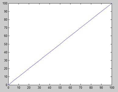
Давайте возьмем еще один пример для построения функции y = x 2 . В этом примере мы нарисуем два графика с одной и той же функцией, но во второй раз мы уменьшим значение приращения. Обратите внимание, что при уменьшении приращения график становится более плавным.
Создайте файл сценария и введите следующий код –
x = [1 2 3 4 5 6 7 8 9 10];
x = [-100:20:100];
y = x.^2;
plot(x, y)
Когда вы запускаете файл, MATLAB отображает следующий график –

Немного измените файл кода, уменьшите приращение до 5 –
x = [-100:5:100];
y = x.^2;
plot(x, y)
MATLAB рисует более плавный график –
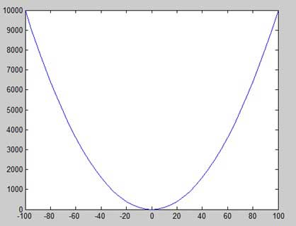
Добавление заголовка, меток, линий сетки и масштабирования на графике
MATLAB позволяет добавлять заголовки, метки вдоль осей X и Y, линии сетки, а также настраивать оси для улучшения графика.
-
Команды xlabel и ylabel генерируют метки вдоль оси x и оси y.
-
Команда title позволяет вам разместить заголовок на графике.
-
Команда grid on позволяет вам разместить линии сетки на графике.
-
Команда осевого равенства позволяет создать график с одинаковыми масштабными коэффициентами и пробелами на обеих осях.
-
Команда оси квадрат создает квадратный график.
Команды xlabel и ylabel генерируют метки вдоль оси x и оси y.
Команда title позволяет вам разместить заголовок на графике.
Команда grid on позволяет вам разместить линии сетки на графике.
Команда осевого равенства позволяет создать график с одинаковыми масштабными коэффициентами и пробелами на обеих осях.
Команда оси квадрат создает квадратный график.
пример
Создайте файл сценария и введите следующий код –
x = [0:0.01:10];
y = sin(x);
plot(x, y), xlabel('x'), ylabel('Sin(x)'), title('Sin(x) Graph'),
grid on, axis equal
MATLAB создает следующий график –

Рисование нескольких функций на одном графике
Вы можете нарисовать несколько графиков на одном графике. Следующий пример демонстрирует концепцию –
пример
Создайте файл сценария и введите следующий код –
x = [0 : 0.01: 10];
y = sin(x);
g = cos(x);
plot(x, y, x, g, '.-'), legend('Sin(x)', 'Cos(x)')
MATLAB создает следующий график –

Установка цветов на графике
MATLAB предоставляет восемь основных вариантов цвета для рисования графиков. В следующей таблице приведены цвета и их коды –
| Код | цвет |
|---|---|
| вес | белый |
| К | черный |
| б | синий |
| р | красный |
| с | Cyan |
| г | зеленый |
| м | фуксин |
| Y | желтый |
пример
Нарисуем график двух полиномов
-
f (x) = 3x 4 + 2x 3 + 7x 2 + 2x + 9 и
-
г (х) = 5х 3 + 9х + 2
f (x) = 3x 4 + 2x 3 + 7x 2 + 2x + 9 и
г (х) = 5х 3 + 9х + 2
Создайте файл сценария и введите следующий код –
x = [-10 : 0.01: 10];
y = 3*x.^4 + 2 * x.^3 + 7 * x.^2 + 2 * x + 9;
g = 5 * x.^3 + 9 * x + 2;
plot(x, y, 'r', x, g, 'g')
Когда вы запускаете файл, MATLAB генерирует следующий график –
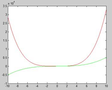
Настройка весов оси
Команда оси позволяет вам установить масштаб оси. Вы можете указать минимальное и максимальное значения для осей x и y, используя команду оси следующим образом:
axis ( [xmin xmax ymin ymax] )
Следующий пример показывает это –
пример
Создайте файл сценария и введите следующий код –
x = [0 : 0.01: 10];
y = exp(-x).* sin(2*x + 3);
plot(x, y), axis([0 10 -1 1])
Когда вы запускаете файл, MATLAB генерирует следующий график –
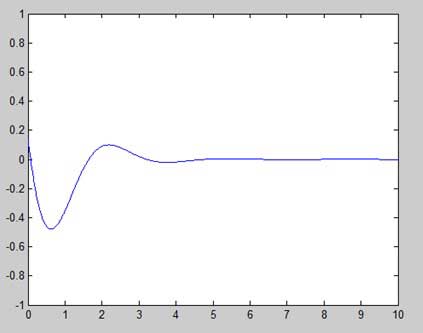
Генерация подзаговоров
Когда вы создаете массив графиков на одном и том же рисунке, каждый из этих графиков называется вложенным графиком. Команда subplot используется для создания подзаговоров.
Синтаксис для команды –
subplot(m, n, p)
где, m и n – количество строк и столбцов массива графика, а p указывает, куда поместить конкретный график.
Каждый график, созданный командой subplot, может иметь свои характеристики. Следующий пример демонстрирует концепцию –
пример
Давайте создадим два участка –
у = е -1,5х грех (10х)
у = е- 2х грех (10х)
Создайте файл сценария и введите следующий код –
x = [0:0.01:5];
y = exp(-1.5*x).*sin(10*x);
subplot(1,2,1)
plot(x,y), xlabel('x'),ylabel('exp(–1.5x)*sin(10x)'),axis([0 5 -1 1])
y = exp(-2*x).*sin(10*x);
subplot(1,2,2)
plot(x,y),xlabel('x'),ylabel('exp(–2x)*sin(10x)'),axis([0 5 -1 1])
Когда вы запускаете файл, MATLAB генерирует следующий график –

MATLAB – Графика
В этой главе мы продолжим изучение графических и графических возможностей MATLAB. Мы обсудим –
- Рисование гистограмм
- Рисование контуров
- Трехмерные участки
Рисование гистограмм
Команда bar рисует двухмерную гистограмму. Давайте возьмем пример, чтобы продемонстрировать идею.
пример
Пусть у нас будет воображаемый класс с 10 учениками. Мы знаем, что процент оценок, полученных этими студентами, составляет 75, 58, 90, 87, 50, 85, 92, 75, 60 и 95. Мы нарисуем гистограмму для этих данных.
Создайте файл сценария и введите следующий код –
x = [1:10];
y = [75, 58, 90, 87, 50, 85, 92, 75, 60, 95];
bar(x,y), xlabel('Student'),ylabel('Score'),
title('First Sem:')
print -deps graph.eps
Когда вы запускаете файл, MATLAB отображает следующую гистограмму –
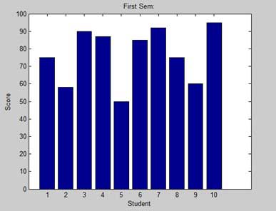
Рисование контуров
Линия контура функции двух переменных – это кривая, вдоль которой функция имеет постоянное значение. Контурные линии используются для создания контурных карт путем объединения точек равной высоты над данным уровнем, например среднего уровня моря.
MATLAB предоставляет функцию контура для рисования контурных карт.
пример
Создадим контурную карту, которая показывает контурные линии для данной функции g = f (x, y). Эта функция имеет две переменные. Итак, нам нужно будет сгенерировать две независимые переменные, то есть два набора данных x и y. Это делается путем вызова команды meshgrid .
Команда meshgrid используется для генерации матрицы элементов, которые задают диапазон по x и y, а также задают приращение в каждом случае.
Построим нашу функцию g = f (x, y), где −5 ≤ x ≤ 5, −3 ≤ y ≤ 3. Давайте возьмем приращение 0,1 для обоих значений. Переменные установлены как –
[x,y] = meshgrid(–5:0.1:5, –3:0.1:3);
Наконец, нам нужно назначить функцию. Пусть наша функция будет: x 2 + y 2
Создайте файл сценария и введите следующий код –
[x,y] = meshgrid(-5:0.1:5,-3:0.1:3);   %independent variables
g = x.^2 + y.^2;                       % our function
contour(x,y,g)                         % call the contour function
print -deps graph.eps
Когда вы запускаете файл, MATLAB отображает следующую контурную карту –

Давайте немного изменим код, чтобы украсить карту
[x,y] = meshgrid(-5:0.1:5,-3:0.1:3);   %independent variables
g = x.^2 + y.^2;                       % our function
[C, h] = contour(x,y,g);               % call the contour function
set(h,'ShowText','on','TextStep',get(h,'LevelStep')*2)
print -deps graph.eps
Когда вы запускаете файл, MATLAB отображает следующую контурную карту –
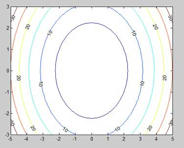
Трехмерные участки
Трехмерные графики в основном отображают поверхность, определенную функцией от двух переменных, g = f (x, y).
Как и прежде, чтобы определить g, мы сначала создаем набор точек (x, y) над областью функции, используя команду meshgrid . Далее мы назначаем саму функцию. Наконец, мы используем команду прибоя для создания графика поверхности.
Следующий пример демонстрирует концепцию –
пример
Давайте создадим трехмерную карту поверхности для функции g = xe – (x 2 + y 2 )
Создайте файл сценария и введите следующий код –
[x,y] = meshgrid(-2:.2:2);
g = x .* exp(-x.^2 - y.^2);
surf(x, y, g)
print -deps graph.eps
Когда вы запускаете файл, MATLAB отображает следующую трехмерную карту –
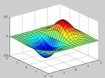
Вы также можете использовать команду сетки для создания трехмерной поверхности. Однако команда surf отображает как соединительные линии, так и грани поверхности в цвете, тогда как команда mesh создает поверхность каркаса с цветными линиями, соединяющими определяющие точки.
MATLAB – алгебра
До сих пор мы видели, что все примеры работают как в MATLAB, так и в его GNU, альтернативно называемом Octave. Но для решения основных алгебраических уравнений и MATLAB, и Octave немного отличаются, поэтому мы постараемся охватить MATLAB и Octave в отдельных разделах.
Мы также обсудим факторизацию и упрощение алгебраических выражений.
Решение основных алгебраических уравнений в MATLAB
Функция решения используется для решения алгебраических уравнений. В простейшем виде функция решения принимает в качестве аргумента уравнение, заключенное в кавычки.
Например, давайте решим для х в уравнении х-5 = 0
solve('x-5=0')
MATLAB выполнит приведенный выше оператор и вернет следующий результат –
ans =
   5
Вы также можете вызвать функцию решения как –
y = solve('x-5 = 0')
MATLAB выполнит приведенный выше оператор и вернет следующий результат –
y =
   5
Вы можете даже не включать правую часть уравнения –
solve('x-5')
MATLAB выполнит приведенный выше оператор и вернет следующий результат –
ans =
   5
Если в уравнение входит несколько символов, то по умолчанию MATLAB предполагает, что вы решаете для x, однако функция решения имеет другую форму –
solve(equation, variable)
где вы также можете упомянуть переменную.
Например, давайте решим уравнение v – u – 3t 2 = 0, для v. В этом случае мы должны написать –
solve('v-u-3*t^2=0', 'v')
MATLAB выполнит приведенный выше оператор и вернет следующий результат –
ans =
   3*t^2 + u
Решение основных алгебраических уравнений в октаве
Функция корней используется для решения алгебраических уравнений в Octave, и вы можете написать приведенные выше примеры следующим образом:
Например, давайте решим для х в уравнении х-5 = 0
Live Demo
roots([1, -5])
Octave выполнит приведенный выше оператор и вернет следующий результат –
ans = 5
Вы также можете вызвать функцию решения как –
Live Demo
y = roots([1, -5])
Octave выполнит приведенный выше оператор и вернет следующий результат –
y = 5
Решение квадратичных уравнений в MATLAB
Функция решения также может решать уравнения более высокого порядка. Он часто используется для решения квадратных уравнений. Функция возвращает корни уравнения в массиве.
В следующем примере решается квадратное уравнение x 2 -7x +12 = 0. Создайте файл сценария и введите следующий код –
eq = 'x^2 -7*x + 12 = 0';
s = solve(eq);
disp('The first root is: '), disp(s(1));
disp('The second root is: '), disp(s(2));
Когда вы запускаете файл, он показывает следующий результат –
The first root is:
   3
The second root is:
   4
Решение квадратичных уравнений в октаве
В следующем примере решается квадратное уравнение x 2 -7x +12 = 0 в октаве. Создайте файл сценария и введите следующий код –
Live Demo
s = roots([1, -7, 12]);

disp('The first root is: '), disp(s(1));
disp('The second root is: '), disp(s(2));
Когда вы запускаете файл, он показывает следующий результат –
The first root is:
   4
The second root is:
   3
Решение уравнений высшего порядка в MATLAB
Функция решения также может решать уравнения более высокого порядка. Например, давайте решим кубическое уравнение как (x-3) 2 (x-7) = 0
solve('(x-3)^2*(x-7)=0')
MATLAB выполнит приведенный выше оператор и вернет следующий результат –
ans =
   3
   3
   7
В случае уравнений более высокого порядка корни длинные, содержащие много членов. Вы можете получить числовое значение таких корней, преобразовав их в двойные. В следующем примере решается уравнение четвертого порядка x 4 – 7x 3 + 3x 2 – 5x + 9 = 0.
Создайте файл сценария и введите следующий код –
eq = 'x^4 - 7*x^3 + 3*x^2 - 5*x + 9 = 0';
s = solve(eq);
disp('The first root is: '), disp(s(1));
disp('The second root is: '), disp(s(2));
disp('The third root is: '), disp(s(3));
disp('The fourth root is: '), disp(s(4));

% converting the roots to double type
disp('Numeric value of first root'), disp(double(s(1)));
disp('Numeric value of second root'), disp(double(s(2)));
disp('Numeric value of third root'), disp(double(s(3)));
disp('Numeric value of fourth root'), disp(double(s(4)));
Когда вы запускаете файл, он возвращает следующий результат –
The first root is:
6.630396332390718431485053218985
 The second root is:
1.0597804633025896291682772499885
 The third root is:
- 0.34508839784665403032666523448675 - 1.0778362954630176596831109269793*i
 The fourth root is:
- 0.34508839784665403032666523448675 + 1.0778362954630176596831109269793*i
Numeric value of first root
   6.6304
Numeric value of second root
   1.0598
Numeric value of third root
   -0.3451 - 1.0778i
Numeric value of fourth root
   -0.3451 + 1.0778i
Обратите внимание, что последние два корня являются комплексными числами.
Решение уравнений высшего порядка в октаве
В следующем примере решается уравнение четвертого порядка x 4 – 7x 3 + 3x 2 – 5x + 9 = 0.
Создайте файл сценария и введите следующий код –
Live Demo
v = [1, -7,  3, -5, 9];
s = roots(v);

% converting the roots to double type
disp('Numeric value of first root'), disp(double(s(1)));
disp('Numeric value of second root'), disp(double(s(2)));
disp('Numeric value of third root'), disp(double(s(3)));
disp('Numeric value of fourth root'), disp(double(s(4)));
Когда вы запускаете файл, он возвращает следующий результат –
Numeric value of first root
 6.6304
Numeric value of second root
-0.34509 + 1.07784i
Numeric value of third root
-0.34509 - 1.07784i
Numeric value of fourth root
 1.0598
Решение системы уравнений в MATLAB
Функция решения также может быть использована для генерации решений систем уравнений, включающих более одной переменной. Давайте рассмотрим простой пример, чтобы продемонстрировать это использование.
Давайте решим уравнения –
5x + 9y = 5
3x – 6y = 4
Создайте файл сценария и введите следующий код –
s = solve('5*x + 9*y = 5','3*x - 6*y = 4');
s.x
s.y
Когда вы запускаете файл, он показывает следующий результат –
ans =
   22/19
ans =
   -5/57
Таким же образом вы можете решать большие линейные системы. Рассмотрим следующую систему уравнений –
х + 3й -2z = 5
3x + 5y + 6z = 7
2x + 4y + 3z = 8
Решающая система уравнений в октаве
У нас есть немного другой подход к решению системы ‘n’ линейных уравнений с ‘n’ неизвестными. Давайте рассмотрим простой пример, чтобы продемонстрировать это использование.
Давайте решим уравнения –
5x + 9y = 5
3x – 6y = 4
Такая система линейных уравнений может быть записана в виде единого матричного уравнения Ax = b, где A – матрица коэффициентов, b – вектор столбцов, содержащий правую часть линейных уравнений, а x – вектор столбцов, представляющий решение как показано в программе ниже –
Создайте файл сценария и введите следующий код –
Live Demo
A = [5, 9; 3, -6];
b = [5;4];
A  b
Когда вы запускаете файл, он показывает следующий результат –
ans =

   1.157895
  -0.087719
Таким же образом, вы можете решить большие линейные системы, как указано ниже –
х + 3й -2z = 5
3x + 5y + 6z = 7
2x + 4y + 3z = 8
Разложение и сбор уравнений в MATLAB
Функция расширения и сбора расширяет и собирает уравнение соответственно. Следующий пример демонстрирует понятия –
Когда вы работаете со многими символическими функциями, вы должны объявить, что ваши переменные являются символическими.
Создайте файл сценария и введите следующий код –
syms x   %symbolic variable x
syms y   %symbolic variable x
% expanding equations
expand((x-5)*(x+9))
expand((x+2)*(x-3)*(x-5)*(x+7))
expand(sin(2*x))
expand(cos(x+y))

% collecting equations
collect(x^3 *(x-7))
collect(x^4*(x-3)*(x-5))
Когда вы запускаете файл, он показывает следующий результат –
ans =
   x^2 + 4*x - 45
ans =
   x^4 + x^3 - 43*x^2 + 23*x + 210
ans =
   2*cos(x)*sin(x)
ans =
   cos(x)*cos(y) - sin(x)*sin(y)
ans =
   x^4 - 7*x^3
ans =
   x^6 - 8*x^5 + 15*x^4
Расширяя и собирая уравнения в октаве
Вам нужно иметь символьный пакет, который обеспечивает расширение и функцию сбора для расширения и сбора уравнения, соответственно. Следующий пример демонстрирует понятия –
Когда вы работаете со многими символическими функциями, вы должны объявить, что ваши переменные являются символическими, но у Octave другой подход к определению символических переменных. Обратите внимание на использование Sin и Cos , которые также определены в символической упаковке.
Создайте файл сценария и введите следующий код –
% first of all load the package, make sure its installed.
pkg load symbolic

% make symbols module available
symbols

% define symbolic variables
x = sym ('x');
y = sym ('y');
z = sym ('z');

% expanding equations
expand((x-5)*(x+9))
expand((x+2)*(x-3)*(x-5)*(x+7))
expand(Sin(2*x))
expand(Cos(x+y))

% collecting equations
collect(x^3 *(x-7), z)
collect(x^4*(x-3)*(x-5), z)
Когда вы запускаете файл, он показывает следующий результат –
ans =

-45.0+x^2+(4.0)*x
ans =

210.0+x^4-(43.0)*x^2+x^3+(23.0)*x
ans =

sin((2.0)*x)
ans =

cos(y+x)
ans =

x^(3.0)*(-7.0+x)
ans =

(-3.0+x)*x^(4.0)*(-5.0+x)
Факторизация и упрощение алгебраических выражений
Факторная функция разлагает выражение, а функция упрощения упрощает выражение. Следующий пример демонстрирует концепцию –
пример
Создайте файл сценария и введите следующий код –
syms x
syms y
factor(x^3 - y^3)
factor([x^2-y^2,x^3+y^3])
simplify((x^4-16)/(x^2-4))
Когда вы запускаете файл, он показывает следующий результат –
ans =
   (x - y)*(x^2 + x*y + y^2)
ans =
   [ (x - y)*(x + y), (x + y)*(x^2 - x*y + y^2)]
ans =
   x^2 + 4
MATLAB – Исчисление
MATLAB предоставляет различные способы решения задач дифференциального и интегрального исчисления, решения дифференциальных уравнений любой степени и расчета пределов. Лучше всего, вы можете легко построить графики сложных функций и проверить максимумы, минимумы и другие точки канцелярских товаров на графике, решив исходную функцию, а также ее производную.
В этой главе будут рассмотрены проблемы исчисления. В этой главе мы обсудим концепции предисчисления, то есть вычисления пределов функций и проверки свойств пределов.
В следующей главе Дифференциал мы вычислим производную выражения и найдем локальные максимумы и минимумы на графе. Мы также обсудим решение дифференциальных уравнений.
Наконец, в главе « Интеграция» мы обсудим интегральное исчисление.
Расчет лимитов
MATLAB предоставляет функцию предела для расчета пределов. В своей основной форме функция limit принимает выражение в качестве аргумента и находит предел выражения, когда независимая переменная стремится к нулю.
Например, давайте вычислим предел функции f (x) = (x 3 + 5) / (x 4 + 7), когда x стремится к нулю.
syms x
limit((x^3 + 5)/(x^4 + 7))
MATLAB выполнит приведенный выше оператор и вернет следующий результат –
ans =
   5/7
Функция предела относится к области символьных вычислений; вам нужно использовать функцию syms, чтобы сообщить MATLAB, какие символические переменные вы используете. Вы также можете вычислить предел функции, так как переменная стремится к некоторому числу, отличному от нуля. Чтобы вычислить lim x-> a (f (x)), мы используем команду limit с аргументами. Первое – это выражение, а второе – число, к которому подходит x , здесь это a .
Например, давайте вычислим предел функции f (x) = (x-3) / (x-1), поскольку x стремится к 1.
limit((x - 3)/(x-1),1)
MATLAB выполнит приведенный выше оператор и вернет следующий результат –
ans =
   NaN
Давайте возьмем другой пример,
limit(x^2 + 5, 3)
MATLAB выполнит приведенный выше оператор и вернет следующий результат –
ans =
   14
Расчет лимитов с использованием октавы
Ниже приведена октавная версия приведенного выше примера с использованием символического пакета, попробуйте выполнить и сравнить результат –
pkg load symbolic
symbols

x = sym("x");
subs((x^3+5)/(x^4+7),x,0)
Octave выполнит приведенный выше оператор и вернет следующий результат –
ans =
   0.7142857142857142857
Проверка основных свойств пределов
Алгебраическая предельная теорема обеспечивает некоторые основные свойства пределов. Это следующие –

Давайте рассмотрим две функции –
- f (x) = (3x + 5) / (x – 3)
- г (х) = х 2 + 1.
Давайте вычислим пределы функций при стремлении x к 5 для обеих функций и проверим основные свойства пределов, используя эти две функции и MATLAB.
пример
Создайте файл сценария и введите в него следующий код –
syms x
f = (3*x + 5)/(x-3);
g = x^2 + 1;
l1 = limit(f, 4)
l2 = limit (g, 4)
lAdd = limit(f + g, 4)
lSub = limit(f - g, 4)
lMult = limit(f*g, 4)
lDiv = limit (f/g, 4)
Когда вы запускаете файл, он отображает –
l1 =
   17

l2 =
   17

lAdd =
   34

lSub =
   0

lMult =
   289

lDiv =
   1
Проверка основных свойств лимитов с использованием октавы
Ниже приведена октавная версия приведенного выше примера с использованием символического пакета, попробуйте выполнить и сравнить результат –
pkg load symbolic
symbols

x = sym("x");
f = (3*x + 5)/(x-3);
g = x^2 + 1;

l1 = subs(f, x, 4)
l2 = subs (g, x, 4)
lAdd = subs (f+g, x, 4)
lSub = subs (f-g, x, 4)
lMult = subs (f*g, x, 4)
lDiv = subs (f/g, x, 4)
Octave выполнит приведенный выше оператор и вернет следующий результат –
l1 =
   17.0
l2 =
   17.0
lAdd =
   34.0
lSub =
   0.0
lMult =
   289.0
lDiv =
   1.0
Левый и Правосторонний Пределы
Когда функция имеет разрыв для некоторого конкретного значения переменной, в этой точке ограничение не существует. Другими словами, пределы функции f (x) имеют разрыв при x = a, когда значение предела, когда x приближается к x с левой стороны, не равно значению предела, когда x приближается с правой стороны.
Это приводит к концепции пределов для левшей и правшей. Предел для левой руки определяется как предел как x -> a слева, т. Е. X приближается к a для значений x <a. Правосторонний предел определяется как предел как x -> a справа, т. Е. X приближается к a для значений x> a. Когда левосторонний лимит и правосторонний лимит не равны, этот предел не существует.
Давайте рассмотрим функцию –
f (x) = (x – 3) / | x – 3 |
Покажем, что lim x-> 3 f (x) не существует. MATLAB помогает нам установить этот факт двумя способами –
- Построить график функции и показать разрыв.
- Вычисляя пределы и показывая, что оба они разные.
Пределы для левшей и правшей вычисляются путем передачи строк символов ‘left’ и ‘right’ в команду limit в качестве последнего аргумента.
пример
Создайте файл сценария и введите в него следующий код –
f = (x - 3)/abs(x-3);
ezplot(f,[-1,5])
l = limit(f,x,3,'left')
r = limit(f,x,3,'right')
Когда вы запускаете файл, MATLAB рисует следующий график
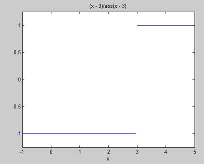
После этого отображается следующий вывод –
l =
   -1

r =
   1
MATLAB – Дифференциал
MATLAB предоставляет команду diff для вычисления символьных производных. В простейшей форме вы передаете функцию, которую вы хотите дифференцировать, команде diff в качестве аргумента.
Например, давайте вычислим производную функции f (t) = 3t 2 + 2t -2
пример
Создайте файл сценария и введите в него следующий код –
syms t
f = 3*t^2 + 2*t^(-2);
diff(f)
Когда приведенный выше код компилируется и выполняется, он дает следующий результат –
ans =
6*t - 4/t^3
Ниже приведен октавный эквивалент приведенного выше расчета –
pkg load symbolic
symbols

t = sym("t");
f = 3*t^2 + 2*t^(-2);
differentiate(f,t)
Octave выполняет код и возвращает следующий результат –
ans =
   -(4.0)*t^(-3.0)+(6.0)*t
Проверка элементарных правил дифференциации
Кратко сформулируем различные уравнения или правила дифференцирования функций и проверим эти правила. Для этого мы напишем f ‘(x) для производной первого порядка и f “(x) для производной второго порядка.
Ниже приведены правила для дифференциации –
Правило 1
Для любых функций f и g и любых действительных чисел a и b являются производными функции –
h (x) = af (x) + bg (x) относительно x определяется как –
h ‘(x) = af’ (x) + bg ‘(x)
Правило 2
Правила сумм и вычитаний гласят, что если f и g две функции, то f ‘и g’ являются их производными соответственно, тогда
( f + g) ‘= f’ + g ‘
(f – g) ‘= f’ – g ‘
Правило 3
Правило произведения гласит, что если f и g две функции, f ‘и g’ являются их производными соответственно, то
(fg) ‘= f’.g + g’.f
Правило 4
Правило отношения гласит, что если f и g две функции, f ‘и g’ являются их производными соответственно, то
(f / g) ‘= (f’.g – g’.f) / g 2
Правило 5
Полиномиальное или элементарное степенное правило гласит, что если y = f (x) = x n , то f ‘= n. х (н-1)
Прямым результатом этого правила является то, что производная любой константы равна нулю, т. Е. Если y = k , любая константа, то
f ‘= 0
Правило 6
Правило цепочки гласит, что производная функции функции h (x) = f (g (x)) по x равна
h ‘(x) = f’ (g (x)). g ‘(x)
пример
Создайте файл сценария и введите в него следующий код –
syms x
syms t

f = (x + 2)*(x^2 + 3)
der1 = diff(f)
f = (t^2 + 3)*(sqrt(t) + t^3)
der2 = diff(f)
f = (x^2 - 2*x + 1)*(3*x^3 - 5*x^2 + 2)
der3 = diff(f)
f = (2*x^2 + 3*x)/(x^3 + 1)
der4 = diff(f)
f = (x^2 + 1)^17
der5 = diff(f)
f = (t^3 + 3* t^2 + 5*t -9)^(-6)
der6 = diff(f)
Когда вы запускаете файл, MATLAB отображает следующий результат –
f =
   (x^2 + 3)*(x + 2)

   der1 =
   2*x*(x + 2) + x^2 + 3

f =
   (t^(1/2) + t^3)*(t^2 + 3)

   der2 =
   (t^2 + 3)*(3*t^2 + 1/(2*t^(1/2))) + 2*t*(t^(1/2) + t^3)

f =
   (x^2 - 2*x + 1)*(3*x^3 - 5*x^2 + 2)

der3 =
   (2*x - 2)*(3*x^3 - 5*x^2 + 2) - (- 9*x^2 + 10*x)*(x^2 - 2*x + 1)

f =
   (2*x^2 + 3*x)/(x^3 + 1)

der4 =
   (4*x + 3)/(x^3 + 1) - (3*x^2*(2*x^2 + 3*x))/(x^3 + 1)^2

f =
   (x^2 + 1)^17

der5 =
   34*x*(x^2 + 1)^16

f =
   1/(t^3 + 3*t^2 + 5*t - 9)^6

der6 =
   -(6*(3*t^2 + 6*t + 5))/(t^3 + 3*t^2 + 5*t - 9)^7
Ниже приведен октавный эквивалент приведенного выше расчета –
pkg load symbolic
symbols

x = sym("x");
t = sym("t");
f = (x + 2)*(x^2 + 3)
der1 = differentiate(f,x)
f = (t^2 + 3)*(t^(1/2) + t^3)
der2 = differentiate(f,t)
f = (x^2 - 2*x + 1)*(3*x^3 - 5*x^2 + 2)
der3 = differentiate(f,x)
f = (2*x^2 + 3*x)/(x^3 + 1)
der4 = differentiate(f,x)
f = (x^2 + 1)^17
der5 = differentiate(f,x)
f = (t^3 + 3* t^2 + 5*t -9)^(-6)
der6 = differentiate(f,t)
Octave выполняет код и возвращает следующий результат –
f =

(2.0+x)*(3.0+x^(2.0))
der1 =

3.0+x^(2.0)+(2.0)*(2.0+x)*x
f =

(t^(3.0)+sqrt(t))*(3.0+t^(2.0))
der2 =

(2.0)*(t^(3.0)+sqrt(t))*t+((3.0)*t^(2.0)+(0.5)*t^(-0.5))*(3.0+t^(2.0))
f =

(1.0+x^(2.0)-(2.0)*x)*(2.0-(5.0)*x^(2.0)+(3.0)*x^(3.0))
der3 =

(-2.0+(2.0)*x)*(2.0-(5.0)*x^(2.0)+(3.0)*x^(3.0))+((9.0)*x^(2.0)-(10.0)*x)*(1.0+x^(2.0)-(2.0)*x)
f =

(1.0+x^(3.0))^(-1)*((2.0)*x^(2.0)+(3.0)*x)
der4 =

(1.0+x^(3.0))^(-1)*(3.0+(4.0)*x)-(3.0)*(1.0+x^(3.0))^(-2)*x^(2.0)*((2.0)*x^(2.0)+(3.0)*x)
f =

(1.0+x^(2.0))^(17.0)
der5 =

(34.0)*(1.0+x^(2.0))^(16.0)*x
f =

(-9.0+(3.0)*t^(2.0)+t^(3.0)+(5.0)*t)^(-6.0)
der6 =

-(6.0)*(-9.0+(3.0)*t^(2.0)+t^(3.0)+(5.0)*t)^(-7.0)*(5.0+(3.0)*t^(2.0)+(6.0)*t)
Производные экспоненциальных, логарифмических и тригонометрических функций
В следующей таблице приведены производные от часто используемых экспоненциальных, логарифмических и тригонометрических функций.
| функция | производный |
|---|---|
| топор с | c ax. ln ca (ln – натуральный логарифм) |
| е х | е х |
| ln x | 1 / х |
| ln c x | 1 / x.ln c |
| х х | х х (1 + лн х) |
| грех (х) | сов (х) |
| сов (х) | -sin (х) |
| тангенс (х) | sec 2 (x), или 1 / cos 2 (x), или 1 + tan 2 (x) |
| кроватка (х) | -csc 2 (x) или -1 / sin 2 (x) или – (1 + кроватка 2 (x)) |
| с (х) | с (х) .tan (х) |
| CSC (х) | -csc (х) .cot (х) |
пример
Создайте файл сценария и введите в него следующий код –
syms x
y = exp(x)
diff(y)
y = x^9
diff(y)
y = sin(x)
diff(y)
y = tan(x)
diff(y)
y = cos(x)
diff(y)
y = log(x)
diff(y)
y = log10(x)
diff(y)
y = sin(x)^2
diff(y)
y = cos(3*x^2 + 2*x + 1)
diff(y)
y = exp(x)/sin(x)
diff(y)
Когда вы запускаете файл, MATLAB отображает следующий результат –
y =
   exp(x)
   ans =
   exp(x)

y =
   x^9
   ans =
   9*x^8

y =
   sin(x)
   ans =
   cos(x)

y =
   tan(x)
   ans =
   tan(x)^2 + 1

y =
   cos(x)
   ans =
   -sin(x)

y =
   log(x)
   ans =
   1/x

y =
   log(x)/log(10)
   ans =
   1/(x*log(10))

y =
   sin(x)^2
   ans =
   2*cos(x)*sin(x)

y =
   cos(3*x^2 + 2*x + 1)
   ans =
   -sin(3*x^2 + 2*x + 1)*(6*x + 2)

y =
   exp(x)/sin(x)
   ans =
   exp(x)/sin(x) - (exp(x)*cos(x))/sin(x)^2
Ниже приведен октавный эквивалент приведенного выше расчета –
pkg load symbolic
symbols

x = sym("x");
y = Exp(x)
differentiate(y,x)

y = x^9
differentiate(y,x)

y = Sin(x)
differentiate(y,x)

y = Tan(x)
differentiate(y,x)

y = Cos(x)
differentiate(y,x)

y = Log(x)
differentiate(y,x)

% symbolic packages does not have this support
%y = Log10(x)
%differentiate(y,x)

y = Sin(x)^2
differentiate(y,x)

y = Cos(3*x^2 + 2*x + 1)
differentiate(y,x)

y = Exp(x)/Sin(x)
differentiate(y,x)
Octave выполняет код и возвращает следующий результат –
y =

exp(x)
ans =

exp(x)
y =

x^(9.0)
ans =

(9.0)*x^(8.0)
y =

sin(x)
ans =

cos(x)
y =

tan(x)
ans =

1+tan(x)^2
y =

cos(x)
ans =

-sin(x)
y =

log(x)
ans =

x^(-1)
y =

sin(x)^(2.0)
ans =

(2.0)*sin(x)*cos(x)
y =

cos(1.0+(2.0)*x+(3.0)*x^(2.0))
ans =

-(2.0+(6.0)*x)*sin(1.0+(2.0)*x+(3.0)*x^(2.0))
y =

sin(x)^(-1)*exp(x)
ans =

sin(x)^(-1)*exp(x)-sin(x)^(-2)*cos(x)*exp(x)
Вычисление производных высшего порядка
Для вычисления старших производных функции f мы используем синтаксис diff (f, n) .
Вычислим вторую производную функции y = f (x) = x .e -3x
f = x*exp(-3*x);
diff(f, 2)
MATLAB выполняет код и возвращает следующий результат –
ans =
9*x*exp(-3*x) - 6*exp(-3*x)
Ниже приведен октавный эквивалент приведенного выше расчета –
pkg load symbolic
symbols

x = sym("x");
f = x*Exp(-3*x);
differentiate(f, x, 2)
Octave выполняет код и возвращает следующий результат –
ans =

(9.0)*exp(-(3.0)*x)*x-(6.0)*exp(-(3.0)*x)
пример
В этом примере давайте решим проблему. Учитывая, что функция y = f (x) = 3 sin (x) + 7 cos (5x) . Нам нужно выяснить, выполняется ли уравнение f “+ f = -5cos (2x) .
Создайте файл сценария и введите в него следующий код –
syms x
y = 3*sin(x)+7*cos(5*x);  % defining the function
lhs = diff(y,2)+y;        %evaluting the lhs of the equation
rhs = -5*cos(2*x);        %rhs of the equation
if(isequal(lhs,rhs))
   disp('Yes, the equation holds true');
else
   disp('No, the equation does not hold true');
end
disp('Value of LHS is: '), disp(lhs);
Когда вы запускаете файл, он показывает следующий результат –
No, the equation does not hold true
Value of LHS is:
-168*cos(5*x)
Ниже приведен октавный эквивалент приведенного выше расчета –
pkg load symbolic
symbols

x = sym("x");
y = 3*Sin(x)+7*Cos(5*x);           % defining the function
lhs = differentiate(y, x, 2) + y;  %evaluting the lhs of the equation
rhs = -5*Cos(2*x);                 %rhs of the equation

if(lhs == rhs)
   disp('Yes, the equation holds true');
else
   disp('No, the equation does not hold true');
end
disp('Value of LHS is: '), disp(lhs);
Octave выполняет код и возвращает следующий результат –
No, the equation does not hold true
Value of LHS is:
-(168.0)*cos((5.0)*x)
Нахождение максимумов и минимумов кривой
Если мы ищем локальные максимумы и минимумы для графика, мы в основном ищем самые высокие или самые низкие точки на графике функции в определенной местности или для определенного диапазона значений символической переменной.
Для функции y = f (x) точки на графе, где граф имеет нулевой наклон, называются стационарными точками . Другими словами, стационарные точки – это где f ‘(x) = 0.
Чтобы найти стационарные точки функции, которую мы дифференцируем, нам нужно установить производную равной нулю и решить уравнение.
пример
Найдем стационарные точки функции f (x) = 2x 3 + 3x 2 – 12x + 17
Сделайте следующие шаги –
Сначала давайте введем функцию и построим ее график.
syms x
y = 2*x^3 + 3*x^2 - 12*x + 17;   % defining the function
ezplot(y)
MATLAB выполняет код и возвращает следующий график –

Вот октавный эквивалентный код для приведенного выше примера –
pkg load symbolic
symbols

x = sym('x');
y = inline("2*x^3 + 3*x^2 - 12*x + 17");

ezplot(y)
print -deps graph.eps
Наша цель – найти некоторые локальные максимумы и минимумы на графике, поэтому давайте найдем локальные максимумы и минимумы для интервала [-2, 2] на графике.
syms x
y = 2*x^3 + 3*x^2 - 12*x + 17;   % defining the function
ezplot(y, [-2, 2])
MATLAB выполняет код и возвращает следующий график –
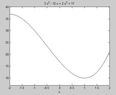
Вот октавный эквивалентный код для приведенного выше примера –
pkg load symbolic
symbols

x = sym('x');
y = inline("2*x^3 + 3*x^2 - 12*x + 17");

ezplot(y, [-2, 2])
print -deps graph.eps
Далее, давайте вычислим производную.
g = diff(y)
MATLAB выполняет код и возвращает следующий результат –
g = 6*x^2 + 6*x - 12
Вот октавный эквивалент приведенного выше расчета –
pkg load symbolic symbols x = sym("x"); y = 2*x^3 + 3*x^2 - 12*x + 17; g = differentiate(y,x)
Octave выполняет код и возвращает следующий результат –
g = -12.0+(6.0)*x+(6.0)*x^(2.0)
Давайте решим производную функцию g, чтобы получить значения, где она становится равной нулю.
s = solve(g)
MATLAB выполняет код и возвращает следующий результат –
s = 1 -2
Ниже приведен октавный эквивалент приведенного выше расчета –
pkg load symbolic symbols x = sym("x"); y = 2*x^3 + 3*x^2 - 12*x + 17; g = differentiate(y,x) roots([6, 6, -12])
Octave выполняет код и возвращает следующий результат –
g = -12.0+(6.0)*x^(2.0)+(6.0)*x ans = -2 1
Это согласуется с нашим сюжетом. Итак, давайте оценим функцию f в критических точках x = 1, -2. Мы можем подставить значение в символическую функцию с помощью команды subs .
subs(y, 1), subs(y, -2)
MATLAB выполняет код и возвращает следующий результат –
ans = 10 ans = 37
Ниже приведен октавный эквивалент приведенного выше расчета –
pkg load symbolic symbols x = sym("x"); y = 2*x^3 + 3*x^2 - 12*x + 17; g = differentiate(y,x) roots([6, 6, -12]) subs(y, x, 1), subs(y, x, -2)
ans = 10.0 ans = 37.0-4.6734207789940138748E-18*I
Следовательно, минимальное и максимальное значения для функции f (x) = 2x 3 + 3x 2 – 12x + 17 в интервале [-2,2] составляют 10 и 37.
Решение дифференциальных уравнений
MATLAB предоставляет команду dsolve для символического решения дифференциальных уравнений.
Наиболее простой формой команды dsolve для поиска решения одного уравнения является
dsolve('eqn')
где eqn – текстовая строка, используемая для ввода уравнения.
Он возвращает символическое решение с набором произвольных констант, которые MATLAB помечает C1, C2 и так далее.
Вы также можете указать начальные и граничные условия для задачи в виде списка с разделителями-запятыми после уравнения в виде –
dsolve('eqn','cond1', 'cond2',…)
В целях использования команды dsolve производные обозначены знаком D. Например, уравнение типа f ‘(t) = -2 * f + стоимость (t) вводится как –
‘Df = -2 * f + cos (t)’
Высшие производные обозначены следующим за D порядком производной.
Например, уравнение f “(x) + 2f ‘(x) = 5sin3x должно быть введено как –
‘D2y + 2Dy = 5 * sin (3 * x)’
Давайте рассмотрим простой пример дифференциального уравнения первого порядка: y ‘= 5y.
s = dsolve('Dy = 5*y')
MATLAB выполняет код и возвращает следующий результат –
s = C2*exp(5*t)
Давайте рассмотрим другой пример дифференциального уравнения второго порядка: y “- y = 0, y (0) = -1, y ‘(0) = 2.
dsolve('D2y - y = 0','y(0) = -1','Dy(0) = 2')
MATLAB выполняет код и возвращает следующий результат –
ans = exp(t)/2 - (3*exp(-t))/2
MATLAB – Интеграция
Интеграция имеет дело с двумя принципиально разными типами проблем.
-
В первом типе дается производная функции, и мы хотим найти функцию. Поэтому мы в основном обращаем вспять процесс дифференциации. Этот обратный процесс известен как антидифференцирование, или нахождение примитивной функции, или нахождение неопределенного интеграла .
-
Второй тип проблем включает сложение очень большого количества очень маленьких величин, а затем определение предела, когда размер величин приближается к нулю, а число членов стремится к бесконечности. Этот процесс приводит к определению определенного интеграла .
В первом типе дается производная функции, и мы хотим найти функцию. Поэтому мы в основном обращаем вспять процесс дифференциации. Этот обратный процесс известен как антидифференцирование, или нахождение примитивной функции, или нахождение неопределенного интеграла .
Второй тип проблем включает сложение очень большого количества очень маленьких величин, а затем определение предела, когда размер величин приближается к нулю, а число членов стремится к бесконечности. Этот процесс приводит к определению определенного интеграла .
Определенные интегралы используются для определения площади, объема, центра тяжести, момента инерции, работы, выполняемой силой, и во многих других приложениях.
Поиск неопределенного интеграла с помощью MATLAB
По определению, если производная функции f (x) есть f ‘(x), то мы говорим, что неопределенный интеграл от f’ (x) по x равен f (x). Например, поскольку производная (по x) x 2 равна 2x, мы можем сказать, что неопределенный интеграл от 2x равен x 2 .
В символах –
f ‘(x 2 ) = 2x , следовательно,
∫ 2xdx = x 2 .
Неопределенный интеграл не является уникальным, потому что производная x 2 + c для любого значения константы c также будет 2x.
Это выражается в символах как –
∫ 2xdx = x 2 + c .
Где c называется «произвольной константой».
MATLAB предоставляет команду int для вычисления интеграла выражения. Чтобы вывести выражение для неопределенного интеграла функции, мы пишем –
int(f);
Например, из нашего предыдущего примера –
syms x int(2*x)
MATLAB выполняет приведенный выше оператор и возвращает следующий результат –
ans = x^2
Пример 1
В этом примере давайте найдем интеграл некоторых часто используемых выражений. Создайте файл сценария и введите в нем следующий код –
syms x n int(sym(x^n)) f = 'sin(n*t)' int(sym(f)) syms a t int(a*cos(pi*t)) int(a^x)
Когда вы запускаете файл, он показывает следующий результат –
ans = piecewise([n == -1, log(x)], [n ~= -1, x^(n + 1)/(n + 1)]) f = sin(n*t) ans = -cos(n*t)/n ans = (a*sin(pi*t))/pi ans = a^x/log(a)
Пример 2
Создайте файл сценария и введите в нем следующий код –
syms x n int(cos(x)) int(exp(x)) int(log(x)) int(x^-1) int(x^5*cos(5*x)) pretty(int(x^5*cos(5*x))) int(x^-5) int(sec(x)^2) pretty(int(1 - 10*x + 9 * x^2)) int((3 + 5*x -6*x^2 - 7*x^3)/2*x^2) pretty(int((3 + 5*x -6*x^2 - 7*x^3)/2*x^2))
Обратите внимание, что функция pretty возвращает выражение в более читаемом формате.
Когда вы запускаете файл, он показывает следующий результат –
ans =
sin(x)
ans =
exp(x)
ans =
x*(log(x) - 1)
ans =
log(x)
ans =
(24*cos(5*x))/3125 + (24*x*sin(5*x))/625 - (12*x^2*cos(5*x))/125 + (x^4*cos(5*x))/5 - (4*x^3*sin(5*x))/25 + (x^5*sin(5*x))/5
2 4
24 cos(5 x) 24 x sin(5 x) 12 x cos(5 x) x cos(5 x)
----------- + ------------- - -------------- + ------------
3125 625 125 5
3 5
4 x sin(5 x) x sin(5 x)
------------- + -----------
25 5
ans =
-1/(4*x^4)
ans =
tan(x)
2
x (3 x - 5 x + 1)
ans =
- (7*x^6)/12 - (3*x^5)/5 + (5*x^4)/8 + x^3/2
6 5 4 3
7 x 3 x 5 x x
- ---- - ---- + ---- + --
12 5 8 2
Нахождение определенного интеграла с помощью MATLAB
По определению, определенный интеграл в основном является пределом суммы. Мы используем определенные интегралы, чтобы найти области, такие как область между кривой и осью x и область между двумя кривыми. Определенные интегралы могут также использоваться в других ситуациях, где требуемое количество может быть выражено как предел суммы.
Функция int может использоваться для определенной интеграции, передавая пределы, по которым вы хотите вычислить интеграл.
Вычислять

мы пишем,
int(x, a, b)
Например, для расчета стоимости  мы пишем –
int(x, 4, 9)
MATLAB выполняет приведенный выше оператор и возвращает следующий результат –
ans = 65/2
Ниже приведен октавный эквивалент приведенного выше расчета –
pkg load symbolic symbols x = sym("x"); f = x; c = [1, 0]; integral = polyint(c); a = polyval(integral, 9) - polyval(integral, 4); display('Area: '), disp(double(a));
Octave выполняет код и возвращает следующий результат –
Area: 32.500
Альтернативное решение может быть дано с помощью функции quad (), предоставляемой Octave следующим образом:
pkg load symbolic symbols f = inline("x"); [a, ierror, nfneval] = quad(f, 4, 9); display('Area: '), disp(double(a));
Octave выполняет код и возвращает следующий результат –
Area: 32.500
Пример 1
Вычислим площадь, заключенную между осью x и кривой y = x 3 -2x + 5 и ординатами x = 1 и x = 2.
Требуемая площадь определяется как –

Создайте файл сценария и введите следующий код –
f = x^3 - 2*x +5; a = int(f, 1, 2) display('Area: '), disp(double(a));
Когда вы запускаете файл, он показывает следующий результат –
a = 23/4 Area: 5.7500
Ниже приведен октавный эквивалент приведенного выше расчета –
pkg load symbolic symbols x = sym("x"); f = x^3 - 2*x +5; c = [1, 0, -2, 5]; integral = polyint(c); a = polyval(integral, 2) - polyval(integral, 1); display('Area: '), disp(double(a));
Octave выполняет код и возвращает следующий результат –
Area: 5.7500
Альтернативное решение может быть дано с помощью функции quad (), предоставляемой Octave следующим образом:
pkg load symbolic symbols x = sym("x"); f = inline("x^3 - 2*x +5"); [a, ierror, nfneval] = quad(f, 1, 2); display('Area: '), disp(double(a));
Octave выполняет код и возвращает следующий результат –
Area: 5.7500
Пример 2
Найдите площадь под кривой: f (x) = x 2 cos (x) для −4 ≤ x ≤ 9.
Создайте файл сценария и напишите следующий код –
f = x^2*cos(x); ezplot(f, [-4,9]) a = int(f, -4, 9) disp('Area: '), disp(double(a));
Когда вы запускаете файл, MATLAB строит график –

Выход дан ниже –
a = 8*cos(4) + 18*cos(9) + 14*sin(4) + 79*sin(9) Area: 0.3326
Ниже приведен октавный эквивалент приведенного выше расчета –
pkg load symbolic symbols x = sym("x"); f = inline("x^2*cos(x)"); ezplot(f, [-4,9]) print -deps graph.eps [a, ierror, nfneval] = quad(f, -4, 9); display('Area: '), disp(double(a));
MATLAB – многочлены
MATLAB представляет полиномы как векторы строк, содержащие коэффициенты, упорядоченные по убыванию степеней. Например, уравнение P (x) = x 4 + 7x 3 – 5x + 9 может быть представлено как –
р = [1 7 0 -5 9];
Оценка полиномов
Функция polyval используется для оценки полинома по указанному значению. Например, чтобы оценить наш предыдущий полином p при x = 4, введите –
Live Demo
p = [1 7 0 -5 9]; polyval(p,4)
MATLAB выполняет вышеуказанные операторы и возвращает следующий результат –
ans = 693
MATLAB также предоставляет функцию поливалма для вычисления матричного полинома. Матричный полином – это полином с матрицами в качестве переменных.
Например, давайте создадим квадратную матрицу X и оценим многочлен p, в X –
Live Demo
p = [1 7 0 -5 9]; X = [1 2 -3 4; 2 -5 6 3; 3 1 0 2; 5 -7 3 8]; polyvalm(p, X)
MATLAB выполняет вышеуказанные операторы и возвращает следующий результат –
ans =
2307 -1769 -939 4499
2314 -2376 -249 4695
2256 -1892 -549 4310
4570 -4532 -1062 9269
Нахождение корней полиномов
Функция корней вычисляет корни многочлена. Например, чтобы вычислить корни нашего полинома p, наберите
Live Demo
p = [1 7 0 -5 9]; r = roots(p)
MATLAB выполняет вышеуказанные операторы и возвращает следующий результат –
r = -6.8661 + 0.0000i -1.4247 + 0.0000i 0.6454 + 0.7095i 0.6454 - 0.7095i
Функция poly является обратной функцией корней и возвращается к полиномиальным коэффициентам. Например –
p2 = poly(r)
MATLAB выполняет вышеуказанные операторы и возвращает следующий результат –
p2 =
Columns 1 through 3:
1.00000 + 0.00000i 7.00000 + 0.00000i 0.00000 + 0.00000i
Columns 4 and 5:
-5.00000 - 0.00000i 9.00000 + 0.00000i
Фитинг полиномиальной кривой
Функция polyfit находит коэффициенты полинома, который соответствует набору данных в смысле наименьших квадратов. Если x и y – это два вектора, содержащие данные x и y, которые нужно подогнать к полиному n-степени, то мы получим полином, подгоняющий данные, написав:
p = polyfit(x,y,n)
пример
Создайте файл сценария и введите следующий код –
Live Demo
x = [1 2 3 4 5 6]; y = [5.5 43.1 128 290.7 498.4 978.67]; %data p = polyfit(x,y,4) %get the polynomial % Compute the values of the polyfit estimate over a finer range, % and plot the estimate over the real data values for comparison: x2 = 1:.1:6; y2 = polyval(p,x2); plot(x,y,'o',x2,y2) grid on
Когда вы запускаете файл, MATLAB отображает следующий результат –
p = 4.1056 -47.9607 222.2598 -362.7453 191.1250
И строит следующий график –

MATLAB – Преобразования
MATLAB предоставляет команду для работы с преобразованиями, такими как преобразования Лапласа и Фурье. Преобразования используются в науке и технике как инструмент для упрощения анализа и анализа данных с другой стороны.
Например, преобразование Фурье позволяет нам преобразовывать сигнал, представленный как функцию времени, в функцию частоты. Преобразование Лапласа позволяет преобразовать дифференциальное уравнение в алгебраическое уравнение.
MATLAB предоставляет команды laplace , fourier и fft для работы с преобразованиями Laplace, Fourier и Fast Fourier.
Преобразование Лапласа
Преобразование Лапласа функции времени f (t) задается следующим интегралом:

Преобразование Лапласа также обозначается как преобразование f (t) в F (s). Вы можете видеть, что этот процесс преобразования или интеграции преобразует функцию f (t) символической переменной t в другую функцию F (s) с другой переменной s.
Преобразование Лапласа превращает дифференциальные уравнения в алгебраические. Чтобы вычислить преобразование Лапласа функции f (t), напишите –
laplace(f(t))
пример
В этом примере мы вычислим преобразование Лапласа некоторых часто используемых функций.
Создайте файл сценария и введите следующий код –
syms s t a b w laplace(a) laplace(t^2) laplace(t^9) laplace(exp(-b*t)) laplace(sin(w*t)) laplace(cos(w*t))
Когда вы запускаете файл, он показывает следующий результат –
ans = 1/s^2 ans = 2/s^3 ans = 362880/s^10 ans = 1/(b + s) ans = w/(s^2 + w^2) ans = s/(s^2 + w^2)
Обратное преобразование Лапласа
MATLAB позволяет нам вычислять обратное преобразование Лапласа, используя команду ilaplace .
Например,
ilaplace(1/s^3)
MATLAB выполнит приведенную выше инструкцию и отобразит результат –
ans = t^2/2
пример
Создайте файл сценария и введите следующий код –
syms s t a b w ilaplace(1/s^7) ilaplace(2/(w+s)) ilaplace(s/(s^2+4)) ilaplace(exp(-b*t)) ilaplace(w/(s^2 + w^2)) ilaplace(s/(s^2 + w^2))
Когда вы запускаете файл, он показывает следующий результат –
ans = t^6/720 ans = 2*exp(-t*w) ans = cos(2*t) ans = ilaplace(exp(-b*t), t, x) ans = sin(t*w) ans = cos(t*w)
Преобразования Фурье
Преобразования Фурье обычно преобразуют математическую функцию времени f (t) в новую функцию, иногда обозначаемую или F, аргумент которой – частота с единицами циклов / с (герц) или радианами в секунду. Новая функция тогда называется преобразованием Фурье и / или частотным спектром функции f.
пример
Создайте файл сценария и введите в нем следующий код –
syms x f = exp(-2*x^2); %our function ezplot(f,[-2,2]) % plot of our function FT = fourier(f) % Fourier transform
Когда вы запускаете файл, MATLAB строит следующий график –
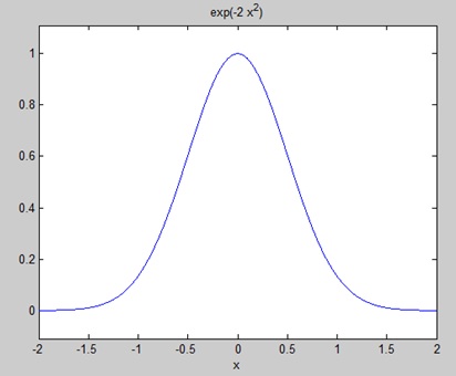
Следующий результат отображается –
FT = (2^(1/2)*pi^(1/2)*exp(-w^2/8))/2
Построение преобразования Фурье как –
ezplot(FT)
Дает следующий график –

Обратные преобразования Фурье
MATLAB предоставляет команду ifourier для вычисления обратного преобразования Фурье функции. Например,
f = ifourier(-2*exp(-abs(w)))
MATLAB выполнит приведенную выше инструкцию и отобразит результат –
f = -2/(pi*(x^2 + 1))
MATLAB – GNU Octave Tutorial
GNU Octave – это язык программирования высокого уровня, такой как MATLAB, и он в основном совместим с MATLAB. Он также используется для численных расчетов.
Octave имеет следующие общие черты с MATLAB:
- матрицы являются фундаментальным типом данных
- имеет встроенную поддержку комплексных чисел
- имеет встроенные математические функции и библиотеки
- поддерживает пользовательские функции
GNU Octave также является свободно распространяемым программным обеспечением. Вы можете распространять его и / или изменять его в соответствии с условиями Стандартной общественной лицензии GNU (GPL), опубликованной Free Software Foundation.
Матлаб против Октавы
Большинство программ MATLAB работают в Octave, но некоторые из программ Octave могут не работать в MATLAB, потому что Octave допускает некоторый синтаксис, которого нет в MATLAB.
Например, MATLAB поддерживает только одинарные кавычки, но Octave поддерживает одинарные и двойные кавычки для определения строк. Если вы ищете учебник по Octave, просим пройти этот учебник с самого начала, который охватывает как MATLAB, так и Octave.
Совместимые примеры
Почти все примеры, описанные в этом руководстве, совместимы как с MATLAB, так и с Octave. Давайте попробуем следующий пример в MATLAB и Octave, который дает тот же результат без каких-либо изменений синтаксиса –
В этом примере создается трехмерная карта поверхности для функции g = xe – (x 2 + y 2 ) . Создайте файл сценария и введите следующий код –
[x,y] = meshgrid(-2:.2:2); g = x .* exp(-x.^2 - y.^2); surf(x, y, g) print -deps graph.eps
Когда вы запускаете файл, MATLAB отображает следующую трехмерную карту –

Несовместимые примеры
Хотя все основные функции MATLAB доступны в Octave, есть некоторые функции, например, Дифференциальное и интеграционное исчисление, которые не совпадают точно в обоих языках. В этом руководстве были приведены примеры обоих типов, в которых они различались по синтаксису.
Рассмотрим следующий пример, где MATLAB и Octave используют разные функции для получения области кривой: f (x) = x 2 cos (x) для −4 ≤ x ≤ 9. Ниже приводится версия кода MATLAB –
f = x^2*cos(x); ezplot(f, [-4,9]) a = int(f, -4, 9) disp('Area: '), disp(double(a));
Когда вы запускаете файл, MATLAB строит график –
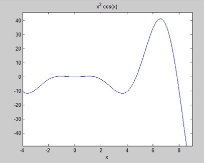
Следующий результат отображается
a = 8*cos(4) + 18*cos(9) + 14*sin(4) + 79*sin(9) Area: 0.3326
Но чтобы дать область той же кривой в Octave, вам придется использовать символический пакет следующим образом:
pkg load symbolic symbols x = sym("x"); f = inline("x^2*cos(x)"); ezplot(f, [-4,9]) print -deps graph.eps [a, ierror, nfneval] = quad(f, -4, 9); display('Area: '), disp(double(a));
МАТЛАБ – Симулинк
Simulink – это среда моделирования и проектирования на основе моделей для динамических и встроенных систем, интегрированная с MATLAB. Simulink, также разработанный MathWorks, представляет собой инструмент языка графического программирования потоков данных для моделирования, моделирования и анализа многодоменных динамических систем. В основном это графический инструмент для построения блок-схем с настраиваемым набором библиотек блоков.
Это позволяет включать алгоритмы MATLAB в модели, а также экспортировать результаты моделирования в MATLAB для дальнейшего анализа.
Simulink поддерживает –
- системный дизайн
- моделирование
- автоматическая генерация кода
- тестирование и проверка встроенных систем
Существует несколько других дополнительных продуктов, предоставляемых MathWorks и сторонними аппаратными и программными продуктами, которые доступны для использования с Simulink.
Следующий список дает краткое описание некоторых из них –
-
Stateflow позволяет разрабатывать конечные автоматы и блок-схемы.
-
Simulink Coder позволяет генерировать исходный код на C для автоматической реализации систем в реальном времени.
-
xPC Target вместе с системами реального времени на базе x86 обеспечивают среду для имитации и тестирования моделей Simulink и Stateflow в реальном времени на физической системе.
-
Встроенный кодер поддерживает определенные встроенные цели.
-
HDL Coder позволяет автоматически генерировать синтезируемые VHDL и Verilog.
-
SimEvents предоставляет библиотеку графических строительных блоков для моделирования систем массового обслуживания.
Stateflow позволяет разрабатывать конечные автоматы и блок-схемы.
Simulink Coder позволяет генерировать исходный код на C для автоматической реализации систем в реальном времени.
xPC Target вместе с системами реального времени на базе x86 обеспечивают среду для имитации и тестирования моделей Simulink и Stateflow в реальном времени на физической системе.
Встроенный кодер поддерживает определенные встроенные цели.
HDL Coder позволяет автоматически генерировать синтезируемые VHDL и Verilog.
SimEvents предоставляет библиотеку графических строительных блоков для моделирования систем массового обслуживания.
Simulink способен систематически проверять и проверять модели посредством проверки стиля моделирования, отслеживания требований и анализа охвата модели.
Simulink Design Verifier позволяет выявлять ошибки проектирования и генерировать сценарии тестирования для проверки модели.
Использование Simulink
Чтобы открыть Simulink, введите рабочее пространство MATLAB –
simulink
Simulink открывается с помощью браузера библиотеки . Браузер библиотеки используется для построения имитационных моделей.

В левой части окна вы найдете несколько библиотек, распределенных по категориям на основе различных систем, щелкнув по каждой из них, вы увидите блоки дизайна на правой панели окна.
Модели зданий
Чтобы создать новую модель, нажмите кнопку « Создать» на панели инструментов браузера библиотеки. Это открывает новое безымянное окно модели.

Модель Simulink – это блок-схема.
Элементы модели добавляются путем выбора соответствующих элементов в браузере библиотеки и перетаскивания их в окно модели.
Кроме того, вы можете скопировать элементы модели и вставить их в окно модели.
Примеры
Перетащите элементы из библиотеки Simulink, чтобы создать свой проект.
В этом примере для моделирования будут использоваться два блока – Источник (сигнал) и Раковина (область). Генератор сигналов (источник) генерирует аналоговый сигнал, который затем будет графически визуализирован областью действия (приемником).
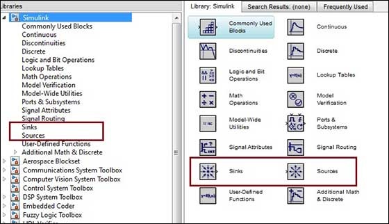
Начните с перетаскивания необходимых блоков из библиотеки в окно проекта. Затем соедините блоки вместе, что можно сделать, перетаскивая соединители из точек соединения одного блока в точки другого.
Давайте перетащим блок «Синусоида» в модель.

Выберите «Sinks» из библиотеки и перетащите блок «Scope» в модель.
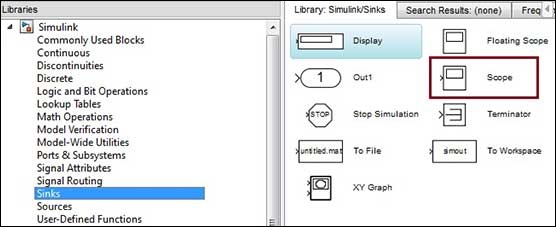
Перетащите сигнальную линию с выхода блока синусоидальной волны на вход блока Scope.

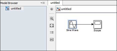
Запустите симуляцию, нажав кнопку « Выполнить », сохраняя все параметры по умолчанию (вы можете изменить их из меню симуляции)
Вы должны получить ниже график из области видимости.
MATLAB — Overview
MATLAB (matrix laboratory) is a fourth-generation high-level programming language and interactive environment for numerical computation, visualization and programming.
MATLAB is developed by MathWorks.
It allows matrix manipulations; plotting of functions and data; implementation of algorithms; creation of user interfaces; interfacing with programs written in other languages, including C, C++, Java, and FORTRAN; analyze data; develop algorithms; and create models and applications.
It has numerous built-in commands and math functions that help you in mathematical calculations, generating plots, and performing numerical methods.
MATLAB’s Power of Computational Mathematics
MATLAB is used in every facet of computational mathematics. Following are some commonly used mathematical calculations where it is used most commonly −
- Dealing with Matrices and Arrays
- 2-D and 3-D Plotting and graphics
- Linear Algebra
- Algebraic Equations
- Non-linear Functions
- Statistics
- Data Analysis
- Calculus and Differential Equations
- Numerical Calculations
- Integration
- Transforms
- Curve Fitting
- Various other special functions
Features of MATLAB
Following are the basic features of MATLAB −
-
It is a high-level language for numerical computation, visualization and application development.
-
It also provides an interactive environment for iterative exploration, design and problem solving.
-
It provides vast library of mathematical functions for linear algebra, statistics, Fourier analysis, filtering, optimization, numerical integration and solving ordinary differential equations.
-
It provides built-in graphics for visualizing data and tools for creating custom plots.
-
MATLAB’s programming interface gives development tools for improving code quality maintainability and maximizing performance.
-
It provides tools for building applications with custom graphical interfaces.
-
It provides functions for integrating MATLAB based algorithms with external applications and languages such as C, Java, .NET and Microsoft Excel.
Uses of MATLAB
MATLAB is widely used as a computational tool in science and engineering encompassing the fields of physics, chemistry, math and all engineering streams. It is used in a range of applications including −
- Signal Processing and Communications
- Image and Video Processing
- Control Systems
- Test and Measurement
- Computational Finance
- Computational Biology
MATLAB — Environment Setup
Local Environment Setup
Setting up MATLAB environment is a matter of few clicks. The installer can be downloaded from here.
MathWorks provides the licensed product, a trial version and a student version as well. You need to log into the site and wait a little for their approval.
After downloading the installer the software can be installed through few clicks.
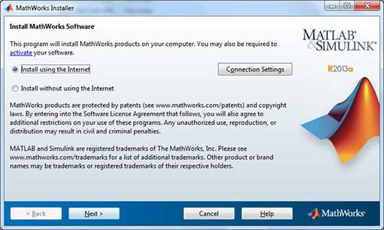

Understanding the MATLAB Environment
MATLAB development IDE can be launched from the icon created on the desktop. The main working window in MATLAB is called the desktop. When MATLAB is started, the desktop appears in its default layout −
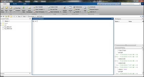
The desktop has the following panels −
-
Current Folder − This panel allows you to access the project folders and files.
-
Command Window − This is the main area where commands can be entered at the command line. It is indicated by the command prompt (>>).
-
Workspace − The workspace shows all the variables created and/or imported from files.
-
Command History − This panel shows or return commands that are entered at the command line.
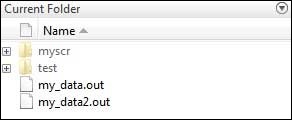
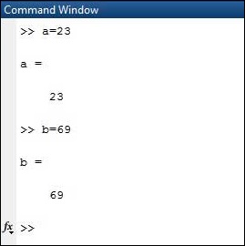

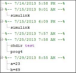
Set up GNU Octave
If you are willing to use Octave on your machine ( Linux, BSD, OS X or Windows ), then kindly download latest version from Download GNU Octave. You can check the given installation instructions for your machine.
MATLAB — Basic Syntax
MATLAB environment behaves like a super-complex calculator. You can enter commands at the >> command prompt.
MATLAB is an interpreted environment. In other words, you give a command and MATLAB executes it right away.
Hands on Practice
Type a valid expression, for example,
5 + 5
And press ENTER
When you click the Execute button, or type Ctrl+E, MATLAB executes it immediately and the result returned is −
ans = 10
Let us take up few more examples −
3 ^ 2 % 3 raised to the power of 2
When you click the Execute button, or type Ctrl+E, MATLAB executes it immediately and the result returned is −
ans = 9
Another example,
sin(pi /2) % sine of angle 90o
When you click the Execute button, or type Ctrl+E, MATLAB executes it immediately and the result returned is −
ans = 1
Another example,
7/0 % Divide by zero
When you click the Execute button, or type Ctrl+E, MATLAB executes it immediately and the result returned is −
ans = Inf warning: division by zero
Another example,
732 * 20.3
When you click the Execute button, or type Ctrl+E, MATLAB executes it immediately and the result returned is −
ans = 1.4860e+04
MATLAB provides some special expressions for some mathematical symbols, like pi for π, Inf for ∞, i (and j) for √-1 etc. Nan stands for ‘not a number’.
Use of Semicolon (;) in MATLAB
Semicolon (;) indicates end of statement. However, if you want to suppress and hide the MATLAB output for an expression, add a semicolon after the expression.
For example,
x = 3; y = x + 5
When you click the Execute button, or type Ctrl+E, MATLAB executes it immediately and the result returned is −
y = 8
Adding Comments
The percent symbol (%) is used for indicating a comment line. For example,
x = 9 % assign the value 9 to x
You can also write a block of comments using the block comment operators % { and % }.
The MATLAB editor includes tools and context menu items to help you add, remove, or change the format of comments.
Commonly used Operators and Special Characters
MATLAB supports the following commonly used operators and special characters −
| Operator | Purpose |
|---|---|
| + | Plus; addition operator. |
| — | Minus; subtraction operator. |
| * | Scalar and matrix multiplication operator. |
| .* | Array multiplication operator. |
| ^ | Scalar and matrix exponentiation operator. |
| .^ | Array exponentiation operator. |
| Left-division operator. | |
| / | Right-division operator. |
| . | Array left-division operator. |
| ./ | Array right-division operator. |
| : | Colon; generates regularly spaced elements and represents an entire row or column. |
| ( ) | Parentheses; encloses function arguments and array indices; overrides precedence. |
| [ ] | Brackets; enclosures array elements. |
| . | Decimal point. |
| … | Ellipsis; line-continuation operator |
| , | Comma; separates statements and elements in a row |
| ; | Semicolon; separates columns and suppresses display. |
| % | Percent sign; designates a comment and specifies formatting. |
| _ | Quote sign and transpose operator. |
| ._ | Nonconjugated transpose operator. |
| = | Assignment operator. |
Special Variables and Constants
MATLAB supports the following special variables and constants −
| Name | Meaning |
|---|---|
| ans | Most recent answer. |
| eps | Accuracy of floating-point precision. |
| i,j | The imaginary unit √-1. |
| Inf | Infinity. |
| NaN | Undefined numerical result (not a number). |
| pi | The number π |
Naming Variables
Variable names consist of a letter followed by any number of letters, digits or underscore.
MATLAB is case-sensitive.
Variable names can be of any length, however, MATLAB uses only first N characters, where N is given by the function namelengthmax.
Saving Your Work
The save command is used for saving all the variables in the workspace, as a file with .mat extension, in the current directory.
For example,
save myfile
You can reload the file anytime later using the load command.
load myfile
MATLAB — Variables
In MATLAB environment, every variable is an array or matrix.
You can assign variables in a simple way. For example,
x = 3 % defining x and initializing it with a value
MATLAB will execute the above statement and return the following result −
x = 3
It creates a 1-by-1 matrix named x and stores the value 3 in its element. Let us check another example,
x = sqrt(16) % defining x and initializing it with an expression
MATLAB will execute the above statement and return the following result −
x = 4
Please note that −
-
Once a variable is entered into the system, you can refer to it later.
-
Variables must have values before they are used.
-
When an expression returns a result that is not assigned to any variable, the system assigns it to a variable named ans, which can be used later.
For example,
sqrt(78)
MATLAB will execute the above statement and return the following result −
ans = 8.8318
You can use this variable ans −
sqrt(78); 9876/ans
MATLAB will execute the above statement and return the following result −
ans = 1118.2
Let’s look at another example −
x = 7 * 8; y = x * 7.89
MATLAB will execute the above statement and return the following result −
y = 441.84
Multiple Assignments
You can have multiple assignments on the same line. For example,
a = 2; b = 7; c = a * b
MATLAB will execute the above statement and return the following result −
c = 14
I have forgotten the Variables!
The who command displays all the variable names you have used.
who
MATLAB will execute the above statement and return the following result −
Your variables are: a ans b c
The whos command displays little more about the variables −
- Variables currently in memory
- Type of each variables
- Memory allocated to each variable
- Whether they are complex variables or not
whos
MATLAB will execute the above statement and return the following result −
Attr Name Size Bytes Class ==== ==== ==== ==== ===== a 1x1 8 double ans 1x70 757 cell b 1x1 8 double c 1x1 8 double Total is 73 elements using 781 bytes
The clear command deletes all (or the specified) variable(s) from the memory.
clear x % it will delete x, won't display anything
clear % it will delete all variables in the workspace
% peacefully and unobtrusively
Long Assignments
Long assignments can be extended to another line by using an ellipses (…). For example,
initial_velocity = 0; acceleration = 9.8; time = 20; final_velocity = initial_velocity + acceleration * time
MATLAB will execute the above statement and return the following result −
final_velocity = 196
The format Command
By default, MATLAB displays numbers with four decimal place values. This is known as short format.
However, if you want more precision, you need to use the format command.
The format long command displays 16 digits after decimal.
For example −
format long x = 7 + 10/3 + 5 ^ 1.2
MATLAB will execute the above statement and return the following result−
x = 17.2319816406394
Another example,
format short x = 7 + 10/3 + 5 ^ 1.2
MATLAB will execute the above statement and return the following result −
x = 17.232
The format bank command rounds numbers to two decimal places. For example,
format bank daily_wage = 177.45; weekly_wage = daily_wage * 6
MATLAB will execute the above statement and return the following result −
weekly_wage = 1064.70
MATLAB displays large numbers using exponential notation.
The format short e command allows displaying in exponential form with four decimal places plus the exponent.
For example,
format short e 4.678 * 4.9
MATLAB will execute the above statement and return the following result −
ans = 2.2922e+01
The format long e command allows displaying in exponential form with four decimal places plus the exponent. For example,
format long e x = pi
MATLAB will execute the above statement and return the following result −
x = 3.141592653589793e+00
The format rat command gives the closest rational expression resulting from a calculation. For example,
format rat 4.678 * 4.9
MATLAB will execute the above statement and return the following result −
ans = 34177/1491
Creating Vectors
A vector is a one-dimensional array of numbers. MATLAB allows creating two types of vectors −
- Row vectors
- Column vectors
Row vectors are created by enclosing the set of elements in square brackets, using space or comma to delimit the elements.
For example,
r = [7 8 9 10 11]
MATLAB will execute the above statement and return the following result −
r = 7 8 9 10 11
Another example,
r = [7 8 9 10 11]; t = [2, 3, 4, 5, 6]; res = r + t
MATLAB will execute the above statement and return the following result −
res =
9 11 13 15 17
Column vectors are created by enclosing the set of elements in square brackets, using semicolon(;) to delimit the elements.
c = [7; 8; 9; 10; 11]
MATLAB will execute the above statement and return the following result −
c =
7
8
9
10
11
Creating Matrices
A matrix is a two-dimensional array of numbers.
In MATLAB, a matrix is created by entering each row as a sequence of space or comma separated elements, and end of a row is demarcated by a semicolon. For example, let us create a 3-by-3 matrix as −
m = [1 2 3; 4 5 6; 7 8 9]
MATLAB will execute the above statement and return the following result −
m =
1 2 3
4 5 6
7 8 9
MATLAB — Commands
MATLAB is an interactive program for numerical computation and data visualization. You can enter a command by typing it at the MATLAB prompt ‘>>’ on the Command Window.
In this section, we will provide lists of commonly used general MATLAB commands.
Commands for Managing a Session
MATLAB provides various commands for managing a session. The following table provides all such commands −
| Command | Purpose |
|---|---|
| clc | Clears command window. |
| clear | Removes variables from memory. |
| exist | Checks for existence of file or variable. |
| global | Declares variables to be global. |
| help | Searches for a help topic. |
| lookfor | Searches help entries for a keyword. |
| quit | Stops MATLAB. |
| who | Lists current variables. |
| whos | Lists current variables (long display). |
Commands for Working with the System
MATLAB provides various useful commands for working with the system, like saving the current work in the workspace as a file and loading the file later.
It also provides various commands for other system-related activities like, displaying date, listing files in the directory, displaying current directory, etc.
The following table displays some commonly used system-related commands −
| Command | Purpose |
|---|---|
| cd | Changes current directory. |
| date | Displays current date. |
| delete | Deletes a file. |
| diary | Switches on/off diary file recording. |
| dir | Lists all files in current directory. |
| load | Loads workspace variables from a file. |
| path | Displays search path. |
| pwd | Displays current directory. |
| save | Saves workspace variables in a file. |
| type | Displays contents of a file. |
| what | Lists all MATLAB files in the current directory. |
| wklread | Reads .wk1 spreadsheet file. |
Input and Output Commands
MATLAB provides the following input and output related commands −
| Command | Purpose |
|---|---|
| disp | Displays contents of an array or string. |
| fscanf | Read formatted data from a file. |
| format | Controls screen-display format. |
| fprintf | Performs formatted writes to screen or file. |
| input | Displays prompts and waits for input. |
| ; | Suppresses screen printing. |
The fscanf and fprintf commands behave like C scanf and printf functions. They support the following format codes −
| Format Code | Purpose |
|---|---|
| %s | Format as a string. |
| %d | Format as an integer. |
| %f | Format as a floating point value. |
| %e | Format as a floating point value in scientific notation. |
| %g | Format in the most compact form: %f or %e. |
| n | Insert a new line in the output string. |
| t | Insert a tab in the output string. |
The format function has the following forms used for numeric display −
| Format Function | Display up to |
|---|---|
| format short | Four decimal digits (default). |
| format long | 16 decimal digits. |
| format short e | Five digits plus exponent. |
| format long e | 16 digits plus exponents. |
| format bank | Two decimal digits. |
| format + | Positive, negative, or zero. |
| format rat | Rational approximation. |
| format compact | Suppresses some line feeds. |
| format loose | Resets to less compact display mode. |
Vector, Matrix and Array Commands
The following table shows various commands used for working with arrays, matrices and vectors −
| Command | Purpose |
|---|---|
| cat | Concatenates arrays. |
| find | Finds indices of nonzero elements. |
| length | Computes number of elements. |
| linspace | Creates regularly spaced vector. |
| logspace | Creates logarithmically spaced vector. |
| max | Returns largest element. |
| min | Returns smallest element. |
| prod | Product of each column. |
| reshape | Changes size. |
| size | Computes array size. |
| sort | Sorts each column. |
| sum | Sums each column. |
| eye | Creates an identity matrix. |
| ones | Creates an array of ones. |
| zeros | Creates an array of zeros. |
| cross | Computes matrix cross products. |
| dot | Computes matrix dot products. |
| det | Computes determinant of an array. |
| inv | Computes inverse of a matrix. |
| pinv | Computes pseudoinverse of a matrix. |
| rank | Computes rank of a matrix. |
| rref | Computes reduced row echelon form. |
| cell | Creates cell array. |
| celldisp | Displays cell array. |
| cellplot | Displays graphical representation of cell array. |
| num2cell | Converts numeric array to cell array. |
| deal | Matches input and output lists. |
| iscell | Identifies cell array. |
Plotting Commands
MATLAB provides numerous commands for plotting graphs. The following table shows some of the commonly used commands for plotting −
| Command | Purpose |
|---|---|
| axis | Sets axis limits. |
| fplot | Intelligent plotting of functions. |
| grid | Displays gridlines. |
| plot | Generates xy plot. |
| Prints plot or saves plot to a file. | |
| title | Puts text at top of plot. |
| xlabel | Adds text label to x-axis. |
| ylabel | Adds text label to y-axis. |
| axes | Creates axes objects. |
| close | Closes the current plot. |
| close all | Closes all plots. |
| figure | Opens a new figure window. |
| gtext | Enables label placement by mouse. |
| hold | Freezes current plot. |
| legend | Legend placement by mouse. |
| refresh | Redraws current figure window. |
| set | Specifies properties of objects such as axes. |
| subplot | Creates plots in subwindows. |
| text | Places string in figure. |
| bar | Creates bar chart. |
| loglog | Creates log-log plot. |
| polar | Creates polar plot. |
| semilogx | Creates semilog plot. (logarithmic abscissa). |
| semilogy | Creates semilog plot. (logarithmic ordinate). |
| stairs | Creates stairs plot. |
| stem | Creates stem plot. |
MATLAB — M-Files
So far, we have used MATLAB environment as a calculator. However, MATLAB is also a powerful programming language, as well as an interactive computational environment.
In previous chapters, you have learned how to enter commands from the MATLAB command prompt. MATLAB also allows you to write series of commands into a file and execute the file as complete unit, like writing a function and calling it.
The M Files
MATLAB allows writing two kinds of program files −
-
Scripts − script files are program files with .m extension. In these files, you write series of commands, which you want to execute together. Scripts do not accept inputs and do not return any outputs. They operate on data in the workspace.
-
Functions − functions files are also program files with .m extension. Functions can accept inputs and return outputs. Internal variables are local to the function.
You can use the MATLAB editor or any other text editor to create your .mfiles. In this section, we will discuss the script files. A script file contains multiple sequential lines of MATLAB commands and function calls. You can run a script by typing its name at the command line.
Creating and Running Script File
To create scripts files, you need to use a text editor. You can open the MATLAB editor in two ways −
- Using the command prompt
- Using the IDE
If you are using the command prompt, type edit in the command prompt. This will open the editor. You can directly type edit and then the filename (with .m extension)
edit Or edit <filename>
The above command will create the file in default MATLAB directory. If you want to store all program files in a specific folder, then you will have to provide the entire path.
Let us create a folder named progs. Type the following commands at the command prompt (>>) −
mkdir progs % create directory progs under default directory chdir progs % changing the current directory to progs edit prog1.m % creating an m file named prog1.m
If you are creating the file for first time, MATLAB prompts you to confirm it. Click Yes.

Alternatively, if you are using the IDE, choose NEW -> Script. This also opens the editor and creates a file named Untitled. You can name and save the file after typing the code.
Type the following code in the editor −
NoOfStudents = 6000; TeachingStaff = 150; NonTeachingStaff = 20; Total = NoOfStudents + TeachingStaff ... + NonTeachingStaff; disp(Total);
After creating and saving the file, you can run it in two ways −
-
Clicking the Run button on the editor window or
-
Just typing the filename (without extension) in the command prompt: >> prog1
The command window prompt displays the result −
6170
Example
Create a script file, and type the following code −
a = 5; b = 7; c = a + b d = c + sin(b) e = 5 * d f = exp(-d)
When the above code is compiled and executed, it produces the following result −
c = 12 d = 12.657 e = 63.285 f = 3.1852e-06
MATLAB — Data Types
MATLAB does not require any type declaration or dimension statements. Whenever MATLAB encounters a new variable name, it creates the variable and allocates appropriate memory space.
If the variable already exists, then MATLAB replaces the original content with new content and allocates new storage space, where necessary.
For example,
Total = 42
The above statement creates a 1-by-1 matrix named ‘Total’ and stores the value 42 in it.
Data Types Available in MATLAB
MATLAB provides 15 fundamental data types. Every data type stores data that is in the form of a matrix or array. The size of this matrix or array is a minimum of 0-by-0 and this can grow up to a matrix or array of any size.
The following table shows the most commonly used data types in MATLAB −
| Sr.No. | Data Type & Description |
|---|---|
| 1 |
int8 8-bit signed integer |
| 2 |
uint8 8-bit unsigned integer |
| 3 |
int16 16-bit signed integer |
| 4 |
uint16 16-bit unsigned integer |
| 5 |
int32 32-bit signed integer |
| 6 |
uint32 32-bit unsigned integer |
| 7 |
int64 64-bit signed integer |
| 8 |
uint64 64-bit unsigned integer |
| 9 |
single single precision numerical data |
| 10 |
double double precision numerical data |
| 11 |
logical logical values of 1 or 0, represent true and false respectively |
| 12 |
char character data (strings are stored as vector of characters) |
| 13 |
cell array array of indexed cells, each capable of storing an array of a different dimension and data type |
| 14 |
structure C-like structures, each structure having named fields capable of storing an array of a different dimension and data type |
| 15 |
function handle pointer to a function |
| 16 |
user classes objects constructed from a user-defined class |
| 17 |
java classes objects constructed from a Java class |
Example
Create a script file with the following code −
str = 'Hello World!' n = 2345 d = double(n) un = uint32(789.50) rn = 5678.92347 c = int32(rn)
When the above code is compiled and executed, it produces the following result −
str = Hello World! n = 2345 d = 2345 un = 790 rn = 5678.9 c = 5679
Data Type Conversion
MATLAB provides various functions for converting, a value from one data type to another. The following table shows the data type conversion functions −
| Function | Purpose |
|---|---|
| char | Convert to character array (string) |
| int2str | Convert integer data to string |
| mat2str | Convert matrix to string |
| num2str | Convert number to string |
| str2double | Convert string to double-precision value |
| str2num | Convert string to number |
| native2unicode | Convert numeric bytes to Unicode characters |
| unicode2native | Convert Unicode characters to numeric bytes |
| base2dec | Convert base N number string to decimal number |
| bin2dec | Convert binary number string to decimal number |
| dec2base | Convert decimal to base N number in string |
| dec2bin | Convert decimal to binary number in string |
| dec2hex | Convert decimal to hexadecimal number in string |
| hex2dec | Convert hexadecimal number string to decimal number |
| hex2num | Convert hexadecimal number string to double-precision number |
| num2hex | Convert singles and doubles to IEEE hexadecimal strings |
| cell2mat | Convert cell array to numeric array |
| cell2struct | Convert cell array to structure array |
| cellstr | Create cell array of strings from character array |
| mat2cell | Convert array to cell array with potentially different sized cells |
| num2cell | Convert array to cell array with consistently sized cells |
| struct2cell | Convert structure to cell array |
Determination of Data Types
MATLAB provides various functions for identifying data type of a variable.
Following table provides the functions for determining the data type of a variable −
| Function | Purpose |
|---|---|
| is | Detect state |
| isa | Determine if input is object of specified class |
| iscell | Determine whether input is cell array |
| iscellstr | Determine whether input is cell array of strings |
| ischar | Determine whether item is character array |
| isfield | Determine whether input is structure array field |
| isfloat | Determine if input is floating-point array |
| ishghandle | True for Handle Graphics object handles |
| isinteger | Determine if input is integer array |
| isjava | Determine if input is Java object |
| islogical | Determine if input is logical array |
| isnumeric | Determine if input is numeric array |
| isobject | Determine if input is MATLAB object |
| isreal | Check if input is real array |
| isscalar | Determine whether input is scalar |
| isstr | Determine whether input is character array |
| isstruct | Determine whether input is structure array |
| isvector | Determine whether input is vector |
| class | Determine class of object |
| validateattributes | Check validity of array |
| whos | List variables in workspace, with sizes and types |
Example
Create a script file with the following code −
x = 3 isinteger(x) isfloat(x) isvector(x) isscalar(x) isnumeric(x) x = 23.54 isinteger(x) isfloat(x) isvector(x) isscalar(x) isnumeric(x) x = [1 2 3] isinteger(x) isfloat(x) isvector(x) isscalar(x) x = 'Hello' isinteger(x) isfloat(x) isvector(x) isscalar(x) isnumeric(x)
When you run the file, it produces the following result −
x = 3
ans = 0
ans = 1
ans = 1
ans = 1
ans = 1
x = 23.540
ans = 0
ans = 1
ans = 1
ans = 1
ans = 1
x =
1 2 3
ans = 0
ans = 1
ans = 1
ans = 0
x = Hello
ans = 0
ans = 0
ans = 1
ans = 0
ans = 0
MATLAB — Operators
An operator is a symbol that tells the compiler to perform specific mathematical or logical manipulations. MATLAB is designed to operate primarily on whole matrices and arrays. Therefore, operators in MATLAB work both on scalar and non-scalar data. MATLAB allows the following types of elementary operations −
- Arithmetic Operators
- Relational Operators
- Logical Operators
- Bitwise Operations
- Set Operations
Arithmetic Operators
MATLAB allows two different types of arithmetic operations −
- Matrix arithmetic operations
- Array arithmetic operations
Matrix arithmetic operations are same as defined in linear algebra. Array operations are executed element by element, both on one-dimensional and multidimensional array.
The matrix operators and array operators are differentiated by the period (.) symbol. However, as the addition and subtraction operation is same for matrices and arrays, the operator is same for both cases. The following table gives brief description of the operators −
Show Examples
| Sr.No. | Operator & Description |
|---|---|
| 1 |
+ Addition or unary plus. A+B adds the values stored in variables A and B. A and B must have the same size, unless one is a scalar. A scalar can be added to a matrix of any size. |
| 2 |
— Subtraction or unary minus. A-B subtracts the value of B from A. A and B must have the same size, unless one is a scalar. A scalar can be subtracted from a matrix of any size. |
| 3 |
* Matrix multiplication. C = A*B is the linear algebraic product of the matrices A and B. More precisely,
For non-scalar A and B, the number of columns of A must be equal to the number of rows of B. A scalar can multiply a matrix of any size. |
| 4 |
.* Array multiplication. A.*B is the element-by-element product of the arrays A and B. A and B must have the same size, unless one of them is a scalar. |
| 5 |
/ Slash or matrix right division. B/A is roughly the same as B*inv(A). More precisely, B/A = (A’B’)’. |
| 6 |
./ Array right division. A./B is the matrix with elements A(i,j)/B(i,j). A and B must have the same size, unless one of them is a scalar. |
| 7 |
Backslash or matrix left division. If A is a square matrix, AB is roughly the same as inv(A)*B, except it is computed in a different way. If A is an n-by-n matrix and B is a column vector with n components, or a matrix with several such columns, then X = AB is the solution to the equation AX = B. A warning message is displayed if A is badly scaled or nearly singular. |
| 8 |
. Array left division. A.B is the matrix with elements B(i,j)/A(i,j). A and B must have the same size, unless one of them is a scalar. |
| 9 |
^ Matrix power. X^p is X to the power p, if p is a scalar. If p is an integer, the power is computed by repeated squaring. If the integer is negative, X is inverted first. For other values of p, the calculation involves eigenvalues and eigenvectors, such that if [V,D] = eig(X), then X^p = V*D.^p/V. |
| 10 |
.^ Array power. A.^B is the matrix with elements A(i,j) to the B(i,j) power. A and B must have the same size, unless one of them is a scalar. |
| 11 |
‘ Matrix transpose. A’ is the linear algebraic transpose of A. For complex matrices, this is the complex conjugate transpose. |
| 12 |
.’ Array transpose. A.’ is the array transpose of A. For complex matrices, this does not involve conjugation. |

Relational Operators
Relational operators can also work on both scalar and non-scalar data. Relational operators for arrays perform element-by-element comparisons between two arrays and return a logical array of the same size, with elements set to logical 1 (true) where the relation is true and elements set to logical 0 (false) where it is not.
The following table shows the relational operators available in MATLAB −
Show Examples
| Sr.No. | Operator & Description |
|---|---|
| 1 |
< Less than |
| 2 |
<= Less than or equal to |
| 3 |
> Greater than |
| 4 |
>= Greater than or equal to |
| 5 |
== Equal to |
| 6 |
~= Not equal to |
Logical Operators
MATLAB offers two types of logical operators and functions −
-
Element-wise − These operators operate on corresponding elements of logical arrays.
-
Short-circuit − These operators operate on scalar and, logical expressions.
Element-wise logical operators operate element-by-element on logical arrays. The symbols &, |, and ~ are the logical array operators AND, OR, and NOT.
Short-circuit logical operators allow short-circuiting on logical operations. The symbols && and || are the logical short-circuit operators AND and OR.
Show Examples
Bitwise Operations
Bitwise operators work on bits and perform bit-by-bit operation. The truth tables for &, |, and ^ are as follows −
| p | q | p & q | p | q | p ^ q |
|---|---|---|---|---|
| 0 | 0 | 0 | 0 | 0 |
| 0 | 1 | 0 | 1 | 1 |
| 1 | 1 | 1 | 1 | 0 |
| 1 | 0 | 0 | 1 | 1 |
Assume if A = 60; and B = 13; Now in binary format they will be as follows −
A = 0011 1100
B = 0000 1101
——————
A&B = 0000 1100
A|B = 0011 1101
A^B = 0011 0001
~A = 1100 0011
MATLAB provides various functions for bit-wise operations like ‘bitwise and’, ‘bitwise or’ and ‘bitwise not’ operations, shift operation, etc.
The following table shows the commonly used bitwise operations −
Show Examples
| Function | Purpose |
|---|---|
| bitand(a, b) | Bit-wise AND of integers a and b |
| bitcmp(a) | Bit-wise complement of a |
| bitget(a,pos) | Get bit at specified position pos, in the integer array a |
| bitor(a, b) | Bit-wise OR of integers a and b |
| bitset(a, pos) | Set bit at specific location pos of a |
| bitshift(a, k) | Returns a shifted to the left by k bits, equivalent to multiplying by 2k. Negative values of k correspond to shifting bits right or dividing by 2|k| and rounding to the nearest integer towards negative infinite. Any overflow bits are truncated. |
| bitxor(a, b) | Bit-wise XOR of integers a and b |
| swapbytes | Swap byte ordering |
Set Operations
MATLAB provides various functions for set operations, like union, intersection and testing for set membership, etc.
The following table shows some commonly used set operations −
Show Examples
| Sr.No. | Function & Description |
|---|---|
| 1 |
intersect(A,B) Set intersection of two arrays; returns the values common to both A and B. The values returned are in sorted order. |
| 2 |
intersect(A,B,’rows’) Treats each row of A and each row of B as single entities and returns the rows common to both A and B. The rows of the returned matrix are in sorted order. |
| 3 |
ismember(A,B) Returns an array the same size as A, containing 1 (true) where the elements of A are found in B. Elsewhere, it returns 0 (false). |
| 4 |
ismember(A,B,’rows’) Treats each row of A and each row of B as single entities and returns a vector containing 1 (true) where the rows of matrix A are also rows of B. Elsewhere, it returns 0 (false). |
| 5 |
issorted(A) Returns logical 1 (true) if the elements of A are in sorted order and logical 0 (false) otherwise. Input A can be a vector or an N-by-1 or 1-by-N cell array of strings. A is considered to be sorted if A and the output of sort(A) are equal. |
| 6 |
issorted(A, ‘rows’) Returns logical 1 (true) if the rows of two-dimensional matrix A is in sorted order, and logical 0 (false) otherwise. Matrix A is considered to be sorted if A and the output of sortrows(A) are equal. |
| 7 |
setdiff(A,B) Sets difference of two arrays; returns the values in A that are not in B. The values in the returned array are in sorted order. |
| 8 |
setdiff(A,B,’rows’) Treats each row of A and each row of B as single entities and returns the rows from A that are not in B. The rows of the returned matrix are in sorted order. The ‘rows’ option does not support cell arrays. |
| 9 |
setxor Sets exclusive OR of two arrays |
| 10 |
union Sets union of two arrays |
| 11 |
unique Unique values in array |
MATLAB — Decision Making
Decision making structures require that the programmer should specify one or more conditions to be evaluated or tested by the program, along with a statement or statements to be executed if the condition is determined to be true, and optionally, other statements to be executed if the condition is determined to be false.
Following is the general form of a typical decision making structure found in most of the programming languages −
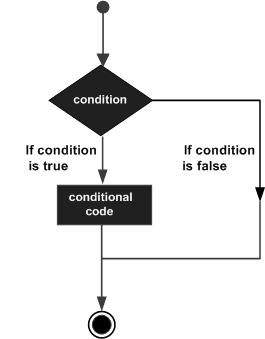
MATLAB provides following types of decision making statements. Click the following links to check their detail −
| Sr.No. | Statement & Description |
|---|---|
| 1 | if … end statement
An if … end statement consists of a boolean expression followed by one or more statements. |
| 2 | if…else…end statement
An if statement can be followed by an optional else statement, which executes when the boolean expression is false. |
| 3 | If… elseif…elseif…else…end statements
An if statement can be followed by one (or more) optional elseif… and an else statement, which is very useful to test various conditions. |
| 4 | nested if statements
You can use one if or elseif statement inside another if or elseif statement(s). |
| 5 | switch statement
A switch statement allows a variable to be tested for equality against a list of values. |
| 6 | nested switch statements
You can use one switch statement inside another switch statement(s). |
MATLAB — Loop Types
There may be a situation when you need to execute a block of code several number of times. In general, statements are executed sequentially. The first statement in a function is executed first, followed by the second, and so on.
Programming languages provide various control structures that allow for more complicated execution paths.
A loop statement allows us to execute a statement or group of statements multiple times and following is the general form of a loop statement in most of the programming languages −

MATLAB provides following types of loops to handle looping requirements. Click the following links to check their detail −
| Sr.No. | Loop Type & Description |
|---|---|
| 1 | while loop
Repeats a statement or group of statements while a given condition is true. It tests the condition before executing the loop body. |
| 2 | for loop
Executes a sequence of statements multiple times and abbreviates the code that manages the loop variable. |
| 3 | nested loops
You can use one or more loops inside any another loop. |
Loop Control Statements
Loop control statements change execution from its normal sequence. When execution leaves a scope, all automatic objects that were created in that scope are destroyed.
MATLAB supports the following control statements. Click the following links to check their detail.
| Sr.No. | Control Statement & Description |
|---|---|
| 1 | break statement
Terminates the loop statement and transfers execution to the statement immediately following the loop. |
| 2 | continue statement
Causes the loop to skip the remainder of its body and immediately retest its condition prior to reiterating. |
MATLAB — Vectors
A vector is a one-dimensional array of numbers. MATLAB allows creating two types of vectors −
- Row vectors
- Column vectors
Row Vectors
Row vectors are created by enclosing the set of elements in square brackets, using space or comma to delimit the elements.
r = [7 8 9 10 11]
MATLAB will execute the above statement and return the following result −
r = 7 8 9 10 11
Column Vectors
Column vectors are created by enclosing the set of elements in square brackets, using semicolon to delimit the elements.
c = [7; 8; 9; 10; 11]
MATLAB will execute the above statement and return the following result −
c =
7
8
9
10
11
Referencing the Elements of a Vector
You can reference one or more of the elements of a vector in several ways. The ith component of a vector v is referred as v(i). For example −
v = [ 1; 2; 3; 4; 5; 6]; % creating a column vector of 6 elements v(3)
MATLAB will execute the above statement and return the following result −
ans = 3
When you reference a vector with a colon, such as v(:), all the components of the vector are listed.
v = [ 1; 2; 3; 4; 5; 6]; % creating a column vector of 6 elements v(:)
MATLAB will execute the above statement and return the following result −
ans =
1
2
3
4
5
6
MATLAB allows you to select a range of elements from a vector.
For example, let us create a row vector rv of 9 elements, then we will reference the elements 3 to 7 by writing rv(3:7) and create a new vector named sub_rv.
rv = [1 2 3 4 5 6 7 8 9]; sub_rv = rv(3:7)
MATLAB will execute the above statement and return the following result −
sub_rv = 3 4 5 6 7
Vector Operations
In this section, let us discuss the following vector operations −
-
Addition and Subtraction of Vectors
-
Scalar Multiplication of Vectors
-
Transpose of a Vector
-
Appending Vectors
-
Magnitude of a Vector
-
Vector Dot Product
-
Vectors with Uniformly Spaced Elements
MATLAB — Matrix
A matrix is a two-dimensional array of numbers.
In MATLAB, you create a matrix by entering elements in each row as comma or space delimited numbers and using semicolons to mark the end of each row.
For example, let us create a 4-by-5 matrix a −
a = [ 1 2 3 4 5; 2 3 4 5 6; 3 4 5 6 7; 4 5 6 7 8]
MATLAB will execute the above statement and return the following result −
a =
1 2 3 4 5
2 3 4 5 6
3 4 5 6 7
4 5 6 7 8
Referencing the Elements of a Matrix
To reference an element in the mth row and nth column, of a matrix mx, we write −
mx(m, n);
For example, to refer to the element in the 2nd row and 5th column, of the matrix a, as created in the last section, we type −
a = [ 1 2 3 4 5; 2 3 4 5 6; 3 4 5 6 7; 4 5 6 7 8]; a(2,5)
MATLAB will execute the above statement and return the following result −
ans = 6
To reference all the elements in the mth column we type A(:,m).
Let us create a column vector v, from the elements of the 4th row of the matrix a −
a = [ 1 2 3 4 5; 2 3 4 5 6; 3 4 5 6 7; 4 5 6 7 8]; v = a(:,4)
MATLAB will execute the above statement and return the following result −
v =
4
5
6
7
You can also select the elements in the mth through nth columns, for this we write −
a(:,m:n)
Let us create a smaller matrix taking the elements from the second and third columns −
a = [ 1 2 3 4 5; 2 3 4 5 6; 3 4 5 6 7; 4 5 6 7 8]; a(:, 2:3)
MATLAB will execute the above statement and return the following result −
ans =
2 3
3 4
4 5
5 6
In the same way, you can create a sub-matrix taking a sub-part of a matrix.
a = [ 1 2 3 4 5; 2 3 4 5 6; 3 4 5 6 7; 4 5 6 7 8]; a(:, 2:3)
MATLAB will execute the above statement and return the following result −
ans =
2 3
3 4
4 5
5 6
In the same way, you can create a sub-matrix taking a sub-part of a matrix.
For example, let us create a sub-matrix sa taking the inner subpart of a −
3 4 5 4 5 6
To do this, write −
a = [ 1 2 3 4 5; 2 3 4 5 6; 3 4 5 6 7; 4 5 6 7 8]; sa = a(2:3,2:4)
MATLAB will execute the above statement and return the following result −
sa =
3 4 5
4 5 6
Deleting a Row or a Column in a Matrix
You can delete an entire row or column of a matrix by assigning an empty set of square braces [] to that row or column. Basically, [] denotes an empty array.
For example, let us delete the fourth row of a −
a = [ 1 2 3 4 5; 2 3 4 5 6; 3 4 5 6 7; 4 5 6 7 8]; a( 4 , : ) = []
MATLAB will execute the above statement and return the following result −
a =
1 2 3 4 5
2 3 4 5 6
3 4 5 6 7
Next, let us delete the fifth column of a −
a = [ 1 2 3 4 5; 2 3 4 5 6; 3 4 5 6 7; 4 5 6 7 8]; a(: , 5)=[]
MATLAB will execute the above statement and return the following result −
a =
1 2 3 4
2 3 4 5
3 4 5 6
4 5 6 7
Example
In this example, let us create a 3-by-3 matrix m, then we will copy the second and third rows of this matrix twice to create a 4-by-3 matrix.
Create a script file with the following code −
a = [ 1 2 3 ; 4 5 6; 7 8 9]; new_mat = a([2,3,2,3],:)
When you run the file, it displays the following result −
new_mat =
4 5 6
7 8 9
4 5 6
7 8 9
Matrix Operations
In this section, let us discuss the following basic and commonly used matrix operations −
-
Addition and Subtraction of Matrices
-
Division of Matrices
-
Scalar Operations of Matrices
-
Transpose of a Matrix
-
Concatenating Matrices
-
Matrix Multiplication
-
Determinant of a Matrix
-
Inverse of a Matrix
MATLAB — Arrays
All variables of all data types in MATLAB are multidimensional arrays. A vector is a one-dimensional array and a matrix is a two-dimensional array.
We have already discussed vectors and matrices. In this chapter, we will discuss multidimensional arrays. However, before that, let us discuss some special types of arrays.
Special Arrays in MATLAB
In this section, we will discuss some functions that create some special arrays. For all these functions, a single argument creates a square array, double arguments create rectangular array.
The zeros() function creates an array of all zeros −
For example −
zeros(5)
MATLAB will execute the above statement and return the following result −
ans =
0 0 0 0 0
0 0 0 0 0
0 0 0 0 0
0 0 0 0 0
0 0 0 0 0
The ones() function creates an array of all ones −
For example −
ones(4,3)
MATLAB will execute the above statement and return the following result −
ans =
1 1 1
1 1 1
1 1 1
1 1 1
The eye() function creates an identity matrix.
For example −
eye(4)
MATLAB will execute the above statement and return the following result −
ans =
1 0 0 0
0 1 0 0
0 0 1 0
0 0 0 1
The rand() function creates an array of uniformly distributed random numbers on (0,1) −
For example −
rand(3, 5)
MATLAB will execute the above statement and return the following result −
ans = 0.8147 0.9134 0.2785 0.9649 0.9572 0.9058 0.6324 0.5469 0.1576 0.4854 0.1270 0.0975 0.9575 0.9706 0.8003
A Magic Square
A magic square is a square that produces the same sum, when its elements are added row-wise, column-wise or diagonally.
The magic() function creates a magic square array. It takes a singular argument that gives the size of the square. The argument must be a scalar greater than or equal to 3.
magic(4)
MATLAB will execute the above statement and return the following result −
ans = 16 2 3 13 5 11 10 8 9 7 6 12 4 14 15 1
Multidimensional Arrays
An array having more than two dimensions is called a multidimensional array in MATLAB. Multidimensional arrays in MATLAB are an extension of the normal two-dimensional matrix.
Generally to generate a multidimensional array, we first create a two-dimensional array and extend it.
For example, let’s create a two-dimensional array a.
a = [7 9 5; 6 1 9; 4 3 2]
MATLAB will execute the above statement and return the following result −
a = 7 9 5 6 1 9 4 3 2
The array a is a 3-by-3 array; we can add a third dimension to a, by providing the values like −
a(:, :, 2)= [ 1 2 3; 4 5 6; 7 8 9]
MATLAB will execute the above statement and return the following result −
a = ans(:,:,1) = 0 0 0 0 0 0 0 0 0 ans(:,:,2) = 1 2 3 4 5 6 7 8 9
We can also create multidimensional arrays using the ones(), zeros() or the rand() functions.
For example,
b = rand(4,3,2)
MATLAB will execute the above statement and return the following result −
b(:,:,1) = 0.0344 0.7952 0.6463 0.4387 0.1869 0.7094 0.3816 0.4898 0.7547 0.7655 0.4456 0.2760 b(:,:,2) = 0.6797 0.4984 0.2238 0.6551 0.9597 0.7513 0.1626 0.3404 0.2551 0.1190 0.5853 0.5060
We can also use the cat() function to build multidimensional arrays. It concatenates a list of arrays along a specified dimension −
Syntax for the cat() function is −
B = cat(dim, A1, A2...)
Where,
-
B is the new array created
-
A1, A2, … are the arrays to be concatenated
-
dim is the dimension along which to concatenate the arrays
Example
Create a script file and type the following code into it −
a = [9 8 7; 6 5 4; 3 2 1]; b = [1 2 3; 4 5 6; 7 8 9]; c = cat(3, a, b, [ 2 3 1; 4 7 8; 3 9 0])
When you run the file, it displays −
c(:,:,1) =
9 8 7
6 5 4
3 2 1
c(:,:,2) =
1 2 3
4 5 6
7 8 9
c(:,:,3) =
2 3 1
4 7 8
3 9 0
Array Functions
MATLAB provides the following functions to sort, rotate, permute, reshape, or shift array contents.
| Function | Purpose |
|---|---|
| length | Length of vector or largest array dimension |
| ndims | Number of array dimensions |
| numel | Number of array elements |
| size | Array dimensions |
| iscolumn | Determines whether input is column vector |
| isempty | Determines whether array is empty |
| ismatrix | Determines whether input is matrix |
| isrow | Determines whether input is row vector |
| isscalar | Determines whether input is scalar |
| isvector | Determines whether input is vector |
| blkdiag | Constructs block diagonal matrix from input arguments |
| circshift | Shifts array circularly |
| ctranspose | Complex conjugate transpose |
| diag | Diagonal matrices and diagonals of matrix |
| flipdim | Flips array along specified dimension |
| fliplr | Flips matrix from left to right |
| flipud | Flips matrix up to down |
| ipermute | Inverses permute dimensions of N-D array |
| permute | Rearranges dimensions of N-D array |
| repmat | Replicates and tile array |
| reshape | Reshapes array |
| rot90 | Rotates matrix 90 degrees |
| shiftdim | Shifts dimensions |
| issorted | Determines whether set elements are in sorted order |
| sort | Sorts array elements in ascending or descending order |
| sortrows | Sorts rows in ascending order |
| squeeze | Removes singleton dimensions |
| transpose | Transpose |
| vectorize | Vectorizes expression |
Examples
The following examples illustrate some of the functions mentioned above.
Length, Dimension and Number of elements −
Create a script file and type the following code into it −
x = [7.1, 3.4, 7.2, 28/4, 3.6, 17, 9.4, 8.9]; length(x) % length of x vector y = rand(3, 4, 5, 2); ndims(y) % no of dimensions in array y s = ['Zara', 'Nuha', 'Shamim', 'Riz', 'Shadab']; numel(s) % no of elements in s
When you run the file, it displays the following result −
ans = 8 ans = 4 ans = 23
Circular Shifting of the Array Elements −
Create a script file and type the following code into it −
a = [1 2 3; 4 5 6; 7 8 9] % the original array a
b = circshift(a,1) % circular shift first dimension values down by 1.
c = circshift(a,[1 -1]) % circular shift first dimension values % down by 1
% and second dimension values to the left % by 1.
When you run the file, it displays the following result −
a = 1 2 3 4 5 6 7 8 9 b = 7 8 9 1 2 3 4 5 6 c = 8 9 7 2 3 1 5 6 4
Sorting Arrays
Create a script file and type the following code into it −
v = [ 23 45 12 9 5 0 19 17] % horizontal vector sort(v) % sorting v m = [2 6 4; 5 3 9; 2 0 1] % two dimensional array sort(m, 1) % sorting m along the row sort(m, 2) % sorting m along the column
When you run the file, it displays the following result −
v = 23 45 12 9 5 0 19 17 ans = 0 5 9 12 17 19 23 45 m = 2 6 4 5 3 9 2 0 1 ans = 2 0 1 2 3 4 5 6 9 ans = 2 4 6 3 5 9 0 1 2
Cell Array
Cell arrays are arrays of indexed cells where each cell can store an array of a different dimensions and data types.
The cell function is used for creating a cell array. Syntax for the cell function is −
C = cell(dim) C = cell(dim1,...,dimN) D = cell(obj)
Where,
-
C is the cell array;
-
dim is a scalar integer or vector of integers that specifies the dimensions of cell array C;
-
dim1, … , dimN are scalar integers that specify the dimensions of C;
-
obj is One of the following −
- Java array or object
- .NET array of type System.String or System.Object
Example
Create a script file and type the following code into it −
c = cell(2, 5);
c = {'Red', 'Blue', 'Green', 'Yellow', 'White'; 1 2 3 4 5}
When you run the file, it displays the following result −
c =
{
[1,1] = Red
[2,1] = 1
[1,2] = Blue
[2,2] = 2
[1,3] = Green
[2,3] = 3
[1,4] = Yellow
[2,4] = 4
[1,5] = White
[2,5] = 5
}
Accessing Data in Cell Arrays
There are two ways to refer to the elements of a cell array −
- Enclosing the indices in first bracket (), to refer to sets of cells
- Enclosing the indices in braces {}, to refer to the data within individual cells
When you enclose the indices in first bracket, it refers to the set of cells.
Cell array indices in smooth parentheses refer to sets of cells.
For example −
c = {'Red', 'Blue', 'Green', 'Yellow', 'White'; 1 2 3 4 5};
c(1:2,1:2)
MATLAB will execute the above statement and return the following result −
ans =
{
[1,1] = Red
[2,1] = 1
[1,2] = Blue
[2,2] = 2
}
You can also access the contents of cells by indexing with curly braces.
For example −
c = {'Red', 'Blue', 'Green', 'Yellow', 'White'; 1 2 3 4 5};
c{1, 2:4}
MATLAB will execute the above statement and return the following result −
ans = Blue ans = Green ans = Yellow
MATLAB — Colon Notation
The colon(:) is one of the most useful operator in MATLAB. It is used to create vectors, subscript arrays, and specify for iterations.
If you want to create a row vector, containing integers from 1 to 10, you write −
1:10
MATLAB executes the statement and returns a row vector containing the integers from 1 to 10 −
ans =
1 2 3 4 5 6 7 8 9 10
If you want to specify an increment value other than one, for example −
100: -5: 50
MATLAB executes the statement and returns the following result −
ans = 100 95 90 85 80 75 70 65 60 55 50
Let us take another example −
0:pi/8:pi
MATLAB executes the statement and returns the following result −
ans =
Columns 1 through 7
0 0.3927 0.7854 1.1781 1.5708 1.9635 2.3562
Columns 8 through 9
2.7489 3.1416
You can use the colon operator to create a vector of indices to select rows, columns or elements of arrays.
The following table describes its use for this purpose (let us have a matrix A) −
| Format | Purpose |
|---|---|
| A(:,j) | is the jth column of A. |
| A(i,:) | is the ith row of A. |
| A(:,:) | is the equivalent two-dimensional array. For matrices this is the same as A. |
| A(j:k) | is A(j), A(j+1),…,A(k). |
| A(:,j:k) | is A(:,j), A(:,j+1),…,A(:,k). |
| A(:,:,k) | is the kth page of three-dimensional array A. |
| A(i,j,k,:) | is a vector in four-dimensional array A. The vector includes A(i,j,k,1), A(i,j,k,2), A(i,j,k,3), and so on. |
| A(:) | is all the elements of A, regarded as a single column. On the left side of an assignment statement, A(:) fills A, preserving its shape from before. In this case, the right side must contain the same number of elements as A. |
Example
Create a script file and type the following code in it −
A = [1 2 3 4; 4 5 6 7; 7 8 9 10] A(:,2) % second column of A A(:,2:3) % second and third column of A A(2:3,2:3) % second and third rows and second and third columns
When you run the file, it displays the following result −
A =
1 2 3 4
4 5 6 7
7 8 9 10
ans =
2
5
8
ans =
2 3
5 6
8 9
ans =
5 6
8 9
MATLAB — Numbers
MATLAB supports various numeric classes that include signed and unsigned integers and single-precision and double-precision floating-point numbers. By default, MATLAB stores all numeric values as double-precision floating point numbers.
You can choose to store any number or array of numbers as integers or as single-precision numbers.
All numeric types support basic array operations and mathematical operations.
Conversion to Various Numeric Data Types
MATLAB provides the following functions to convert to various numeric data types −
| Function | Purpose |
|---|---|
| double | Converts to double precision number |
| single | Converts to single precision number |
| int8 | Converts to 8-bit signed integer |
| int16 | Converts to 16-bit signed integer |
| int32 | Converts to 32-bit signed integer |
| int64 | Converts to 64-bit signed integer |
| uint8 | Converts to 8-bit unsigned integer |
| uint16 | Converts to 16-bit unsigned integer |
| uint32 | Converts to 32-bit unsigned integer |
| uint64 | Converts to 64-bit unsigned integer |
Example
Create a script file and type the following code −
x = single([5.32 3.47 6.28]) .* 7.5 x = double([5.32 3.47 6.28]) .* 7.5 x = int8([5.32 3.47 6.28]) .* 7.5 x = int16([5.32 3.47 6.28]) .* 7.5 x = int32([5.32 3.47 6.28]) .* 7.5 x = int64([5.32 3.47 6.28]) .* 7.5
When you run the file, it shows the following result −
x = 39.900 26.025 47.100 x = 39.900 26.025 47.100 x = 38 23 45 x = 38 23 45 x = 38 23 45 x = 38 23 45
Example
Let us extend the previous example a little more. Create a script file and type the following code −
x = int32([5.32 3.47 6.28]) .* 7.5 x = int64([5.32 3.47 6.28]) .* 7.5 x = num2cell(x)
When you run the file, it shows the following result −
x =
38 23 45
x =
38 23 45
x =
{
[1,1] = 38
[1,2] = 23
[1,3] = 45
}
Smallest and Largest Integers
The functions intmax() and intmin() return the maximum and minimum values that can be represented with all types of integer numbers.
Both the functions take the integer data type as the argument, for example, intmax(int8) or intmin(int64) and return the maximum and minimum values that you can represent with the integer data type.
Example
The following example illustrates how to obtain the smallest and largest values of integers. Create a script file and write the following code in it −
% displaying the smallest and largest signed integer data
str = 'The range for int8 is:nt%d to %d ';
sprintf(str, intmin('int8'), intmax('int8'))
str = 'The range for int16 is:nt%d to %d ';
sprintf(str, intmin('int16'), intmax('int16'))
str = 'The range for int32 is:nt%d to %d ';
sprintf(str, intmin('int32'), intmax('int32'))
str = 'The range for int64 is:nt%d to %d ';
sprintf(str, intmin('int64'), intmax('int64'))
% displaying the smallest and largest unsigned integer data
str = 'The range for uint8 is:nt%d to %d ';
sprintf(str, intmin('uint8'), intmax('uint8'))
str = 'The range for uint16 is:nt%d to %d ';
sprintf(str, intmin('uint16'), intmax('uint16'))
str = 'The range for uint32 is:nt%d to %d ';
sprintf(str, intmin('uint32'), intmax('uint32'))
str = 'The range for uint64 is:nt%d to %d ';
sprintf(str, intmin('uint64'), intmax('uint64'))
When you run the file, it shows the following result −
ans = The range for int8 is: -128 to 127 ans = The range for int16 is: -32768 to 32767 ans = The range for int32 is: -2147483648 to 2147483647 ans = The range for int64 is: 0 to 0 ans = The range for uint8 is: 0 to 255 ans = The range for uint16 is: 0 to 65535 ans = The range for uint32 is: 0 to -1 ans = The range for uint64 is: 0 to 18446744073709551616
Smallest and Largest Floating Point Numbers
The functions realmax() and realmin() return the maximum and minimum values that can be represented with floating point numbers.
Both the functions when called with the argument ‘single’, return the maximum and minimum values that you can represent with the single-precision data type and when called with the argument ‘double’, return the maximum and minimum values that you can represent with the double-precision data type.
Example
The following example illustrates how to obtain the smallest and largest floating point numbers. Create a script file and write the following code in it −
% displaying the smallest and largest single-precision
% floating point number
str = 'The range for single is:nt%g to %g andnt %g to %g';
sprintf(str, -realmax('single'), -realmin('single'), ...
realmin('single'), realmax('single'))
% displaying the smallest and largest double-precision
% floating point number
str = 'The range for double is:nt%g to %g andnt %g to %g';
sprintf(str, -realmax('double'), -realmin('double'), ...
realmin('double'), realmax('double'))
When you run the file, it displays the following result −
ans = The range for single is:
-3.40282e+38 to -1.17549e-38 and
1.17549e-38 to 3.40282e+38
ans = The range for double is:
-1.79769e+308 to -2.22507e-308 and
2.22507e-308 to 1.79769e+308
MATLAB — Strings
Creating a character string is quite simple in MATLAB. In fact, we have used it many times. For example, you type the following in the command prompt −
my_string = 'Tutorials Point'
MATLAB will execute the above statement and return the following result −
my_string = Tutorials Point
MATLAB considers all variables as arrays, and strings are considered as character arrays. Let us use the whos command to check the variable created above −
whos
MATLAB will execute the above statement and return the following result −
Name Size Bytes Class Attributes my_string 1x16 32 char
Interestingly, you can use numeric conversion functions like uint8 or uint16 to convert the characters in the string to their numeric codes. The char function converts the integer vector back to characters −
Example
Create a script file and type the following code into it −
my_string = 'Tutorial''s Point'; str_ascii = uint8(my_string) % 8-bit ascii values str_back_to_char= char(str_ascii) str_16bit = uint16(my_string) % 16-bit ascii values str_back_to_char = char(str_16bit)
When you run the file, it displays the following result −
str_ascii = 84 117 116 111 114 105 97 108 39 115 32 80 111 105 110 116 str_back_to_char = Tutorial's Point str_16bit = 84 117 116 111 114 105 97 108 39 115 32 80 111 105 110 116 str_back_to_char = Tutorial's Point
Rectangular Character Array
The strings we have discussed so far are one-dimensional character arrays; however, we need to store more than that. We need to store more dimensional textual data in our program. This is achieved by creating rectangular character arrays.
Simplest way of creating a rectangular character array is by concatenating two or more one-dimensional character arrays, either vertically or horizontally as required.
You can combine strings vertically in either of the following ways −
-
Using the MATLAB concatenation operator [] and separating each row with a semicolon (;). Please note that in this method each row must contain the same number of characters. For strings with different lengths, you should pad with space characters as needed.
-
Using the char function. If the strings are of different lengths, char pads the shorter strings with trailing blanks so that each row has the same number of characters.
Example
Create a script file and type the following code into it −
doc_profile = ['Zara Ali '; ...
'Sr. Surgeon '; ...
'R N Tagore Cardiology Research Center']
doc_profile = char('Zara Ali', 'Sr. Surgeon', ...
'RN Tagore Cardiology Research Center')
When you run the file, it displays the following result −
doc_profile = Zara Ali Sr. Surgeon R N Tagore Cardiology Research Center doc_profile = Zara Ali Sr. Surgeon RN Tagore Cardiology Research Center
You can combine strings horizontally in either of the following ways −
-
Using the MATLAB concatenation operator, [] and separating the input strings with a comma or a space. This method preserves any trailing spaces in the input arrays.
-
Using the string concatenation function, strcat. This method removes trailing spaces in the inputs.
Example
Create a script file and type the following code into it −
name = 'Zara Ali '; position = 'Sr. Surgeon '; worksAt = 'R N Tagore Cardiology Research Center'; profile = [name ', ' position ', ' worksAt] profile = strcat(name, ', ', position, ', ', worksAt)
When you run the file, it displays the following result −
profile = Zara Ali , Sr. Surgeon , R N Tagore Cardiology Research Center profile = Zara Ali,Sr. Surgeon,R N Tagore Cardiology Research Center
Combining Strings into a Cell Array
From our previous discussion, it is clear that combining strings with different lengths could be a pain as all strings in the array has to be of the same length. We have used blank spaces at the end of strings to equalize their length.
However, a more efficient way to combine the strings is to convert the resulting array into a cell array.
MATLAB cell array can hold different sizes and types of data in an array. Cell arrays provide a more flexible way to store strings of varying length.
The cellstr function converts a character array into a cell array of strings.
Example
Create a script file and type the following code into it −
name = 'Zara Ali '; position = 'Sr. Surgeon '; worksAt = 'R N Tagore Cardiology Research Center'; profile = char(name, position, worksAt); profile = cellstr(profile); disp(profile)
When you run the file, it displays the following result −
{
[1,1] = Zara Ali
[2,1] = Sr. Surgeon
[3,1] = R N Tagore Cardiology Research Center
}
String Functions in MATLAB
MATLAB provides numerous string functions creating, combining, parsing, comparing and manipulating strings.
Following table provides brief description of the string functions in MATLAB −
| Function | Purpose |
|---|---|
| Functions for storing text in character arrays, combine character arrays, etc. | |
| blanks | Create string of blank characters |
| cellstr | Create cell array of strings from character array |
| char | Convert to character array (string) |
| iscellstr | Determine whether input is cell array of strings |
| ischar | Determine whether item is character array |
| sprintf | Format data into string |
| strcat | Concatenate strings horizontally |
| strjoin | Join strings in cell array into single string |
| Functions for identifying parts of strings, find and replace substrings | |
| ischar | Determine whether item is character array |
| isletter | Array elements that are alphabetic letters |
| isspace | Array elements that are space characters |
| isstrprop | Determine whether string is of specified category |
| sscanf | Read formatted data from string |
| strfind | Find one string within another |
| strrep | Find and replace substring |
| strsplit | Split string at specified delimiter |
| strtok | Selected parts of string |
| validatestring | Check validity of text string |
| symvar | Determine symbolic variables in expression |
| regexp | Match regular expression (case sensitive) |
| regexpi | Match regular expression (case insensitive) |
| regexprep | Replace string using regular expression |
| regexptranslate | Translate string into regular expression |
| Functions for string comparison | |
| strcmp | Compare strings (case sensitive) |
| strcmpi | Compare strings (case insensitive) |
| strncmp | Compare first n characters of strings (case sensitive) |
| strncmpi | Compare first n characters of strings (case insensitive) |
| Functions for changing string to upper- or lowercase, creating or removing white space | |
| deblank | Strip trailing blanks from end of string |
| strtrim | Remove leading and trailing white space from string |
| lower | Convert string to lowercase |
| upper | Convert string to uppercase |
| strjust | Justify character array |
Examples
The following examples illustrate some of the above-mentioned string functions −
Formatting Strings
Create a script file and type the following code into it −
A = pi*1000*ones(1,5);
sprintf(' %f n %.2f n %+.2f n %12.2f n %012.2f n', A)
When you run the file, it displays the following result −
ans = 3141.592654
3141.59
+3141.59
3141.59
000003141.59
Joining Strings
Create a script file and type the following code into it −
%cell array of strings
str_array = {'red','blue','green', 'yellow', 'orange'};
% Join strings in cell array into single string
str1 = strjoin(str_array, "-")
str2 = strjoin(str_array, ",")
When you run the file, it displays the following result −
str1 = red-blue-green-yellow-orange str2 = red,blue,green,yellow,orange
Finding and Replacing Strings
Create a script file and type the following code into it −
students = {'Zara Ali', 'Neha Bhatnagar', ...
'Monica Malik', 'Madhu Gautam', ...
'Madhu Sharma', 'Bhawna Sharma',...
'Nuha Ali', 'Reva Dutta', ...
'Sunaina Ali', 'Sofia Kabir'};
% The strrep function searches and replaces sub-string.
new_student = strrep(students(8), 'Reva', 'Poulomi')
% Display first names
first_names = strtok(students)
When you run the file, it displays the following result −
new_student =
{
[1,1] = Poulomi Dutta
}
first_names =
{
[1,1] = Zara
[1,2] = Neha
[1,3] = Monica
[1,4] = Madhu
[1,5] = Madhu
[1,6] = Bhawna
[1,7] = Nuha
[1,8] = Reva
[1,9] = Sunaina
[1,10] = Sofia
}
Comparing Strings
Create a script file and type the following code into it −
str1 = 'This is test'
str2 = 'This is text'
if (strcmp(str1, str2))
sprintf('%s and %s are equal', str1, str2)
else
sprintf('%s and %s are not equal', str1, str2)
end
When you run the file, it displays the following result −
str1 = This is test str2 = This is text ans = This is test and This is text are not equal
MATLAB — Functions
A function is a group of statements that together perform a task. In MATLAB, functions are defined in separate files. The name of the file and of the function should be the same.
Functions operate on variables within their own workspace, which is also called the local workspace, separate from the workspace you access at the MATLAB command prompt which is called the base workspace.
Functions can accept more than one input arguments and may return more than one output arguments.
Syntax of a function statement is −
function [out1,out2, ..., outN] = myfun(in1,in2,in3, ..., inN)
Example
The following function named mymax should be written in a file named mymax.m. It takes five numbers as argument and returns the maximum of the numbers.
Create a function file, named mymax.m and type the following code in it −
function max = mymax(n1, n2, n3, n4, n5) %This function calculates the maximum of the % five numbers given as input max = n1; if(n2 > max) max = n2; end if(n3 > max) max = n3; end if(n4 > max) max = n4; end if(n5 > max) max = n5; end
The first line of a function starts with the keyword function. It gives the name of the function and order of arguments. In our example, the mymax function has five input arguments and one output argument.
The comment lines that come right after the function statement provide the help text. These lines are printed when you type −
help mymax
MATLAB will execute the above statement and return the following result −
This function calculates the maximum of the five numbers given as input
You can call the function as −
mymax(34, 78, 89, 23, 11)
MATLAB will execute the above statement and return the following result −
ans = 89
Anonymous Functions
An anonymous function is like an inline function in traditional programming languages, defined within a single MATLAB statement. It consists of a single MATLAB expression and any number of input and output arguments.
You can define an anonymous function right at the MATLAB command line or within a function or script.
This way you can create simple functions without having to create a file for them.
The syntax for creating an anonymous function from an expression is
f = @(arglist)expression
Example
In this example, we will write an anonymous function named power, which will take two numbers as input and return first number raised to the power of the second number.
Create a script file and type the following code in it −
power = @(x, n) x.^n; result1 = power(7, 3) result2 = power(49, 0.5) result3 = power(10, -10) result4 = power (4.5, 1.5)
When you run the file, it displays −
result1 = 343 result2 = 7 result3 = 1.0000e-10 result4 = 9.5459
Primary and Sub-Functions
Any function other than an anonymous function must be defined within a file. Each function file contains a required primary function that appears first and any number of optional sub-functions that comes after the primary function and used by it.
Primary functions can be called from outside of the file that defines them, either from command line or from other functions, but sub-functions cannot be called from command line or other functions, outside the function file.
Sub-functions are visible only to the primary function and other sub-functions within the function file that defines them.
Example
Let us write a function named quadratic that would calculate the roots of a quadratic equation. The function would take three inputs, the quadratic co-efficient, the linear co-efficient and the constant term. It would return the roots.
The function file quadratic.m will contain the primary function quadratic and the sub-function disc, which calculates the discriminant.
Create a function file quadratic.m and type the following code in it −
function [x1,x2] = quadratic(a,b,c) %this function returns the roots of % a quadratic equation. % It takes 3 input arguments % which are the co-efficients of x2, x and the %constant term % It returns the roots d = disc(a,b,c); x1 = (-b + d) / (2*a); x2 = (-b - d) / (2*a); end % end of quadratic function dis = disc(a,b,c) %function calculates the discriminant dis = sqrt(b^2 - 4*a*c); end % end of sub-function
You can call the above function from command prompt as −
quadratic(2,4,-4)
MATLAB will execute the above statement and return the following result −
ans = 0.7321
Nested Functions
You can define functions within the body of another function. These are called nested functions. A nested function contains any or all of the components of any other function.
Nested functions are defined within the scope of another function and they share access to the containing function’s workspace.
A nested function follows the following syntax −
function x = A(p1, p2) ... B(p2) function y = B(p3) ... end ... end
Example
Let us rewrite the function quadratic, from previous example, however, this time the disc function will be a nested function.
Create a function file quadratic2.m and type the following code in it −
function [x1,x2] = quadratic2(a,b,c) function disc % nested function d = sqrt(b^2 - 4*a*c); end % end of function disc disc; x1 = (-b + d) / (2*a); x2 = (-b - d) / (2*a); end % end of function quadratic2
You can call the above function from command prompt as −
quadratic2(2,4,-4)
MATLAB will execute the above statement and return the following result −
ans = 0.73205
Private Functions
A private function is a primary function that is visible only to a limited group of other functions. If you do not want to expose the implementation of a function(s), you can create them as private functions.
Private functions reside in subfolders with the special name private.
They are visible only to functions in the parent folder.
Example
Let us rewrite the quadratic function. This time, however, the disc function calculating the discriminant, will be a private function.
Create a subfolder named private in working directory. Store the following function file disc.m in it −
function dis = disc(a,b,c) %function calculates the discriminant dis = sqrt(b^2 - 4*a*c); end % end of sub-function
Create a function quadratic3.m in your working directory and type the following code in it −
function [x1,x2] = quadratic3(a,b,c) %this function returns the roots of % a quadratic equation. % It takes 3 input arguments % which are the co-efficient of x2, x and the %constant term % It returns the roots d = disc(a,b,c); x1 = (-b + d) / (2*a); x2 = (-b - d) / (2*a); end % end of quadratic3
You can call the above function from command prompt as −
quadratic3(2,4,-4)
MATLAB will execute the above statement and return the following result −
ans = 0.73205
Global Variables
Global variables can be shared by more than one function. For this, you need to declare the variable as global in all the functions.
If you want to access that variable from the base workspace, then declare the variable at the command line.
The global declaration must occur before the variable is actually used in a function. It is a good practice to use capital letters for the names of global variables to distinguish them from other variables.
Example
Let us create a function file named average.m and type the following code in it −
function avg = average(nums) global TOTAL avg = sum(nums)/TOTAL; end
Create a script file and type the following code in it −
global TOTAL; TOTAL = 10; n = [34, 45, 25, 45, 33, 19, 40, 34, 38, 42]; av = average(n)
When you run the file, it will display the following result −
av = 35.500
MATLAB — Data Import
Importing data in MATLAB means loading data from an external file. The importdata function allows loading various data files of different formats. It has the following five forms −
| Sr.No. | Function & Description |
|---|---|
| 1 |
A = importdata(filename) Loads data into array A from the file denoted by filename. |
| 2 |
A = importdata(‘-pastespecial’) Loads data from the system clipboard rather than from a file. |
| 3 |
A = importdata(___, delimiterIn) Interprets delimiterIn as the column separator in ASCII file, filename, or the clipboard data. You can use delimiterIn with any of the input arguments in the above syntaxes. |
| 4 |
A = importdata(___, delimiterIn, headerlinesIn) Loads data from ASCII file, filename, or the clipboard, reading numeric data starting from line headerlinesIn+1. |
| 5 |
[A, delimiterOut, headerlinesOut] = importdata(___) Returns the detected delimiter character for the input ASCII file in delimiterOut and the detected number of header lines in headerlinesOut, using any of the input arguments in the previous syntaxes. |
By default, Octave does not have support for importdata() function, so you will have to search and install this package to make following examples work with your Octave installation.
Example 1
Let us load and display an image file. Create a script file and type the following code in it −
filename = 'smile.jpg'; A = importdata(filename); image(A);
When you run the file, MATLAB displays the image file. However, you must store it in the current directory.

Example 2
In this example, we import a text file and specify Delimiter and Column Header. Let us create a space-delimited ASCII file with column headers, named weeklydata.txt.
Our text file weeklydata.txt looks like this −
SunDay MonDay TuesDay WednesDay ThursDay FriDay SaturDay 95.01 76.21 61.54 40.57 55.79 70.28 81.53 73.11 45.65 79.19 93.55 75.29 69.87 74.68 60.68 41.85 92.18 91.69 81.32 90.38 74.51 48.60 82.14 73.82 41.03 0.99 67.22 93.18 89.13 44.47 57.63 89.36 13.89 19.88 46.60
Create a script file and type the following code in it −
filename = 'weeklydata.txt';
delimiterIn = ' ';
headerlinesIn = 1;
A = importdata(filename,delimiterIn,headerlinesIn);
% View data
for k = [1:7]
disp(A.colheaders{1, k})
disp(A.data(:, k))
disp(' ')
end
When you run the file, it displays the following result −
SunDay 95.0100 73.1100 60.6800 48.6000 89.1300 MonDay 76.2100 45.6500 41.8500 82.1400 44.4700 TuesDay 61.5400 79.1900 92.1800 73.8200 57.6300 WednesDay 40.5700 93.5500 91.6900 41.0300 89.3600 ThursDay 55.7900 75.2900 81.3200 0.9900 13.8900 FriDay 70.2800 69.8700 90.3800 67.2200 19.8800 SaturDay 81.5300 74.6800 74.5100 93.1800 46.6000
Example 3
In this example, let us import data from clipboard.
Copy the following lines to the clipboard −
Mathematics is simple
Create a script file and type the following code −
A = importdata('-pastespecial')
When you run the file, it displays the following result −
A = 'Mathematics is simple'
Low-Level File I/O
The importdata function is a high-level function. The low-level file I/O functions in MATLAB allow the most control over reading or writing data to a file. However, these functions need more detailed information about your file to work efficiently.
MATLAB provides the following functions for read and write operations at the byte or character level −
| Function | Description |
|---|---|
| fclose | Close one or all open files |
| feof | Test for end-of-file |
| ferror | Information about file I/O errors |
| fgetl | Read line from file, removing newline characters |
| fgets | Read line from file, keeping newline characters |
| fopen | Open file, or obtain information about open files |
| fprintf | Write data to text file |
| fread | Read data from binary file |
| frewind | Move file position indicator to beginning of open file |
| fscanf | Read data from text file |
| fseek | Move to specified position in file |
| ftell | Position in open file |
| fwrite | Write data to binary file |
Import Text Data Files with Low-Level I/O
MATLAB provides the following functions for low-level import of text data files −
-
The fscanf function reads formatted data in a text or ASCII file.
-
The fgetl and fgets functions read one line of a file at a time, where a newline character separates each line.
-
The fread function reads a stream of data at the byte or bit level.
Example
We have a text data file ‘myfile.txt’ saved in our working directory. The file stores rainfall data for three months; June, July and August for the year 2012.
The data in myfile.txt contains repeated sets of time, month and rainfall measurements at five places. The header data stores the number of months M; so we have M sets of measurements.
The file looks like this −
Rainfall Data Months: June, July, August M = 3 12:00:00 June-2012 17.21 28.52 39.78 16.55 23.67 19.15 0.35 17.57 NaN 12.01 17.92 28.49 17.40 17.06 11.09 9.59 9.33 NaN 0.31 0.23 10.46 13.17 NaN 14.89 19.33 20.97 19.50 17.65 14.45 14.00 18.23 10.34 17.95 16.46 19.34 09:10:02 July-2012 12.76 16.94 14.38 11.86 16.89 20.46 23.17 NaN 24.89 19.33 30.97 49.50 47.65 24.45 34.00 18.23 30.34 27.95 16.46 19.34 30.46 33.17 NaN 34.89 29.33 30.97 49.50 47.65 24.45 34.00 28.67 30.34 27.95 36.46 29.34 15:03:40 August-2012 17.09 16.55 19.59 17.25 19.22 17.54 11.45 13.48 22.55 24.01 NaN 21.19 25.85 25.05 27.21 26.79 24.98 12.23 16.99 18.67 17.54 11.45 13.48 22.55 24.01 NaN 21.19 25.85 25.05 27.21 26.79 24.98 12.23 16.99 18.67
We will import data from this file and display this data. Take the following steps −
-
Open the file with fopen function and get the file identifier.
-
Describe the data in the file with format specifiers, such as ‘%s‘ for a string, ‘%d‘ for an integer, or ‘%f‘ for a floating-point number.
-
To skip literal characters in the file, include them in the format description. To skip a data field, use an asterisk (‘*’) in the specifier.
For example, to read the headers and return the single value for M, we write −
M = fscanf(fid, '%*s %*sn%*s %*s %*s %*snM=%dnn', 1);
-
By default, fscanf reads data according to our format description until it does not find any match for the data, or it reaches the end of the file. Here we will use for loop for reading 3 sets of data and each time, it will read 7 rows and 5 columns.
-
We will create a structure named mydata in the workspace to store data read from the file. This structure has three fields — time, month, and raindata array.
Create a script file and type the following code in it −
filename = '/data/myfile.txt';
rows = 7;
cols = 5;
% open the file
fid = fopen(filename);
% read the file headers, find M (number of months)
M = fscanf(fid, '%*s %*sn%*s %*s %*s %*snM=%dnn', 1);
% read each set of measurements
for n = 1:M
mydata(n).time = fscanf(fid, '%s', 1);
mydata(n).month = fscanf(fid, '%s', 1);
% fscanf fills the array in column order,
% so transpose the results
mydata(n).raindata = ...
fscanf(fid, '%f', [rows, cols]);
end
for n = 1:M
disp(mydata(n).time), disp(mydata(n).month)
disp(mydata(n).raindata)
end
% close the file
fclose(fid);
When you run the file, it displays the following result −
12:00:00 June-2012 17.2100 17.5700 11.0900 13.1700 14.4500 28.5200 NaN 9.5900 NaN 14.0000 39.7800 12.0100 9.3300 14.8900 18.2300 16.5500 17.9200 NaN 19.3300 10.3400 23.6700 28.4900 0.3100 20.9700 17.9500 19.1500 17.4000 0.2300 19.5000 16.4600 0.3500 17.0600 10.4600 17.6500 19.3400 09:10:02 July-2012 12.7600 NaN 34.0000 33.1700 24.4500 16.9400 24.8900 18.2300 NaN 34.0000 14.3800 19.3300 30.3400 34.8900 28.6700 11.8600 30.9700 27.9500 29.3300 30.3400 16.8900 49.5000 16.4600 30.9700 27.9500 20.4600 47.6500 19.3400 49.5000 36.4600 23.1700 24.4500 30.4600 47.6500 29.3400 15:03:40 August-2012 17.0900 13.4800 27.2100 11.4500 25.0500 16.5500 22.5500 26.7900 13.4800 27.2100 19.5900 24.0100 24.9800 22.5500 26.7900 17.2500 NaN 12.2300 24.0100 24.9800 19.2200 21.1900 16.9900 NaN 12.2300 17.5400 25.8500 18.6700 21.1900 16.9900 11.4500 25.0500 17.5400 25.8500 18.6700
MATLAB — Data Output
Data export (or output) in MATLAB means to write into files. MATLAB allows you to use your data in another application that reads ASCII files. For this, MATLAB provides several data export options.
You can create the following type of files −
-
Rectangular, delimited ASCII data file from an array.
-
Diary (or log) file of keystrokes and the resulting text output.
-
Specialized ASCII file using low-level functions such as fprintf.
-
MEX-file to access your C/C++ or Fortran routine that writes to a particular text file format.
Apart from this, you can also export data to spreadsheets.
There are two ways to export a numeric array as a delimited ASCII data file −
-
Using the save function and specifying the -ascii qualifier
-
Using the dlmwrite function
Syntax for using the save function is −
save my_data.out num_array -ascii
where, my_data.out is the delimited ASCII data file created, num_array is a numeric array and −ascii is the specifier.
Syntax for using the dlmwrite function is −
dlmwrite('my_data.out', num_array, 'dlm_char')
where, my_data.out is the delimited ASCII data file created, num_array is a numeric array and dlm_char is the delimiter character.
Example
The following example demonstrates the concept. Create a script file and type the following code −
num_array = [ 1 2 3 4 ; 4 5 6 7; 7 8 9 0];
save array_data1.out num_array -ascii;
type array_data1.out
dlmwrite('array_data2.out', num_array, ' ');
type array_data2.out
When you run the file, it displays the following result −
1.0000000e+00 2.0000000e+00 3.0000000e+00 4.0000000e+00 4.0000000e+00 5.0000000e+00 6.0000000e+00 7.0000000e+00 7.0000000e+00 8.0000000e+00 9.0000000e+00 0.0000000e+00 1 2 3 4 4 5 6 7 7 8 9 0
Please note that the save -ascii command and the dlmwrite function does not work with cell arrays as input. To create a delimited ASCII file from the contents of a cell array, you can
-
Either, convert the cell array to a matrix using the cell2mat function
-
Or export the cell array using low-level file I/O functions.
If you use the save function to write a character array to an ASCII file, it writes the ASCII equivalent of the characters to the file.
For example, let us write the word ‘hello’ to a file −
h = 'hello'; save textdata.out h -ascii type textdata.out
MATLAB executes the above statements and displays the following result. which is the characters of the string ‘hello’ in 8-digit ASCII format.
1.0400000e+02 1.0100000e+02 1.0800000e+02 1.0800000e+02 1.1100000e+02
Writing to Diary Files
Diary files are activity logs of your MATLAB session. The diary function creates an exact copy of your session in a disk file, excluding graphics.
To turn on the diary function, type −
diary
Optionally, you can give the name of the log file, say −
diary logdata.out
To turn off the diary function −
diary off
You can open the diary file in a text editor.
Exporting Data to Text Data Files with Low-Level I/O
So far, we have exported numeric arrays. However, you may need to create other text files, including combinations of numeric and character data, nonrectangular output files, or files with non-ASCII encoding schemes. For these purposes, MATLAB provides the low-level fprintf function.
As in low-level I/O file activities, before exporting, you need to open or create a file with the fopen function and get the file identifier. By default, fopen opens a file for read-only access. You should specify the permission to write or append, such as ‘w’ or ‘a’.
After processing the file, you need to close it with fclose(fid) function.
The following example demonstrates the concept −
Example
Create a script file and type the following code in it −
% create a matrix y, with two rows
x = 0:10:100;
y = [x; log(x)];
% open a file for writing
fid = fopen('logtable.txt', 'w');
% Table Header
fprintf(fid, 'Log Functionnn');
% print values in column order
% two values appear on each row of the file
fprintf(fid, '%f %fn', y);
fclose(fid);
% display the file created
type logtable.txt
When you run the file, it displays the following result −
Log Function 0.000000 -Inf 10.000000 2.302585 20.000000 2.995732 30.000000 3.401197 40.000000 3.688879 50.000000 3.912023 60.000000 4.094345 70.000000 4.248495 80.000000 4.382027 90.000000 4.499810 100.000000 4.605170
MATLAB — Plotting
To plot the graph of a function, you need to take the following steps −
-
Define x, by specifying the range of values for the variable x, for which the function is to be plotted
-
Define the function, y = f(x)
-
Call the plot command, as plot(x, y)
Following example would demonstrate the concept. Let us plot the simple function y = x for the range of values for x from 0 to 100, with an increment of 5.
Create a script file and type the following code −
x = [0:5:100]; y = x; plot(x, y)
When you run the file, MATLAB displays the following plot −

Let us take one more example to plot the function y = x2. In this example, we will draw two graphs with the same function, but in second time, we will reduce the value of increment. Please note that as we decrease the increment, the graph becomes smoother.
Create a script file and type the following code −
x = [1 2 3 4 5 6 7 8 9 10]; x = [-100:20:100]; y = x.^2; plot(x, y)
When you run the file, MATLAB displays the following plot −

Change the code file a little, reduce the increment to 5 −
x = [-100:5:100]; y = x.^2; plot(x, y)
MATLAB draws a smoother graph −

Adding Title, Labels, Grid Lines and Scaling on the Graph
MATLAB allows you to add title, labels along the x-axis and y-axis, grid lines and also to adjust the axes to spruce up the graph.
-
The xlabel and ylabel commands generate labels along x-axis and y-axis.
-
The title command allows you to put a title on the graph.
-
The grid on command allows you to put the grid lines on the graph.
-
The axis equal command allows generating the plot with the same scale factors and the spaces on both axes.
-
The axis square command generates a square plot.
Example
Create a script file and type the following code −
x = [0:0.01:10];
y = sin(x);
plot(x, y), xlabel('x'), ylabel('Sin(x)'), title('Sin(x) Graph'),
grid on, axis equal
MATLAB generates the following graph −
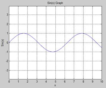
Drawing Multiple Functions on the Same Graph
You can draw multiple graphs on the same plot. The following example demonstrates the concept −
Example
Create a script file and type the following code −
x = [0 : 0.01: 10];
y = sin(x);
g = cos(x);
plot(x, y, x, g, '.-'), legend('Sin(x)', 'Cos(x)')
MATLAB generates the following graph −
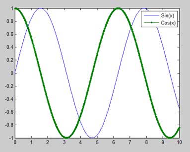
Setting Colors on Graph
MATLAB provides eight basic color options for drawing graphs. The following table shows the colors and their codes −
| Code | Color |
|---|---|
| w | White |
| k | Black |
| b | Blue |
| r | Red |
| c | Cyan |
| g | Green |
| m | Magenta |
| y | Yellow |
Example
Let us draw the graph of two polynomials
-
f(x) = 3x4 + 2x3+ 7x2 + 2x + 9 and
-
g(x) = 5x3 + 9x + 2
Create a script file and type the following code −
x = [-10 : 0.01: 10]; y = 3*x.^4 + 2 * x.^3 + 7 * x.^2 + 2 * x + 9; g = 5 * x.^3 + 9 * x + 2; plot(x, y, 'r', x, g, 'g')
When you run the file, MATLAB generates the following graph −

Setting Axis Scales
The axis command allows you to set the axis scales. You can provide minimum and maximum values for x and y axes using the axis command in the following way −
axis ( [xmin xmax ymin ymax] )
The following example shows this −
Example
Create a script file and type the following code −
x = [0 : 0.01: 10]; y = exp(-x).* sin(2*x + 3); plot(x, y), axis([0 10 -1 1])
When you run the file, MATLAB generates the following graph −

Generating Sub-Plots
When you create an array of plots in the same figure, each of these plots is called a subplot. The subplot command is used for creating subplots.
Syntax for the command is −
subplot(m, n, p)
where, m and n are the number of rows and columns of the plot array and p specifies where to put a particular plot.
Each plot created with the subplot command can have its own characteristics. Following example demonstrates the concept −
Example
Let us generate two plots −
y = e−1.5xsin(10x)
y = e−2xsin(10x)
Create a script file and type the following code −
x = [0:0.01:5];
y = exp(-1.5*x).*sin(10*x);
subplot(1,2,1)
plot(x,y), xlabel('x'),ylabel('exp(–1.5x)*sin(10x)'),axis([0 5 -1 1])
y = exp(-2*x).*sin(10*x);
subplot(1,2,2)
plot(x,y),xlabel('x'),ylabel('exp(–2x)*sin(10x)'),axis([0 5 -1 1])
When you run the file, MATLAB generates the following graph −
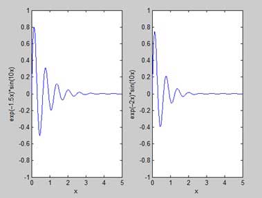
MATLAB — Graphics
This chapter will continue exploring the plotting and graphics capabilities of MATLAB. We will discuss −
- Drawing bar charts
- Drawing contours
- Three dimensional plots
Drawing Bar Charts
The bar command draws a two dimensional bar chart. Let us take up an example to demonstrate the idea.
Example
Let us have an imaginary classroom with 10 students. We know the percent of marks obtained by these students are 75, 58, 90, 87, 50, 85, 92, 75, 60 and 95. We will draw the bar chart for this data.
Create a script file and type the following code −
x = [1:10];
y = [75, 58, 90, 87, 50, 85, 92, 75, 60, 95];
bar(x,y), xlabel('Student'),ylabel('Score'),
title('First Sem:')
print -deps graph.eps
When you run the file, MATLAB displays the following bar chart −

Drawing Contours
A contour line of a function of two variables is a curve along which the function has a constant value. Contour lines are used for creating contour maps by joining points of equal elevation above a given level, such as mean sea level.
MATLAB provides a contour function for drawing contour maps.
Example
Let us generate a contour map that shows the contour lines for a given function g = f(x, y). This function has two variables. So, we will have to generate two independent variables, i.e., two data sets x and y. This is done by calling the meshgrid command.
The meshgrid command is used for generating a matrix of elements that give the range over x and y along with the specification of increment in each case.
Let us plot our function g = f(x, y), where −5 ≤ x ≤ 5, −3 ≤ y ≤ 3. Let us take an increment of 0.1 for both the values. The variables are set as −
[x,y] = meshgrid(–5:0.1:5, –3:0.1:3);
Lastly, we need to assign the function. Let our function be: x2 + y2
Create a script file and type the following code −
[x,y] = meshgrid(-5:0.1:5,-3:0.1:3); %independent variables g = x.^2 + y.^2; % our function contour(x,y,g) % call the contour function print -deps graph.eps
When you run the file, MATLAB displays the following contour map −
Let us modify the code a little to spruce up the map
[x,y] = meshgrid(-5:0.1:5,-3:0.1:3); %independent variables g = x.^2 + y.^2; % our function [C, h] = contour(x,y,g); % call the contour function set(h,'ShowText','on','TextStep',get(h,'LevelStep')*2) print -deps graph.eps
When you run the file, MATLAB displays the following contour map −

Three Dimensional Plots
Three-dimensional plots basically display a surface defined by a function in two variables, g = f (x,y).
As before, to define g, we first create a set of (x,y) points over the domain of the function using the meshgrid command. Next, we assign the function itself. Finally, we use the surf command to create a surface plot.
The following example demonstrates the concept −
Example
Let us create a 3D surface map for the function g = xe-(x2 + y2)
Create a script file and type the following code −
[x,y] = meshgrid(-2:.2:2); g = x .* exp(-x.^2 - y.^2); surf(x, y, g) print -deps graph.eps
When you run the file, MATLAB displays the following 3-D map −

You can also use the mesh command to generate a three-dimensional surface. However, the surf command displays both the connecting lines and the faces of the surface in color, whereas, the mesh command creates a wireframe surface with colored lines connecting the defining points.
MATLAB — Algebra
So far, we have seen that all the examples work in MATLAB as well as its GNU, alternatively called Octave. But for solving basic algebraic equations, both MATLAB and Octave are little different, so we will try to cover MATLAB and Octave in separate sections.
We will also discuss factorizing and simplification of algebraic expressions.
Solving Basic Algebraic Equations in MATLAB
The solve function is used for solving algebraic equations. In its simplest form, the solve function takes the equation enclosed in quotes as an argument.
For example, let us solve for x in the equation x-5 = 0
solve('x-5=0')
MATLAB will execute the above statement and return the following result −
ans = 5
You can also call the solve function as −
y = solve('x-5 = 0')
MATLAB will execute the above statement and return the following result −
y = 5
You may even not include the right hand side of the equation −
solve('x-5')
MATLAB will execute the above statement and return the following result −
ans = 5
If the equation involves multiple symbols, then MATLAB by default assumes that you are solving for x, however, the solve function has another form −
solve(equation, variable)
where, you can also mention the variable.
For example, let us solve the equation v – u – 3t2 = 0, for v. In this case, we should write −
solve('v-u-3*t^2=0', 'v')
MATLAB will execute the above statement and return the following result −
ans = 3*t^2 + u
Solving Basic Algebraic Equations in Octave
The roots function is used for solving algebraic equations in Octave and you can write above examples as follows −
For example, let us solve for x in the equation x-5 = 0
roots([1, -5])
Octave will execute the above statement and return the following result −
ans = 5
You can also call the solve function as −
y = roots([1, -5])
Octave will execute the above statement and return the following result −
y = 5
Solving Quadratic Equations in MATLAB
The solve function can also solve higher order equations. It is often used to solve quadratic equations. The function returns the roots of the equation in an array.
The following example solves the quadratic equation x2 -7x +12 = 0. Create a script file and type the following code −
eq = 'x^2 -7*x + 12 = 0';
s = solve(eq);
disp('The first root is: '), disp(s(1));
disp('The second root is: '), disp(s(2));
When you run the file, it displays the following result −
The first root is: 3 The second root is: 4
Solving Quadratic Equations in Octave
The following example solves the quadratic equation x2 -7x +12 = 0 in Octave. Create a script file and type the following code −
s = roots([1, -7, 12]);
disp('The first root is: '), disp(s(1));
disp('The second root is: '), disp(s(2));
When you run the file, it displays the following result −
The first root is: 4 The second root is: 3
Solving Higher Order Equations in MATLAB
The solve function can also solve higher order equations. For example, let us solve a cubic equation as (x-3)2(x-7) = 0
solve('(x-3)^2*(x-7)=0')
MATLAB will execute the above statement and return the following result −
ans = 3 3 7
In case of higher order equations, roots are long containing many terms. You can get the numerical value of such roots by converting them to double. The following example solves the fourth order equation x4 − 7x3 + 3x2 − 5x + 9 = 0.
Create a script file and type the following code −
eq = 'x^4 - 7*x^3 + 3*x^2 - 5*x + 9 = 0';
s = solve(eq);
disp('The first root is: '), disp(s(1));
disp('The second root is: '), disp(s(2));
disp('The third root is: '), disp(s(3));
disp('The fourth root is: '), disp(s(4));
% converting the roots to double type
disp('Numeric value of first root'), disp(double(s(1)));
disp('Numeric value of second root'), disp(double(s(2)));
disp('Numeric value of third root'), disp(double(s(3)));
disp('Numeric value of fourth root'), disp(double(s(4)));
When you run the file, it returns the following result −
The first root is: 6.630396332390718431485053218985 The second root is: 1.0597804633025896291682772499885 The third root is: - 0.34508839784665403032666523448675 - 1.0778362954630176596831109269793*i The fourth root is: - 0.34508839784665403032666523448675 + 1.0778362954630176596831109269793*i Numeric value of first root 6.6304 Numeric value of second root 1.0598 Numeric value of third root -0.3451 - 1.0778i Numeric value of fourth root -0.3451 + 1.0778i
Please note that the last two roots are complex numbers.
Solving Higher Order Equations in Octave
The following example solves the fourth order equation x4 − 7x3 + 3x2 − 5x + 9 = 0.
Create a script file and type the following code −
v = [1, -7, 3, -5, 9];
s = roots(v);
% converting the roots to double type
disp('Numeric value of first root'), disp(double(s(1)));
disp('Numeric value of second root'), disp(double(s(2)));
disp('Numeric value of third root'), disp(double(s(3)));
disp('Numeric value of fourth root'), disp(double(s(4)));
When you run the file, it returns the following result −
Numeric value of first root 6.6304 Numeric value of second root -0.34509 + 1.07784i Numeric value of third root -0.34509 - 1.07784i Numeric value of fourth root 1.0598
Solving System of Equations in MATLAB
The solve function can also be used to generate solutions of systems of equations involving more than one variables. Let us take up a simple example to demonstrate this use.
Let us solve the equations −
5x + 9y = 5
3x – 6y = 4
Create a script file and type the following code −
s = solve('5*x + 9*y = 5','3*x - 6*y = 4');
s.x
s.y
When you run the file, it displays the following result −
ans = 22/19 ans = -5/57
In same way, you can solve larger linear systems. Consider the following set of equations −
x + 3y -2z = 5
3x + 5y + 6z = 7
2x + 4y + 3z = 8
Solving System of Equations in Octave
We have a little different approach to solve a system of ‘n’ linear equations in ‘n’ unknowns. Let us take up a simple example to demonstrate this use.
Let us solve the equations −
5x + 9y = 5
3x – 6y = 4
Such a system of linear equations can be written as the single matrix equation Ax = b, where A is the coefficient matrix, b is the column vector containing the right-hand side of the linear equations and x is the column vector representing the solution as shown in the below program −
Create a script file and type the following code −
A = [5, 9; 3, -6]; b = [5;4]; A b
When you run the file, it displays the following result −
ans = 1.157895 -0.087719
In same way, you can solve larger linear systems as given below −
x + 3y -2z = 5
3x + 5y + 6z = 7
2x + 4y + 3z = 8
Expanding and Collecting Equations in MATLAB
The expand and the collect function expands and collects an equation respectively. The following example demonstrates the concepts −
When you work with many symbolic functions, you should declare that your variables are symbolic.
Create a script file and type the following code −
syms x %symbolic variable x syms y %symbolic variable x % expanding equations expand((x-5)*(x+9)) expand((x+2)*(x-3)*(x-5)*(x+7)) expand(sin(2*x)) expand(cos(x+y)) % collecting equations collect(x^3 *(x-7)) collect(x^4*(x-3)*(x-5))
When you run the file, it displays the following result −
ans = x^2 + 4*x - 45 ans = x^4 + x^3 - 43*x^2 + 23*x + 210 ans = 2*cos(x)*sin(x) ans = cos(x)*cos(y) - sin(x)*sin(y) ans = x^4 - 7*x^3 ans = x^6 - 8*x^5 + 15*x^4
Expanding and Collecting Equations in Octave
You need to have symbolic package, which provides expand and the collect function to expand and collect an equation, respectively. The following example demonstrates the concepts −
When you work with many symbolic functions, you should declare that your variables are symbolic but Octave has different approach to define symbolic variables. Notice the use of Sin and Cos, which are also defined in symbolic package.
Create a script file and type the following code −
% first of all load the package, make sure its installed.
pkg load symbolic
% make symbols module available
symbols
% define symbolic variables
x = sym ('x');
y = sym ('y');
z = sym ('z');
% expanding equations
expand((x-5)*(x+9))
expand((x+2)*(x-3)*(x-5)*(x+7))
expand(Sin(2*x))
expand(Cos(x+y))
% collecting equations
collect(x^3 *(x-7), z)
collect(x^4*(x-3)*(x-5), z)
When you run the file, it displays the following result −
ans = -45.0+x^2+(4.0)*x ans = 210.0+x^4-(43.0)*x^2+x^3+(23.0)*x ans = sin((2.0)*x) ans = cos(y+x) ans = x^(3.0)*(-7.0+x) ans = (-3.0+x)*x^(4.0)*(-5.0+x)
Factorization and Simplification of Algebraic Expressions
The factor function factorizes an expression and the simplify function simplifies an expression. The following example demonstrates the concept −
Example
Create a script file and type the following code −
syms x syms y factor(x^3 - y^3) factor([x^2-y^2,x^3+y^3]) simplify((x^4-16)/(x^2-4))
When you run the file, it displays the following result −
ans = (x - y)*(x^2 + x*y + y^2) ans = [ (x - y)*(x + y), (x + y)*(x^2 - x*y + y^2)] ans = x^2 + 4
MATLAB — Calculus
MATLAB provides various ways for solving problems of differential and integral calculus, solving differential equations of any degree and calculation of limits. Best of all, you can easily plot the graphs of complex functions and check maxima, minima and other stationery points on a graph by solving the original function, as well as its derivative.
This chapter will deal with problems of calculus. In this chapter, we will discuss pre-calculus concepts i.e., calculating limits of functions and verifying the properties of limits.
In the next chapter Differential, we will compute derivative of an expression and find the local maxima and minima on a graph. We will also discuss solving differential equations.
Finally, in the Integration chapter, we will discuss integral calculus.
Calculating Limits
MATLAB provides the limit function for calculating limits. In its most basic form, the limit function takes expression as an argument and finds the limit of the expression as the independent variable goes to zero.
For example, let us calculate the limit of a function f(x) = (x3 + 5)/(x4 + 7), as x tends to zero.
syms x limit((x^3 + 5)/(x^4 + 7))
MATLAB will execute the above statement and return the following result −
ans = 5/7
The limit function falls in the realm of symbolic computing; you need to use the syms function to tell MATLAB which symbolic variables you are using. You can also compute limit of a function, as the variable tends to some number other than zero. To calculate lim x->a(f(x)), we use the limit command with arguments. The first being the expression and the second is the number, that x approaches, here it is a.
For example, let us calculate limit of a function f(x) = (x-3)/(x-1), as x tends to 1.
limit((x - 3)/(x-1),1)
MATLAB will execute the above statement and return the following result −
ans = NaN
Let’s take another example,
limit(x^2 + 5, 3)
MATLAB will execute the above statement and return the following result −
ans = 14
Calculating Limits using Octave
Following is Octave version of the above example using symbolic package, try to execute and compare the result −
pkg load symbolic
symbols
x = sym("x");
subs((x^3+5)/(x^4+7),x,0)
Octave will execute the above statement and return the following result −
ans = 0.7142857142857142857
Verification of Basic Properties of Limits
Algebraic Limit Theorem provides some basic properties of limits. These are as follows −
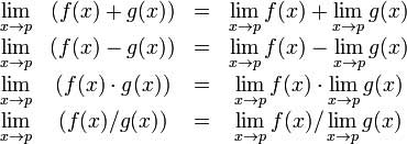
Let us consider two functions −
- f(x) = (3x + 5)/(x — 3)
- g(x) = x2 + 1.
Let us calculate the limits of the functions as x tends to 5, of both functions and verify the basic properties of limits using these two functions and MATLAB.
Example
Create a script file and type the following code into it −
syms x f = (3*x + 5)/(x-3); g = x^2 + 1; l1 = limit(f, 4) l2 = limit (g, 4) lAdd = limit(f + g, 4) lSub = limit(f - g, 4) lMult = limit(f*g, 4) lDiv = limit (f/g, 4)
When you run the file, it displays −
l1 = 17 l2 = 17 lAdd = 34 lSub = 0 lMult = 289 lDiv = 1
Verification of Basic Properties of Limits using Octave
Following is Octave version of the above example using symbolic package, try to execute and compare the result −
pkg load symbolic
symbols
x = sym("x");
f = (3*x + 5)/(x-3);
g = x^2 + 1;
l1 = subs(f, x, 4)
l2 = subs (g, x, 4)
lAdd = subs (f+g, x, 4)
lSub = subs (f-g, x, 4)
lMult = subs (f*g, x, 4)
lDiv = subs (f/g, x, 4)
Octave will execute the above statement and return the following result −
l1 = 17.0 l2 = 17.0 lAdd = 34.0 lSub = 0.0 lMult = 289.0 lDiv = 1.0
Left and Right Sided Limits
When a function has a discontinuity for some particular value of the variable, the limit does not exist at that point. In other words, limits of a function f(x) has discontinuity at x = a, when the value of limit, as x approaches x from left side, does not equal the value of the limit as x approaches from right side.
This leads to the concept of left-handed and right-handed limits. A left-handed limit is defined as the limit as x -> a, from the left, i.e., x approaches a, for values of x < a. A right-handed limit is defined as the limit as x -> a, from the right, i.e., x approaches a, for values of x > a. When the left-handed limit and right-handed limit are not equal, the limit does not exist.
Let us consider a function −
f(x) = (x — 3)/|x — 3|
We will show that limx->3 f(x) does not exist. MATLAB helps us to establish this fact in two ways −
- By plotting the graph of the function and showing the discontinuity.
- By computing the limits and showing that both are different.
The left-handed and right-handed limits are computed by passing the character strings ‘left’ and ‘right’ to the limit command as the last argument.
Example
Create a script file and type the following code into it −
f = (x - 3)/abs(x-3); ezplot(f,[-1,5]) l = limit(f,x,3,'left') r = limit(f,x,3,'right')
When you run the file, MATLAB draws the following plot

After this following output is displayed −
l = -1 r = 1
MATLAB — Differential
MATLAB provides the diff command for computing symbolic derivatives. In its simplest form, you pass the function you want to differentiate to diff command as an argument.
For example, let us compute the derivative of the function f(t) = 3t2 + 2t-2
Example
Create a script file and type the following code into it −
syms t f = 3*t^2 + 2*t^(-2); diff(f)
When the above code is compiled and executed, it produces the following result −
ans = 6*t - 4/t^3
Following is Octave equivalent of the above calculation −
pkg load symbolic
symbols
t = sym("t");
f = 3*t^2 + 2*t^(-2);
differentiate(f,t)
Octave executes the code and returns the following result −
ans = -(4.0)*t^(-3.0)+(6.0)*t
Verification of Elementary Rules of Differentiation
Let us briefly state various equations or rules for differentiation of functions and verify these rules. For this purpose, we will write f'(x) for a first order derivative and f»(x) for a second order derivative.
Following are the rules for differentiation −
Rule 1
For any functions f and g and any real numbers a and b are the derivative of the function −
h(x) = af(x) + bg(x) with respect to x is given by −
h'(x) = af'(x) + bg'(x)
Rule 2
The sum and subtraction rules state that if f and g are two functions, f’ and g’ are their derivatives respectively, then,
(f + g)’ = f’ + g’
(f — g)’ = f’ — g’
Rule 3
The product rule states that if f and g are two functions, f’ and g’ are their derivatives respectively, then,
(f.g)’ = f’.g + g’.f
Rule 4
The quotient rule states that if f and g are two functions, f’ and g’ are their derivatives respectively, then,
(f/g)’ = (f’.g — g’.f)/g2
Rule 5
The polynomial or elementary power rule states that, if y = f(x) = xn, then f’ = n. x(n-1)
A direct outcome of this rule is that the derivative of any constant is zero, i.e., if y = k, any constant, then
f’ = 0
Rule 6
The chain rule states that, derivative of the function of a function h(x) = f(g(x)) with respect to x is,
h'(x)= f'(g(x)).g'(x)
Example
Create a script file and type the following code into it −
syms x syms t f = (x + 2)*(x^2 + 3) der1 = diff(f) f = (t^2 + 3)*(sqrt(t) + t^3) der2 = diff(f) f = (x^2 - 2*x + 1)*(3*x^3 - 5*x^2 + 2) der3 = diff(f) f = (2*x^2 + 3*x)/(x^3 + 1) der4 = diff(f) f = (x^2 + 1)^17 der5 = diff(f) f = (t^3 + 3* t^2 + 5*t -9)^(-6) der6 = diff(f)
When you run the file, MATLAB displays the following result −
f = (x^2 + 3)*(x + 2) der1 = 2*x*(x + 2) + x^2 + 3 f = (t^(1/2) + t^3)*(t^2 + 3) der2 = (t^2 + 3)*(3*t^2 + 1/(2*t^(1/2))) + 2*t*(t^(1/2) + t^3) f = (x^2 - 2*x + 1)*(3*x^3 - 5*x^2 + 2) der3 = (2*x - 2)*(3*x^3 - 5*x^2 + 2) - (- 9*x^2 + 10*x)*(x^2 - 2*x + 1) f = (2*x^2 + 3*x)/(x^3 + 1) der4 = (4*x + 3)/(x^3 + 1) - (3*x^2*(2*x^2 + 3*x))/(x^3 + 1)^2 f = (x^2 + 1)^17 der5 = 34*x*(x^2 + 1)^16 f = 1/(t^3 + 3*t^2 + 5*t - 9)^6 der6 = -(6*(3*t^2 + 6*t + 5))/(t^3 + 3*t^2 + 5*t - 9)^7
Following is Octave equivalent of the above calculation −
pkg load symbolic
symbols
x = sym("x");
t = sym("t");
f = (x + 2)*(x^2 + 3)
der1 = differentiate(f,x)
f = (t^2 + 3)*(t^(1/2) + t^3)
der2 = differentiate(f,t)
f = (x^2 - 2*x + 1)*(3*x^3 - 5*x^2 + 2)
der3 = differentiate(f,x)
f = (2*x^2 + 3*x)/(x^3 + 1)
der4 = differentiate(f,x)
f = (x^2 + 1)^17
der5 = differentiate(f,x)
f = (t^3 + 3* t^2 + 5*t -9)^(-6)
der6 = differentiate(f,t)
Octave executes the code and returns the following result −
f = (2.0+x)*(3.0+x^(2.0)) der1 = 3.0+x^(2.0)+(2.0)*(2.0+x)*x f = (t^(3.0)+sqrt(t))*(3.0+t^(2.0)) der2 = (2.0)*(t^(3.0)+sqrt(t))*t+((3.0)*t^(2.0)+(0.5)*t^(-0.5))*(3.0+t^(2.0)) f = (1.0+x^(2.0)-(2.0)*x)*(2.0-(5.0)*x^(2.0)+(3.0)*x^(3.0)) der3 = (-2.0+(2.0)*x)*(2.0-(5.0)*x^(2.0)+(3.0)*x^(3.0))+((9.0)*x^(2.0)-(10.0)*x)*(1.0+x^(2.0)-(2.0)*x) f = (1.0+x^(3.0))^(-1)*((2.0)*x^(2.0)+(3.0)*x) der4 = (1.0+x^(3.0))^(-1)*(3.0+(4.0)*x)-(3.0)*(1.0+x^(3.0))^(-2)*x^(2.0)*((2.0)*x^(2.0)+(3.0)*x) f = (1.0+x^(2.0))^(17.0) der5 = (34.0)*(1.0+x^(2.0))^(16.0)*x f = (-9.0+(3.0)*t^(2.0)+t^(3.0)+(5.0)*t)^(-6.0) der6 = -(6.0)*(-9.0+(3.0)*t^(2.0)+t^(3.0)+(5.0)*t)^(-7.0)*(5.0+(3.0)*t^(2.0)+(6.0)*t)
Derivatives of Exponential, Logarithmic and Trigonometric Functions
The following table provides the derivatives of commonly used exponential, logarithmic and trigonometric functions −
| Function | Derivative |
|---|---|
| ca.x | ca.x.ln c.a (ln is natural logarithm) |
| ex | ex |
| ln x | 1/x |
| lncx | 1/x.ln c |
| xx | xx.(1 + ln x) |
| sin(x) | cos(x) |
| cos(x) | -sin(x) |
| tan(x) | sec2(x), or 1/cos2(x), or 1 + tan2(x) |
| cot(x) | -csc2(x), or -1/sin2(x), or -(1 + cot2(x)) |
| sec(x) | sec(x).tan(x) |
| csc(x) | -csc(x).cot(x) |
Example
Create a script file and type the following code into it −
syms x y = exp(x) diff(y) y = x^9 diff(y) y = sin(x) diff(y) y = tan(x) diff(y) y = cos(x) diff(y) y = log(x) diff(y) y = log10(x) diff(y) y = sin(x)^2 diff(y) y = cos(3*x^2 + 2*x + 1) diff(y) y = exp(x)/sin(x) diff(y)
When you run the file, MATLAB displays the following result −
y = exp(x) ans = exp(x) y = x^9 ans = 9*x^8 y = sin(x) ans = cos(x) y = tan(x) ans = tan(x)^2 + 1 y = cos(x) ans = -sin(x) y = log(x) ans = 1/x y = log(x)/log(10) ans = 1/(x*log(10)) y = sin(x)^2 ans = 2*cos(x)*sin(x) y = cos(3*x^2 + 2*x + 1) ans = -sin(3*x^2 + 2*x + 1)*(6*x + 2) y = exp(x)/sin(x) ans = exp(x)/sin(x) - (exp(x)*cos(x))/sin(x)^2
Following is Octave equivalent of the above calculation −
pkg load symbolic
symbols
x = sym("x");
y = Exp(x)
differentiate(y,x)
y = x^9
differentiate(y,x)
y = Sin(x)
differentiate(y,x)
y = Tan(x)
differentiate(y,x)
y = Cos(x)
differentiate(y,x)
y = Log(x)
differentiate(y,x)
% symbolic packages does not have this support
%y = Log10(x)
%differentiate(y,x)
y = Sin(x)^2
differentiate(y,x)
y = Cos(3*x^2 + 2*x + 1)
differentiate(y,x)
y = Exp(x)/Sin(x)
differentiate(y,x)
Octave executes the code and returns the following result −
y = exp(x) ans = exp(x) y = x^(9.0) ans = (9.0)*x^(8.0) y = sin(x) ans = cos(x) y = tan(x) ans = 1+tan(x)^2 y = cos(x) ans = -sin(x) y = log(x) ans = x^(-1) y = sin(x)^(2.0) ans = (2.0)*sin(x)*cos(x) y = cos(1.0+(2.0)*x+(3.0)*x^(2.0)) ans = -(2.0+(6.0)*x)*sin(1.0+(2.0)*x+(3.0)*x^(2.0)) y = sin(x)^(-1)*exp(x) ans = sin(x)^(-1)*exp(x)-sin(x)^(-2)*cos(x)*exp(x)
Computing Higher Order Derivatives
To compute higher derivatives of a function f, we use the syntax diff(f,n).
Let us compute the second derivative of the function y = f(x) = x .e-3x
f = x*exp(-3*x); diff(f, 2)
MATLAB executes the code and returns the following result −
ans = 9*x*exp(-3*x) - 6*exp(-3*x)
Following is Octave equivalent of the above calculation −
pkg load symbolic
symbols
x = sym("x");
f = x*Exp(-3*x);
differentiate(f, x, 2)
Octave executes the code and returns the following result −
ans = (9.0)*exp(-(3.0)*x)*x-(6.0)*exp(-(3.0)*x)
Example
In this example, let us solve a problem. Given that a function y = f(x) = 3 sin(x) + 7 cos(5x). We will have to find out whether the equation f» + f = -5cos(2x) holds true.
Create a script file and type the following code into it −
syms x
y = 3*sin(x)+7*cos(5*x); % defining the function
lhs = diff(y,2)+y; %evaluting the lhs of the equation
rhs = -5*cos(2*x); %rhs of the equation
if(isequal(lhs,rhs))
disp('Yes, the equation holds true');
else
disp('No, the equation does not hold true');
end
disp('Value of LHS is: '), disp(lhs);
When you run the file, it displays the following result −
No, the equation does not hold true Value of LHS is: -168*cos(5*x)
Following is Octave equivalent of the above calculation −
pkg load symbolic
symbols
x = sym("x");
y = 3*Sin(x)+7*Cos(5*x); % defining the function
lhs = differentiate(y, x, 2) + y; %evaluting the lhs of the equation
rhs = -5*Cos(2*x); %rhs of the equation
if(lhs == rhs)
disp('Yes, the equation holds true');
else
disp('No, the equation does not hold true');
end
disp('Value of LHS is: '), disp(lhs);
Octave executes the code and returns the following result −
No, the equation does not hold true Value of LHS is: -(168.0)*cos((5.0)*x)
Finding the Maxima and Minima of a Curve
If we are searching for the local maxima and minima for a graph, we are basically looking for the highest or lowest points on the graph of the function at a particular locality, or for a particular range of values of the symbolic variable.
For a function y = f(x) the points on the graph where the graph has zero slope are called stationary points. In other words stationary points are where f'(x) = 0.
To find the stationary points of a function we differentiate, we need to set the derivative equal to zero and solve the equation.
Example
Let us find the stationary points of the function f(x) = 2x3 + 3x2 − 12x + 17
Take the following steps −
First let us enter the function and plot its graph.
syms x y = 2*x^3 + 3*x^2 - 12*x + 17; % defining the function ezplot(y)
MATLAB executes the code and returns the following plot −
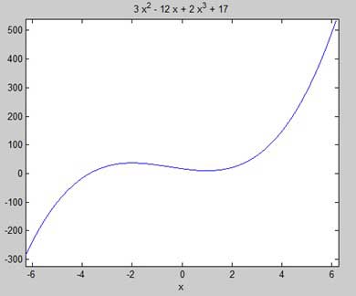
Here is Octave equivalent code for the above example −
pkg load symbolic
symbols
x = sym('x');
y = inline("2*x^3 + 3*x^2 - 12*x + 17");
ezplot(y)
print -deps graph.eps
Our aim is to find some local maxima and minima on the graph, so let us find the local maxima and minima for the interval [-2, 2] on the graph.
syms x y = 2*x^3 + 3*x^2 - 12*x + 17; % defining the function ezplot(y, [-2, 2])
MATLAB executes the code and returns the following plot −

Here is Octave equivalent code for the above example −
pkg load symbolic
symbols
x = sym('x');
y = inline("2*x^3 + 3*x^2 - 12*x + 17");
ezplot(y, [-2, 2])
print -deps graph.eps
Next, let us compute the derivative.
g = diff(y)
MATLAB executes the code and returns the following result −
g = 6*x^2 + 6*x - 12
Here is Octave equivalent of the above calculation −
pkg load symbolic
symbols
x = sym("x");
y = 2*x^3 + 3*x^2 - 12*x + 17;
g = differentiate(y,x)
Octave executes the code and returns the following result −
g = -12.0+(6.0)*x+(6.0)*x^(2.0)
Let us solve the derivative function, g, to get the values where it becomes zero.
s = solve(g)
MATLAB executes the code and returns the following result −
s = 1 -2
Following is Octave equivalent of the above calculation −
pkg load symbolic
symbols
x = sym("x");
y = 2*x^3 + 3*x^2 - 12*x + 17;
g = differentiate(y,x)
roots([6, 6, -12])
Octave executes the code and returns the following result −
g = -12.0+(6.0)*x^(2.0)+(6.0)*x ans = -2 1
This agrees with our plot. So let us evaluate the function f at the critical points x = 1, -2. We can substitute a value in a symbolic function by using the subs command.
subs(y, 1), subs(y, -2)
MATLAB executes the code and returns the following result −
ans = 10 ans = 37
Following is Octave equivalent of the above calculation −
pkg load symbolic
symbols
x = sym("x");
y = 2*x^3 + 3*x^2 - 12*x + 17;
g = differentiate(y,x)
roots([6, 6, -12])
subs(y, x, 1), subs(y, x, -2)
ans = 10.0 ans = 37.0-4.6734207789940138748E-18*I
Therefore, The minimum and maximum values on the function f(x) = 2x3 + 3x2 − 12x + 17, in the interval [-2,2] are 10 and 37.
Solving Differential Equations
MATLAB provides the dsolve command for solving differential equations symbolically.
The most basic form of the dsolve command for finding the solution to a single equation is
dsolve('eqn')
where eqn is a text string used to enter the equation.
It returns a symbolic solution with a set of arbitrary constants that MATLAB labels C1, C2, and so on.
You can also specify initial and boundary conditions for the problem, as comma-delimited list following the equation as −
dsolve('eqn','cond1', 'cond2',…)
For the purpose of using dsolve command, derivatives are indicated with a D. For example, an equation like f'(t) = -2*f + cost(t) is entered as −
‘Df = -2*f + cos(t)’
Higher derivatives are indicated by following D by the order of the derivative.
For example the equation f»(x) + 2f'(x) = 5sin3x should be entered as −
‘D2y + 2Dy = 5*sin(3*x)’
Let us take up a simple example of a first order differential equation: y’ = 5y.
s = dsolve('Dy = 5*y')
MATLAB executes the code and returns the following result −
s = C2*exp(5*t)
Let us take up another example of a second order differential equation as: y» — y = 0, y(0) = -1, y'(0) = 2.
dsolve('D2y - y = 0','y(0) = -1','Dy(0) = 2')
MATLAB executes the code and returns the following result −
ans = exp(t)/2 - (3*exp(-t))/2
MATLAB — Integration
Integration deals with two essentially different types of problems.
-
In the first type, derivative of a function is given and we want to find the function. Therefore, we basically reverse the process of differentiation. This reverse process is known as anti-differentiation, or finding the primitive function, or finding an indefinite integral.
-
The second type of problems involve adding up a very large number of very small quantities and then taking a limit as the size of the quantities approaches zero, while the number of terms tend to infinity. This process leads to the definition of the definite integral.
Definite integrals are used for finding area, volume, center of gravity, moment of inertia, work done by a force, and in numerous other applications.
Finding Indefinite Integral Using MATLAB
By definition, if the derivative of a function f(x) is f'(x), then we say that an indefinite integral of f'(x) with respect to x is f(x). For example, since the derivative (with respect to x) of x2 is 2x, we can say that an indefinite integral of 2x is x2.
In symbols −
f'(x2) = 2x, therefore,
∫ 2xdx = x2.
Indefinite integral is not unique, because derivative of x2 + c, for any value of a constant c, will also be 2x.
This is expressed in symbols as −
∫ 2xdx = x2 + c.
Where, c is called an ‘arbitrary constant’.
MATLAB provides an int command for calculating integral of an expression. To derive an expression for the indefinite integral of a function, we write −
int(f);
For example, from our previous example −
syms x int(2*x)
MATLAB executes the above statement and returns the following result −
ans = x^2
Example 1
In this example, let us find the integral of some commonly used expressions. Create a script file and type the following code in it −
syms x n int(sym(x^n)) f = 'sin(n*t)' int(sym(f)) syms a t int(a*cos(pi*t)) int(a^x)
When you run the file, it displays the following result −
ans = piecewise([n == -1, log(x)], [n ~= -1, x^(n + 1)/(n + 1)]) f = sin(n*t) ans = -cos(n*t)/n ans = (a*sin(pi*t))/pi ans = a^x/log(a)
Example 2
Create a script file and type the following code in it −
syms x n int(cos(x)) int(exp(x)) int(log(x)) int(x^-1) int(x^5*cos(5*x)) pretty(int(x^5*cos(5*x))) int(x^-5) int(sec(x)^2) pretty(int(1 - 10*x + 9 * x^2)) int((3 + 5*x -6*x^2 - 7*x^3)/2*x^2) pretty(int((3 + 5*x -6*x^2 - 7*x^3)/2*x^2))
Note that the pretty function returns an expression in a more readable format.
When you run the file, it displays the following result −
ans =
sin(x)
ans =
exp(x)
ans =
x*(log(x) - 1)
ans =
log(x)
ans =
(24*cos(5*x))/3125 + (24*x*sin(5*x))/625 - (12*x^2*cos(5*x))/125 + (x^4*cos(5*x))/5 - (4*x^3*sin(5*x))/25 + (x^5*sin(5*x))/5
2 4
24 cos(5 x) 24 x sin(5 x) 12 x cos(5 x) x cos(5 x)
----------- + ------------- - -------------- + ------------
3125 625 125 5
3 5
4 x sin(5 x) x sin(5 x)
------------- + -----------
25 5
ans =
-1/(4*x^4)
ans =
tan(x)
2
x (3 x - 5 x + 1)
ans =
- (7*x^6)/12 - (3*x^5)/5 + (5*x^4)/8 + x^3/2
6 5 4 3
7 x 3 x 5 x x
- ---- - ---- + ---- + --
12 5 8 2
Finding Definite Integral Using MATLAB
By definition, definite integral is basically the limit of a sum. We use definite integrals to find areas such as the area between a curve and the x-axis and the area between two curves. Definite integrals can also be used in other situations, where the quantity required can be expressed as the limit of a sum.
The int function can be used for definite integration by passing the limits over which you want to calculate the integral.
To calculate
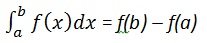
we write,
int(x, a, b)
For example, to calculate the value of  we write −
int(x, 4, 9)
MATLAB executes the above statement and returns the following result −
ans = 65/2
Following is Octave equivalent of the above calculation −
pkg load symbolic
symbols
x = sym("x");
f = x;
c = [1, 0];
integral = polyint(c);
a = polyval(integral, 9) - polyval(integral, 4);
display('Area: '), disp(double(a));
Octave executes the code and returns the following result −
Area: 32.500
An alternative solution can be given using quad() function provided by Octave as follows −
pkg load symbolic
symbols
f = inline("x");
[a, ierror, nfneval] = quad(f, 4, 9);
display('Area: '), disp(double(a));
Octave executes the code and returns the following result −
Area: 32.500
Example 1
Let us calculate the area enclosed between the x-axis, and the curve y = x3−2x+5 and the ordinates x = 1 and x = 2.
The required area is given by −
Create a script file and type the following code −
f = x^3 - 2*x +5;
a = int(f, 1, 2)
display('Area: '), disp(double(a));
When you run the file, it displays the following result −
a = 23/4 Area: 5.7500
Following is Octave equivalent of the above calculation −
pkg load symbolic
symbols
x = sym("x");
f = x^3 - 2*x +5;
c = [1, 0, -2, 5];
integral = polyint(c);
a = polyval(integral, 2) - polyval(integral, 1);
display('Area: '), disp(double(a));
Octave executes the code and returns the following result −
Area: 5.7500
An alternative solution can be given using quad() function provided by Octave as follows −
pkg load symbolic
symbols
x = sym("x");
f = inline("x^3 - 2*x +5");
[a, ierror, nfneval] = quad(f, 1, 2);
display('Area: '), disp(double(a));
Octave executes the code and returns the following result −
Area: 5.7500
Example 2
Find the area under the curve: f(x) = x2 cos(x) for −4 ≤ x ≤ 9.
Create a script file and write the following code −
f = x^2*cos(x);
ezplot(f, [-4,9])
a = int(f, -4, 9)
disp('Area: '), disp(double(a));
When you run the file, MATLAB plots the graph −

The output is given below −
a = 8*cos(4) + 18*cos(9) + 14*sin(4) + 79*sin(9) Area: 0.3326
Following is Octave equivalent of the above calculation −
pkg load symbolic
symbols
x = sym("x");
f = inline("x^2*cos(x)");
ezplot(f, [-4,9])
print -deps graph.eps
[a, ierror, nfneval] = quad(f, -4, 9);
display('Area: '), disp(double(a));
MATLAB — Polynomials
MATLAB represents polynomials as row vectors containing coefficients ordered by descending powers. For example, the equation P(x) = x4 + 7x3 — 5x + 9 could be represented as −
p = [1 7 0 -5 9];
Evaluating Polynomials
The polyval function is used for evaluating a polynomial at a specified value. For example, to evaluate our previous polynomial p, at x = 4, type −
p = [1 7 0 -5 9]; polyval(p,4)
MATLAB executes the above statements and returns the following result −
ans = 693
MATLAB also provides the polyvalm function for evaluating a matrix polynomial. A matrix polynomial is a polynomial with matrices as variables.
For example, let us create a square matrix X and evaluate the polynomial p, at X −
p = [1 7 0 -5 9]; X = [1 2 -3 4; 2 -5 6 3; 3 1 0 2; 5 -7 3 8]; polyvalm(p, X)
MATLAB executes the above statements and returns the following result −
ans =
2307 -1769 -939 4499
2314 -2376 -249 4695
2256 -1892 -549 4310
4570 -4532 -1062 9269
Finding the Roots of Polynomials
The roots function calculates the roots of a polynomial. For example, to calculate the roots of our polynomial p, type −
p = [1 7 0 -5 9]; r = roots(p)
MATLAB executes the above statements and returns the following result −
r = -6.8661 + 0.0000i -1.4247 + 0.0000i 0.6454 + 0.7095i 0.6454 - 0.7095i
The function poly is an inverse of the roots function and returns to the polynomial coefficients. For example −
p2 = poly(r)
MATLAB executes the above statements and returns the following result −
p2 =
Columns 1 through 3:
1.00000 + 0.00000i 7.00000 + 0.00000i 0.00000 + 0.00000i
Columns 4 and 5:
-5.00000 - 0.00000i 9.00000 + 0.00000i
Polynomial Curve Fitting
The polyfit function finds the coefficients of a polynomial that fits a set of data in a least-squares sense. If x and y are two vectors containing the x and y data to be fitted to a n-degree polynomial, then we get the polynomial fitting the data by writing −
p = polyfit(x,y,n)
Example
Create a script file and type the following code −
x = [1 2 3 4 5 6]; y = [5.5 43.1 128 290.7 498.4 978.67]; %data p = polyfit(x,y,4) %get the polynomial % Compute the values of the polyfit estimate over a finer range, % and plot the estimate over the real data values for comparison: x2 = 1:.1:6; y2 = polyval(p,x2); plot(x,y,'o',x2,y2) grid on
When you run the file, MATLAB displays the following result −
p = 4.1056 -47.9607 222.2598 -362.7453 191.1250
And plots the following graph −
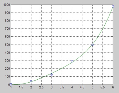
MATLAB — Transforms
MATLAB provides command for working with transforms, such as the Laplace and Fourier transforms. Transforms are used in science and engineering as a tool for simplifying analysis and look at data from another angle.
For example, the Fourier transform allows us to convert a signal represented as a function of time to a function of frequency. Laplace transform allows us to convert a differential equation to an algebraic equation.
MATLAB provides the laplace, fourier and fft commands to work with Laplace, Fourier and Fast Fourier transforms.
The Laplace Transform
The Laplace transform of a function of time f(t) is given by the following integral −
Laplace transform is also denoted as transform of f(t) to F(s). You can see this transform or integration process converts f(t), a function of the symbolic variable t, into another function F(s), with another variable s.
Laplace transform turns differential equations into algebraic ones. To compute a Laplace transform of a function f(t), write −
laplace(f(t))
Example
In this example, we will compute the Laplace transform of some commonly used functions.
Create a script file and type the following code −
syms s t a b w laplace(a) laplace(t^2) laplace(t^9) laplace(exp(-b*t)) laplace(sin(w*t)) laplace(cos(w*t))
When you run the file, it displays the following result −
ans = 1/s^2 ans = 2/s^3 ans = 362880/s^10 ans = 1/(b + s) ans = w/(s^2 + w^2) ans = s/(s^2 + w^2)
The Inverse Laplace Transform
MATLAB allows us to compute the inverse Laplace transform using the command ilaplace.
For example,
ilaplace(1/s^3)
MATLAB will execute the above statement and display the result −
ans = t^2/2
Example
Create a script file and type the following code −
syms s t a b w ilaplace(1/s^7) ilaplace(2/(w+s)) ilaplace(s/(s^2+4)) ilaplace(exp(-b*t)) ilaplace(w/(s^2 + w^2)) ilaplace(s/(s^2 + w^2))
When you run the file, it displays the following result −
ans = t^6/720 ans = 2*exp(-t*w) ans = cos(2*t) ans = ilaplace(exp(-b*t), t, x) ans = sin(t*w) ans = cos(t*w)
The Fourier Transforms
Fourier transforms commonly transforms a mathematical function of time, f(t), into a new function, sometimes denoted by or F, whose argument is frequency with units of cycles/s (hertz) or radians per second. The new function is then known as the Fourier transform and/or the frequency spectrum of the function f.
Example
Create a script file and type the following code in it −
syms x f = exp(-2*x^2); %our function ezplot(f,[-2,2]) % plot of our function FT = fourier(f) % Fourier transform
When you run the file, MATLAB plots the following graph −

The following result is displayed −
FT = (2^(1/2)*pi^(1/2)*exp(-w^2/8))/2
Plotting the Fourier transform as −
ezplot(FT)
Gives the following graph −
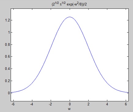
Inverse Fourier Transforms
MATLAB provides the ifourier command for computing the inverse Fourier transform of a function. For example,
f = ifourier(-2*exp(-abs(w)))
MATLAB will execute the above statement and display the result −
f = -2/(pi*(x^2 + 1))
MATLAB — GNU Octave Tutorial
GNU Octave is a high-level programming language like MATLAB and it is mostly compatible with MATLAB. It is also used for numerical computations.
Octave has the following common features with MATLAB −
- matrices are fundamental data type
- it has built-in support for complex numbers
- it has built-in math functions and libraries
- it supports user-defined functions
GNU Octave is also freely redistributable software. You may redistribute it and/or modify it under the terms of the GNU General Public License (GPL) as published by the Free Software Foundation.
MATLAB vs Octave
Most MATLAB programs run in Octave, but some of the Octave programs may not run in MATLAB because, Octave allows some syntax that MATLAB does not.
For example, MATLAB supports single quotes only, but Octave supports both single and double quotes for defining strings. If you are looking for a tutorial on Octave, then kindly go through this tutorial from beginning which covers both MATLAB as well as Octave.
Compatible Examples
Almost all the examples covered in this tutorial are compatible with MATLAB as well as Octave. Let’s try following example in MATLAB and Octave which produces same result without any syntax changes −
This example creates a 3D surface map for the function g = xe-(x2 + y2). Create a script file and type the following code −
[x,y] = meshgrid(-2:.2:2); g = x .* exp(-x.^2 - y.^2); surf(x, y, g) print -deps graph.eps
When you run the file, MATLAB displays the following 3-D map −
Non-compatible Examples
Though all the core functionality of MATLAB is available in Octave, there are some functionality for example, Differential & Integration Calculus, which does not match exactly in both the languages. This tutorial has tried to give both type of examples where they differed in their syntax.
Consider following example where MATLAB and Octave make use of different functions to get the area of a curve: f(x) = x2 cos(x) for −4 ≤ x ≤ 9. Following is MATLAB version of the code −
f = x^2*cos(x);
ezplot(f, [-4,9])
a = int(f, -4, 9)
disp('Area: '), disp(double(a));
When you run the file, MATLAB plots the graph −
The following result is displayed
a = 8*cos(4) + 18*cos(9) + 14*sin(4) + 79*sin(9) Area: 0.3326
But to give area of the same curve in Octave, you will have to make use of symbolic package as follows −
pkg load symbolic
symbols
x = sym("x");
f = inline("x^2*cos(x)");
ezplot(f, [-4,9])
print -deps graph.eps
[a, ierror, nfneval] = quad(f, -4, 9);
display('Area: '), disp(double(a));
MATLAB — Simulink
Simulink is a simulation and model-based design environment for dynamic and embedded systems, integrated with MATLAB. Simulink, also developed by MathWorks, is a data flow graphical programming language tool for modelling, simulating and analyzing multi-domain dynamic systems. It is basically a graphical block diagramming tool with customizable set of block libraries.
It allows you to incorporate MATLAB algorithms into models as well as export the simulation results into MATLAB for further analysis.
Simulink supports −
- system-level design
- simulation
- automatic code generation
- testing and verification of embedded systems
There are several other add-on products provided by MathWorks and third-party hardware and software products that are available for use with Simulink.
The following list gives brief description of some of them −
-
Stateflow allows developing state machines and flow charts.
-
Simulink Coder allows the generation of C source code for real-time implementation of systems automatically.
-
xPC Target together with x86-based real-time systems provide an environment to simulate and test Simulink and Stateflow models in real-time on the physical system.
-
Embedded Coder supports specific embedded targets.
-
HDL Coder allows to automatically generate synthesizable VHDL and Verilog.
-
SimEvents provides a library of graphical building blocks for modelling queuing systems.
Simulink is capable of systematic verification and validation of models through modelling style checking, requirements traceability and model coverage analysis.
Simulink Design Verifier allows you to identify design errors and to generate test case scenarios for model checking.
Using Simulink
To open Simulink, type in the MATLAB work space −
simulink
Simulink opens with the Library Browser. The Library Browser is used for building simulation models.
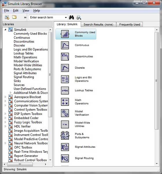
On the left side window pane, you will find several libraries categorized on the basis of various systems, clicking on each one will display the design blocks on the right window pane.
Building Models
To create a new model, click the New button on the Library Browser’s toolbar. This opens a new untitled model window.
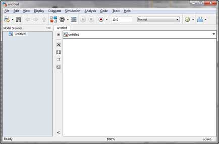
A Simulink model is a block diagram.
Model elements are added by selecting the appropriate elements from the Library Browser and dragging them into the Model window.
Alternately, you can copy the model elements and paste them into the model window.
Examples
Drag and drop items from the Simulink library to make your project.
For the purpose of this example, two blocks will be used for the simulation — A Source (a signal) and a Sink (a scope). A signal generator (the source) generates an analog signal, which will then be graphically visualized by the scope(the sink).

Begin by dragging the required blocks from the library to the project window. Then, connect the blocks together which can be done by dragging connectors from connection points on one block to those of another.
Let us drag a ‘Sine Wave’ block into the model.
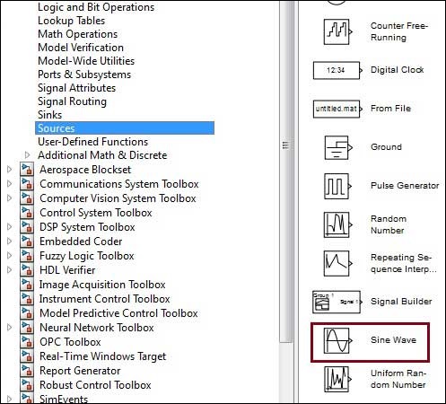
Select ‘Sinks’ from the library and drag a ‘Scope’ block into the model.

Drag a signal line from the output of the Sine Wave block to the input of the Scope block.
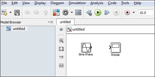

Run the simulation by pressing the ‘Run‘ button, keeping all parameters default (you can change them from the Simulation menu)
You should get the below graph from the scope.
©
Евгений Михайлов, Алексей Померанцев
Российское
хемометрическое общество http://rcs.chph.ras.ru/
Содержание
Введение
1.
Базовые сведения
1.1.
Рабочая среда MatLab
1.2.
Простейшие вычисления
1.3.
Эхо команд
1.4.
Сохранение рабочей среды. MAT файлы
1.5.
Журнал
1.6.
Система помощи
2.
Матрицы
2.1.
Скаляры, векторы и матрицы
2.2.
Доступ к элементам
2.3
Основные матричные операции
2.4.
Создание матриц специального вида
2.5.
Матричные вычисления
3.
Интегрирование MatLab и Excel
3.1.
Конфигурирование Excel
3.2.
Обмен данными между MatLab и Excel
4.Программирование
4.1.
М-файлы
4.2.
Файл-программа
4.3.
Файл-функция
4.4.
Создание графика
4.5.
Печать графиков
5.
Примеры программ
5.1.
Центрирование и шкалирование
5.2.
SVD/PCA
5.3.
PCA/NIPALS
5.4.
PLS1
5.5.
PLS2
Заключение
Введение
В
этом пособии рассказывается о применении
пакета MatLab для
анализа многомерных данных. Этот текст
не является учебником по MatLab. В нем
приведены только базовые сведения
о работе в этой среде, необходимые для
реализации основных алгоритмов. Более
подробное изложение можно найти здесь.
В
пособии интенсивно используются понятия
и методы матричной алгебры – вектор,
матрица, и т.п. Читателям, которые плохо
знакомы с этим аппаратом, рекомендуется
изучить, или, хотя бы просмотреть, пособие
«Матрицы
и векторы«.
Для
практического воплощения хемометрических
методов используются как специализированные
пакеты программ (например, the
Unsrambler или SIMCA),
так и статистические пакеты общего
назначения (например, SPSS или Statistica).
Среди средств общего назначения,
используемых в хемометрике, особое
место занимает пакет MatLab. Его популярность
необычайно высока. Это объясняется тем,
что MatLab является мощным и универсальным
средством обработки многомерных данных.
Сама структура пакета делает его удобным
средством для проведения матричных
вычислений. Спектр проблем, исследование
которых может, осуществлено при помощи
MatLab, охватывает: матричный анализ,
обработку сигналов и изображений,
нейронные сети и многие другие. MatLab —
это язык высокого уровня, имеющий
открытый код, что дает возможность
опытным пользователям разбираться в
запрограммированных алгоритмах. Простой
встроенный язык программирования
позволяет легко создавать собственные
алгоритмы. За много лет использования
MatLab создано огромное количество функций
и ToolBox (пакетов специализированных
средств). Самым популярным является
пакет PLS
ToolBox компании Eigenvector
Research, Inc.
Многие книги
и статьи содержат MatLab коды, позволяющие
читателю сразу применить описываемые
методы на практике. MatLab прекрасно
интегрируется с Microsoft Word и Excel. Российское
хемометрическое общество издало учебное
пособие,
являющееся полезным введением в
хемометрические приложения MatLab.
Другие
материалы по той же теме:
-
Матрицы
и векторы -
Проекционные
методы в системе Excel. -
Калибровка
(Градуировка) -
Метод
главных компонент (PCA) -
Хемометрика
в аналитической химии -
Четвертая
парадигма -
Технология
анализа процессов (PAT) -
ПЛС-регрессия
и ковариация -
Методы
классификации
Содержание
Соседние файлы в папке MatLab
- #
- #
- #
- #
- #
- #
- #
В данном плейлисте рассмотрены основные аспекты по работе в среде MATLAB.
Список видео, входящих в плейлист «Введение в MATLAB»:
- Начало работы
- Среда разработки
- Написание программ
- Массивы и матрицы
- Фундаментальные классы (типы данных)
- Структуры и массивы ячеек
- Интерактивное построение графиков
- Расширенное построение графиков: особенности и приемы
01 Начало работы
Базовые функции MATLAB, переменные, команды, массивы, индексация массивов, матрицы и матричные операции, синтаксис языка, построение графиков, работа с командной строкой, всплывающие подсказки, справка.
Документация по теме «Начало работы с MATLAB»
02 Среда разработки
Работа с такими инструментами, как история команд, браузер рабочего пространства и редактор переменных, сохранение и загрузка данных в рабочее пространство, а также управление окнами и панелями рабочего стола MATLAB. Подробно показан интерфейс программы.
Документация по теме «Среда и настройки»
03 Написание программ
Написание программ MATLAB, включая создание скриптов и функций.
Документация по теме «Программирование»
04 Массивы и матрицы
Создание и манипуляции с массивами в MATLAB, включая доступ к элементам с использованием индексации.
Документация по теме «Матрицы в среде MATLAB»
05 Фундаментальные классы (типы данных)
Работа с численными, текстовыми и логическими типами данных в MATLAB.
Документация по теме «Типы данных»
06 Структуры и массивы ячеек
Использование структур и массивов ячеек в MATLAB для управления гетерогенными данными различных типов и размеров.
Документация по теме «Структуры» и «Массивы ячеек».
07 Интерактивное построение графиков
Интерактивное построение базовых графиков в среде разработки MATLAB.
Документация по теме «Графика»
08 Расширенное построение графиков: особенности и приемы
Создание графиков программным способом с использованием базовых функций для построения графиков в MATLAB.
Документация по теме «Графика»
Main Content
The Language of Technical Computing
Millions of engineers and scientists worldwide use MATLAB® to analyze and design the systems and products transforming our world. The
matrix-based MATLAB language is the world’s most natural way to express computational mathematics.
Built-in graphics make it easy to visualize and gain insights from data. The desktop
environment invites experimentation, exploration, and discovery. These MATLAB tools and capabilities are all rigorously tested and designed to work
together.
MATLAB helps you take your ideas beyond the desktop. You can run your analyses on
larger data sets, and scale up to clusters and clouds. MATLAB code can be integrated with other languages, enabling you to deploy algorithms
and applications within web, enterprise, and production systems.
Installation and Configuration
Tutorials
- Desktop Basics
Enter statements at the command line and view results.
- Matrices and Arrays
MATLAB operates primarily on arrays and matrices,
both in whole and in part. A matrix is a two-dimensional array often
used for linear algebra. - Array Indexing
Variables in MATLAB are typically arrays that
can hold many numbers. When you want to access selected elements of
an array, use indexing. - Workspace Variables
The workspace contains variables that you create within
or import into MATLAB from data files or other programs. - Text and Characters
Create string arrays for text, or create character arrays for data.
- Calling Functions
MATLAB provides a large number of functions that
perform computational tasks. To call a function, enclose its input
arguments in parentheses. - 2-D and 3-D Plots
Graphics functions include 2-D and 3-D plotting functions to visualize data
and communicate results. - Programming and Scripts
The simplest type of MATLAB program is called a script. A script contains a sequence of
commands and function calls. - Help and Documentation
All functions have supporting documentation that includes examples and
describes the function inputs, outputs, and calling syntax.