Note
Click here
to download the full example code
This tutorial covers some basic usage patterns and best practices to
help you get started with Matplotlib.
import matplotlib as mpl
import matplotlib.pyplot as plt
import numpy as np
A simple example#
Matplotlib graphs your data on Figures (e.g., windows, Jupyter
widgets, etc.), each of which can contain one or more Axes, an
area where points can be specified in terms of x-y coordinates (or theta-r
in a polar plot, x-y-z in a 3D plot, etc.). The simplest way of
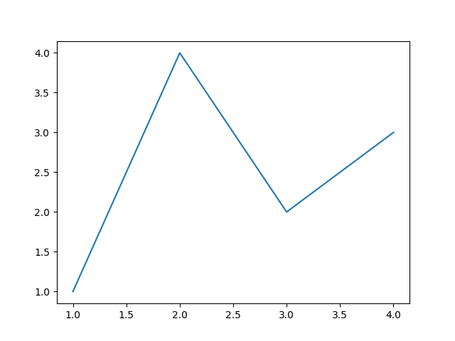
creating a Figure with an Axes is using pyplot.subplots. We can then use
Axes.plot to draw some data on the Axes:
fig, ax = plt.subplots()  # Create a figure containing a single axes.
ax.plot([1, 2, 3, 4], [1, 4, 2, 3])  # Plot some data on the axes.
Note that to get this Figure to display, you may have to call plt.show(),
depending on your backend. For more details of Figures and backends, see
Creating, viewing, and saving Matplotlib Figures.
Parts of a Figure#
Here are the components of a Matplotlib Figure.

Figure#
The whole figure. The Figure keeps
track of all the child Axes, a group of
‘special’ Artists (titles, figure legends, colorbars, etc), and
even nested subfigures.
The easiest way to create a new Figure is with pyplot:
It is often convenient to create the Axes together with the Figure, but you
can also manually add Axes later on. Note that many
Matplotlib backends support zooming and
panning on figure windows.
For more on Figures, see Creating, viewing, and saving Matplotlib Figures.
Axes#
An Axes is an Artist attached to a Figure that contains a region for
plotting data, and usually includes two (or three in the case of 3D)
Axis objects (be aware of the difference
between Axes and Axis) that provide ticks and tick labels to
provide scales for the data in the Axes. Each Axes also
has a title
(set via set_title()), an x-label (set via
set_xlabel()), and a y-label set via
set_ylabel()).
The Axes class and its member functions are the primary
entry point to working with the OOP interface, and have most of the
plotting methods defined on them (e.g. ax.plot(), shown above, uses
the plot method)
Axis#
These objects set the scale and limits and generate ticks (the marks
on the Axis) and ticklabels (strings labeling the ticks). The location
of the ticks is determined by a Locator object and the
ticklabel strings are formatted by a Formatter. The
combination of the correct Locator and Formatter gives very fine
control over the tick locations and labels.
Artist#
Basically, everything visible on the Figure is an Artist (even
Figure, Axes, and Axis objects). This includes
Text objects, Line2D objects, collections objects, Patch
objects, etc. When the Figure is rendered, all of the
Artists are drawn to the canvas. Most Artists are tied to an Axes; such
an Artist cannot be shared by multiple Axes, or moved from one to another.
Types of inputs to plotting functions#
Plotting functions expect numpy.array or numpy.ma.masked_array as
input, or objects that can be passed to numpy.asarray.
Classes that are similar to arrays (‘array-like’) such as pandas
data objects and numpy.matrix may not work as intended. Common convention
is to convert these to numpy.array objects prior to plotting.
For example, to convert a numpy.matrix
b = np.matrix([[1, 2], [3, 4]])
b_asarray = np.asarray(b)
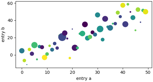
Most methods will also parse an addressable object like a dict, a
numpy.recarray, or a pandas.DataFrame. Matplotlib allows you to
provide the data keyword argument and generate plots passing the
strings corresponding to the x and y variables.
np.random.seed(19680801)  # seed the random number generator.
data = {'a': np.arange(50),
        'c': np.random.randint(0, 50, 50),
        'd': np.random.randn(50)}
data['b'] = data['a'] + 10 * np.random.randn(50)
data['d'] = np.abs(data['d']) * 100

fig, ax = plt.subplots(figsize=(5, 2.7), layout='constrained')
ax.scatter('a', 'b', c='c', s='d', data=data)
ax.set_xlabel('entry a')
ax.set_ylabel('entry b')
Coding styles#
The explicit and the implicit interfaces#
As noted above, there are essentially two ways to use Matplotlib:
-
Explicitly create Figures and Axes, and call methods on them (the
«object-oriented (OO) style»). -
Rely on pyplot to implicitly create and manage the Figures and Axes, and
use pyplot functions for plotting.
See Matplotlib Application Interfaces (APIs) for an explanation of the tradeoffs between the
implicit and explicit interfaces.
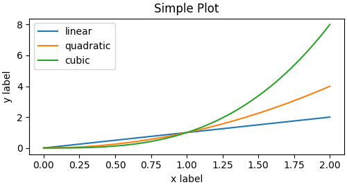
So one can use the OO-style
x = np.linspace(0, 2, 100)  # Sample data.

# Note that even in the OO-style, we use `.pyplot.figure` to create the Figure.
fig, ax = plt.subplots(figsize=(5, 2.7), layout='constrained')
ax.plot(x, x, label='linear')  # Plot some data on the axes.
ax.plot(x, x**2, label='quadratic')  # Plot more data on the axes...
ax.plot(x, x**3, label='cubic')  # ... and some more.
ax.set_xlabel('x label')  # Add an x-label to the axes.
ax.set_ylabel('y label')  # Add a y-label to the axes.
ax.set_title("Simple Plot")  # Add a title to the axes.
ax.legend()  # Add a legend.

or the pyplot-style:
x = np.linspace(0, 2, 100)  # Sample data.

plt.figure(figsize=(5, 2.7), layout='constrained')
plt.plot(x, x, label='linear')  # Plot some data on the (implicit) axes.
plt.plot(x, x**2, label='quadratic')  # etc.
plt.plot(x, x**3, label='cubic')
plt.xlabel('x label')
plt.ylabel('y label')
plt.title("Simple Plot")
plt.legend()
(In addition, there is a third approach, for the case when embedding
Matplotlib in a GUI application, which completely drops pyplot, even for
figure creation. See the corresponding section in the gallery for more info:
Embedding Matplotlib in graphical user interfaces.)
Matplotlib’s documentation and examples use both the OO and the pyplot
styles. In general, we suggest using the OO style, particularly for
complicated plots, and functions and scripts that are intended to be reused
as part of a larger project. However, the pyplot style can be very convenient
for quick interactive work.
Note
You may find older examples that use the pylab interface,
via from pylab import *. This approach is strongly deprecated.
Making a helper functions#
If you need to make the same plots over and over again with different data
sets, or want to easily wrap Matplotlib methods, use the recommended
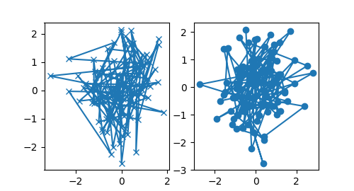
signature function below.
which you would then use twice to populate two subplots:
data1, data2, data3, data4 = np.random.randn(4, 100)  # make 4 random data sets
fig, (ax1, ax2) = plt.subplots(1, 2, figsize=(5, 2.7))
my_plotter(ax1, data1, data2, {'marker': 'x'})
my_plotter(ax2, data3, data4, {'marker': 'o'})
Note that if you want to install these as a python package, or any other
customizations you could use one of the many templates on the web;
Matplotlib has one at mpl-cookiecutter
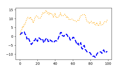
Styling Artists#
Most plotting methods have styling options for the Artists, accessible either
when a plotting method is called, or from a «setter» on the Artist. In the
plot below we manually set the color, linewidth, and linestyle of the
Artists created by plot, and we set the linestyle of the second line
after the fact with set_linestyle.
fig, ax = plt.subplots(figsize=(5, 2.7))
x = np.arange(len(data1))
ax.plot(x, np.cumsum(data1), color='blue', linewidth=3, linestyle='--')
l, = ax.plot(x, np.cumsum(data2), color='orange', linewidth=2)
l.set_linestyle(':')
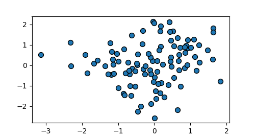
Colors#
Matplotlib has a very flexible array of colors that are accepted for most
Artists; see the colors tutorial for a
list of specifications. Some Artists will take multiple colors. i.e. for
a scatter plot, the edge of the markers can be different colors
from the interior:
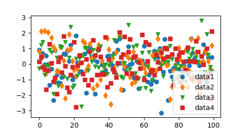
Linewidths, linestyles, and markersizes#
Line widths are typically in typographic points (1 pt = 1/72 inch) and
available for Artists that have stroked lines. Similarly, stroked lines
can have a linestyle. See the linestyles example.
Marker size depends on the method being used. plot specifies
markersize in points, and is generally the «diameter» or width of the
marker. scatter specifies markersize as approximately
proportional to the visual area of the marker. There is an array of
markerstyles available as string codes (see markers), or
users can define their own MarkerStyle (see
Marker reference):
fig, ax = plt.subplots(figsize=(5, 2.7))
ax.plot(data1, 'o', label='data1')
ax.plot(data2, 'd', label='data2')
ax.plot(data3, 'v', label='data3')
ax.plot(data4, 's', label='data4')
ax.legend()
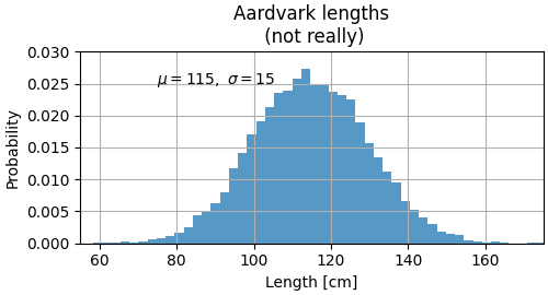
Labelling plots#
Axes labels and text#
set_xlabel, set_ylabel, and set_title are used to
add text in the indicated locations (see Text in Matplotlib Plots
for more discussion). Text can also be directly added to plots using
text:
mu, sigma = 115, 15
x = mu + sigma * np.random.randn(10000)
fig, ax = plt.subplots(figsize=(5, 2.7), layout='constrained')
# the histogram of the data
n, bins, patches = ax.hist(x, 50, density=True, facecolor='C0', alpha=0.75)

ax.set_xlabel('Length [cm]')
ax.set_ylabel('Probability')
ax.set_title('Aardvark lengthsn (not really)')
ax.text(75, .025, r'$mu=115, sigma=15$')
ax.axis([55, 175, 0, 0.03])
ax.grid(True)
All of the text functions return a matplotlib.text.Text
instance. Just as with lines above, you can customize the properties by
passing keyword arguments into the text functions:
These properties are covered in more detail in
Text properties and layout.
Using mathematical expressions in text#
Matplotlib accepts TeX equation expressions in any text expression.
For example to write the expression (sigma_i=15) in the title,
you can write a TeX expression surrounded by dollar signs:
where the r preceding the title string signifies that the string is a
raw string and not to treat backslashes as python escapes.
Matplotlib has a built-in TeX expression parser and
layout engine, and ships its own math fonts – for details see
Writing mathematical expressions. You can also use LaTeX directly to format
your text and incorporate the output directly into your display figures or
saved postscript – see Text rendering with LaTeX.
Annotations#
We can also annotate points on a plot, often by connecting an arrow pointing
to xy, to a piece of text at xytext:
fig, ax = plt.subplots(figsize=(5, 2.7))

t = np.arange(0.0, 5.0, 0.01)
s = np.cos(2 * np.pi * t)
line, = ax.plot(t, s, lw=2)

ax.annotate('local max', xy=(2, 1), xytext=(3, 1.5),
            arrowprops=dict(facecolor='black', shrink=0.05))

ax.set_ylim(-2, 2)
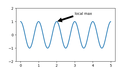
In this basic example, both xy and xytext are in data coordinates.
There are a variety of other coordinate systems one can choose — see
Basic annotation and Advanced annotation for
details. More examples also can be found in
Annotating Plots.
Axis scales and ticks#
Each Axes has two (or three) Axis objects representing the x- and
y-axis. These control the scale of the Axis, the tick locators and the
tick formatters. Additional Axes can be attached to display further Axis
objects.
Scales#
In addition to the linear scale, Matplotlib supplies non-linear scales,
such as a log-scale. Since log-scales are used so much there are also
direct methods like loglog, semilogx, and
semilogy. There are a number of scales (see
Scales for other examples). Here we set the scale
manually:
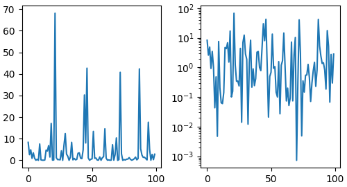
The scale sets the mapping from data values to spacing along the Axis. This
happens in both directions, and gets combined into a transform, which
is the way that Matplotlib maps from data coordinates to Axes, Figure, or
screen coordinates. See Transformations Tutorial.
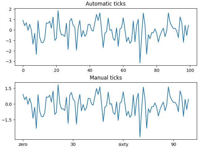
Tick locators and formatters#
Each Axis has a tick locator and formatter that choose where along the
Axis objects to put tick marks. A simple interface to this is
set_xticks:
fig, axs = plt.subplots(2, 1, layout='constrained')
axs[0].plot(xdata, data1)
axs[0].set_title('Automatic ticks')

axs[1].plot(xdata, data1)
axs[1].set_xticks(np.arange(0, 100, 30), ['zero', '30', 'sixty', '90'])
axs[1].set_yticks([-1.5, 0, 1.5])  # note that we don't need to specify labels
axs[1].set_title('Manual ticks')
Different scales can have different locators and formatters; for instance
the log-scale above uses LogLocator and LogFormatter. See
Tick locators and
Tick formatters for other formatters and
locators and information for writing your own.
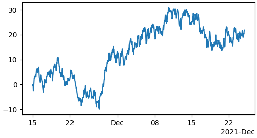
Plotting dates and strings#
Matplotlib can handle plotting arrays of dates and arrays of strings, as
well as floating point numbers. These get special locators and formatters
as appropriate. For dates:
For more information see the date examples
(e.g. Date tick labels)
For strings, we get categorical plotting (see:
Plotting categorical variables).
One caveat about categorical plotting is that some methods of parsing
text files return a list of strings, even if the strings all represent
numbers or dates. If you pass 1000 strings, Matplotlib will think you
meant 1000 categories and will add 1000 ticks to your plot!
Additional Axis objects#
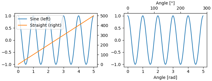
Plotting data of different magnitude in one chart may require
an additional y-axis. Such an Axis can be created by using
twinx to add a new Axes with an invisible x-axis and a y-axis
positioned at the right (analogously for twiny). See
Plots with different scales for another example.
Similarly, you can add a secondary_xaxis or
secondary_yaxis having a different scale than the main Axis to
represent the data in different scales or units. See
Secondary Axis for further
examples.
fig, (ax1, ax3) = plt.subplots(1, 2, figsize=(7, 2.7), layout='constrained')
l1, = ax1.plot(t, s)
ax2 = ax1.twinx()
l2, = ax2.plot(t, range(len(t)), 'C1')
ax2.legend([l1, l2], ['Sine (left)', 'Straight (right)'])

ax3.plot(t, s)
ax3.set_xlabel('Angle [rad]')
ax4 = ax3.secondary_xaxis('top', functions=(np.rad2deg, np.deg2rad))
ax4.set_xlabel('Angle [°]')
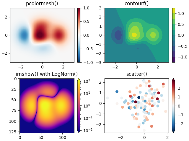
Color mapped data#
Often we want to have a third dimension in a plot represented by a colors in
a colormap. Matplotlib has a number of plot types that do this:
X, Y = np.meshgrid(np.linspace(-3, 3, 128), np.linspace(-3, 3, 128))
Z = (1 - X/2 + X**5 + Y**3) * np.exp(-X**2 - Y**2)

fig, axs = plt.subplots(2, 2, layout='constrained')
pc = axs[0, 0].pcolormesh(X, Y, Z, vmin=-1, vmax=1, cmap='RdBu_r')
fig.colorbar(pc, ax=axs[0, 0])
axs[0, 0].set_title('pcolormesh()')

co = axs[0, 1].contourf(X, Y, Z, levels=np.linspace(-1.25, 1.25, 11))
fig.colorbar(co, ax=axs[0, 1])
axs[0, 1].set_title('contourf()')

pc = axs[1, 0].imshow(Z**2 * 100, cmap='plasma',
                          norm=mpl.colors.LogNorm(vmin=0.01, vmax=100))
fig.colorbar(pc, ax=axs[1, 0], extend='both')
axs[1, 0].set_title('imshow() with LogNorm()')

pc = axs[1, 1].scatter(data1, data2, c=data3, cmap='RdBu_r')
fig.colorbar(pc, ax=axs[1, 1], extend='both')
axs[1, 1].set_title('scatter()')
Colormaps#
These are all examples of Artists that derive from ScalarMappable
objects. They all can set a linear mapping between vmin and vmax into
the colormap specified by cmap. Matplotlib has many colormaps to choose
from (Choosing Colormaps in Matplotlib) you can make your
own (Creating Colormaps in Matplotlib) or download as
third-party packages.
Normalizations#
Sometimes we want a non-linear mapping of the data to the colormap, as
in the LogNorm example above. We do this by supplying the
ScalarMappable with the norm argument instead of vmin and vmax.
More normalizations are shown at Colormap Normalization.
Colorbars#
Adding a colorbar gives a key to relate the color back to the
underlying data. Colorbars are figure-level Artists, and are attached to
a ScalarMappable (where they get their information about the norm and
colormap) and usually steal space from a parent Axes. Placement of
colorbars can be complex: see
Placing Colorbars for
details. You can also change the appearance of colorbars with the
extend keyword to add arrows to the ends, and shrink and aspect to
control the size. Finally, the colorbar will have default locators
and formatters appropriate to the norm. These can be changed as for
other Axis objects.
Working with multiple Figures and Axes#
You can open multiple Figures with multiple calls to
fig = plt.figure() or fig2, ax = plt.subplots(). By keeping the
object references you can add Artists to either Figure.
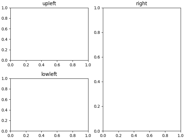
Multiple Axes can be added a number of ways, but the most basic is
plt.subplots() as used above. One can achieve more complex layouts,
with Axes objects spanning columns or rows, using subplot_mosaic.
fig, axd = plt.subplot_mosaic([['upleft', 'right'],
                               ['lowleft', 'right']], layout='constrained')
axd['upleft'].set_title('upleft')
axd['lowleft'].set_title('lowleft')
axd['right'].set_title('right')
Matplotlib has quite sophisticated tools for arranging Axes: See
Arranging multiple Axes in a Figure and
Complex and semantic figure composition (subplot_mosaic).
More reading#
For more plot types see Plot types and the
API reference, in particular the
Axes API.
Total running time of the script: ( 0 minutes 8.602 seconds)
Gallery generated by Sphinx-Gallery
#статьи
- 13 фев 2023
-

0
Разбираемся в том, как работает библиотека Matplotlib, и строим первые графики.
Иллюстрация: Оля Ежак для Skillbox Media

Изучает Python, его библиотеки и занимается анализом данных. Любит путешествовать в горах.
Matplotlib — популярная Python-библиотека для визуализации данных. Она используется для создания любых видов графиков: линейных, круговых диаграмм, построчных гистограмм и других — в зависимости от задач.
В этой статье научимся импортировать библиотеку и на примерах разберём основные способы визуализации данных.
Библиотека Matplotlib — пакет для визуализации данных в Python, который позволяет работать с данными на нескольких уровнях:
- с помощью модуля Pyplot, который рассматривает график как единое целое;
- через объектно-ориентированный интерфейс, когда каждая фигура или её часть является отдельным объектом, — это позволяет выборочно менять их свойства и отображение.
В этой статье мы будем работать с модулем Pyplot, которого достаточно для построения графиков.
Matplotlib используют для визуализации данных любой сложности. Библиотека позволяет строить разные варианты графиков: линейные, трёхмерные, диаграммы рассеяния и другие, а также комбинировать их.
Дополнительные библиотеки позволяют расширить возможности анализа данных. Например, модуль Cartopy добавляет возможность работать с картографической информацией. Подробно про Matplotlib можно узнать из официальной документации.
Инфографика: Matplotlib
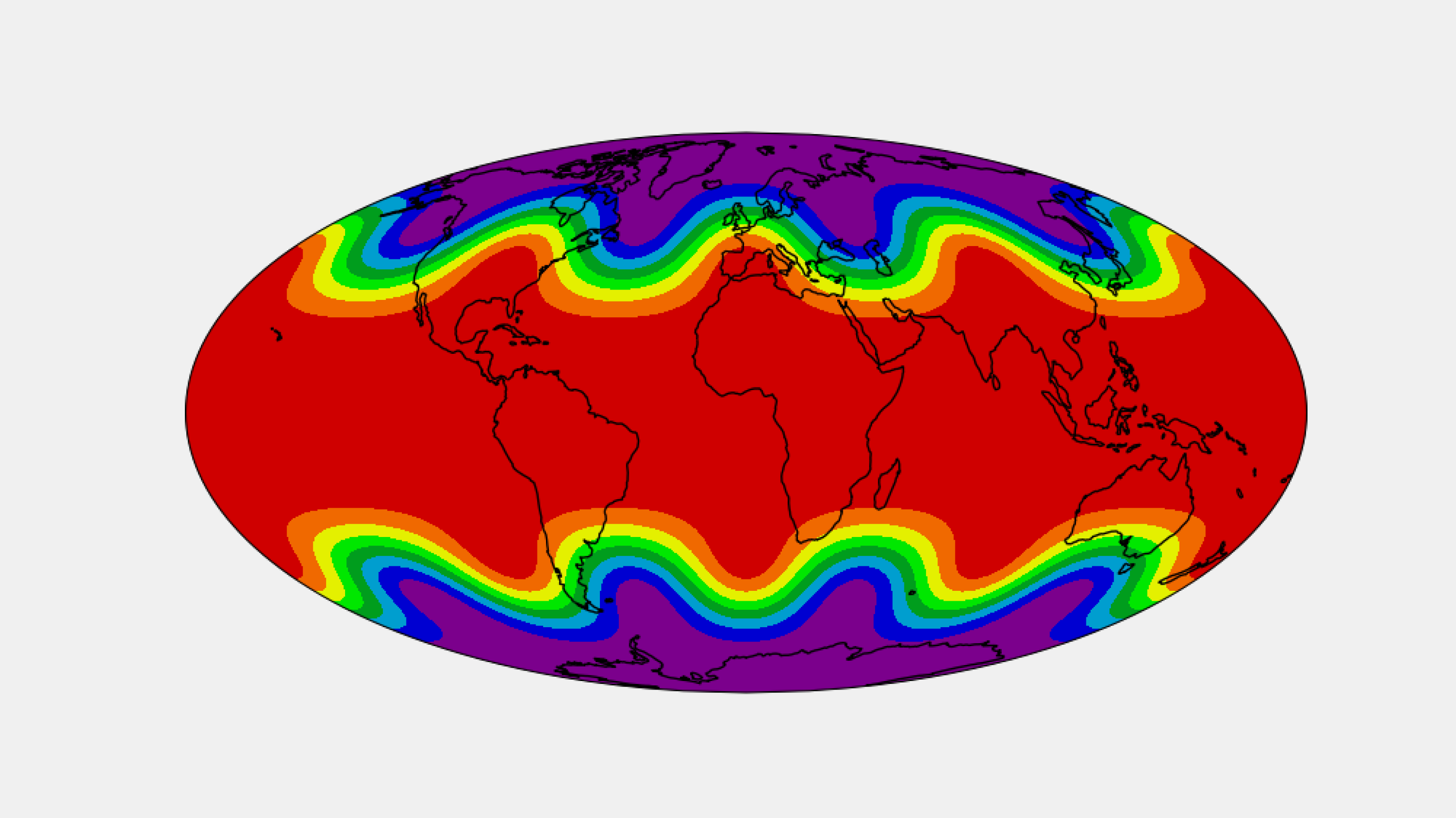
Изображение: Cartopy / SciTools
Сама Matplotlib является основой для других библиотек — например, Seaborn позволяет проще создавать графики и имеет больше возможностей для косметического улучшения их внешнего вида. Но Matplotlib — это базовая библиотека для визуализации данных, незаменимая в анализе данных.
При погружении в Matplotlib можно встретить упоминание двух модулей — Pyplot и Pylab. Важно понимать, какой из них использовать в работе и почему они появились. Разберёмся в терминологии.
Библиотека Matplotlib — это пакет для визуализации данных в Python. Pyplot — это модуль в пакете Matplotlib. Его вы часто будете видеть в коде как matplotlib.pyplot. Модуль помогает автоматически создавать оси, фигуры и другие компоненты, не задумываясь о том, как это происходит. Именно Pyplot используется в большинстве случаев.
Pylab — это ещё один модуль, который устанавливается вместе с пакетом Matplotlib. Он одновременно импортирует Pyplot и библиотеку NumPy для работы с массивами в интерактивном режиме или для доступа к функциям черчения при работе с данными.
Сейчас Pylab имеет только историческое значение — он облегчал переход с MATLAB на Matplotlib, так как позволял обходиться без операторов импорта (а именно так привыкли работать пользователи MATLAB). Вы можете встретиться с Pylab в примерах кода на разных сайтах, но на практике использовать модуль не придётся.
Matplotlib — универсальная библиотека, которая работает в Python на Windows, macOS и Linux. При работе с Google Colab или Jupyter Notebook устанавливать Python и Matplotlib не понадобится — язык программирования и библиотека уже доступны «из коробки». Но если вы решили писать код в другой IDE, например в Visual Studio Code, то сначала установите Python, а затем библиотеку Learn через терминал:
pip3 install matplotlib
Теперь можно переходить к импорту библиотеки:
import matplotlib.pyplot as plt
Сокращение plt для библиотеки — общепринятое. Вы встретите его в официальной документации, книгах и в ноутбуках других людей. Так что используйте его.
Для начала создадим две переменные — x и y, которые будут содержать координаты точек по осям х и у:
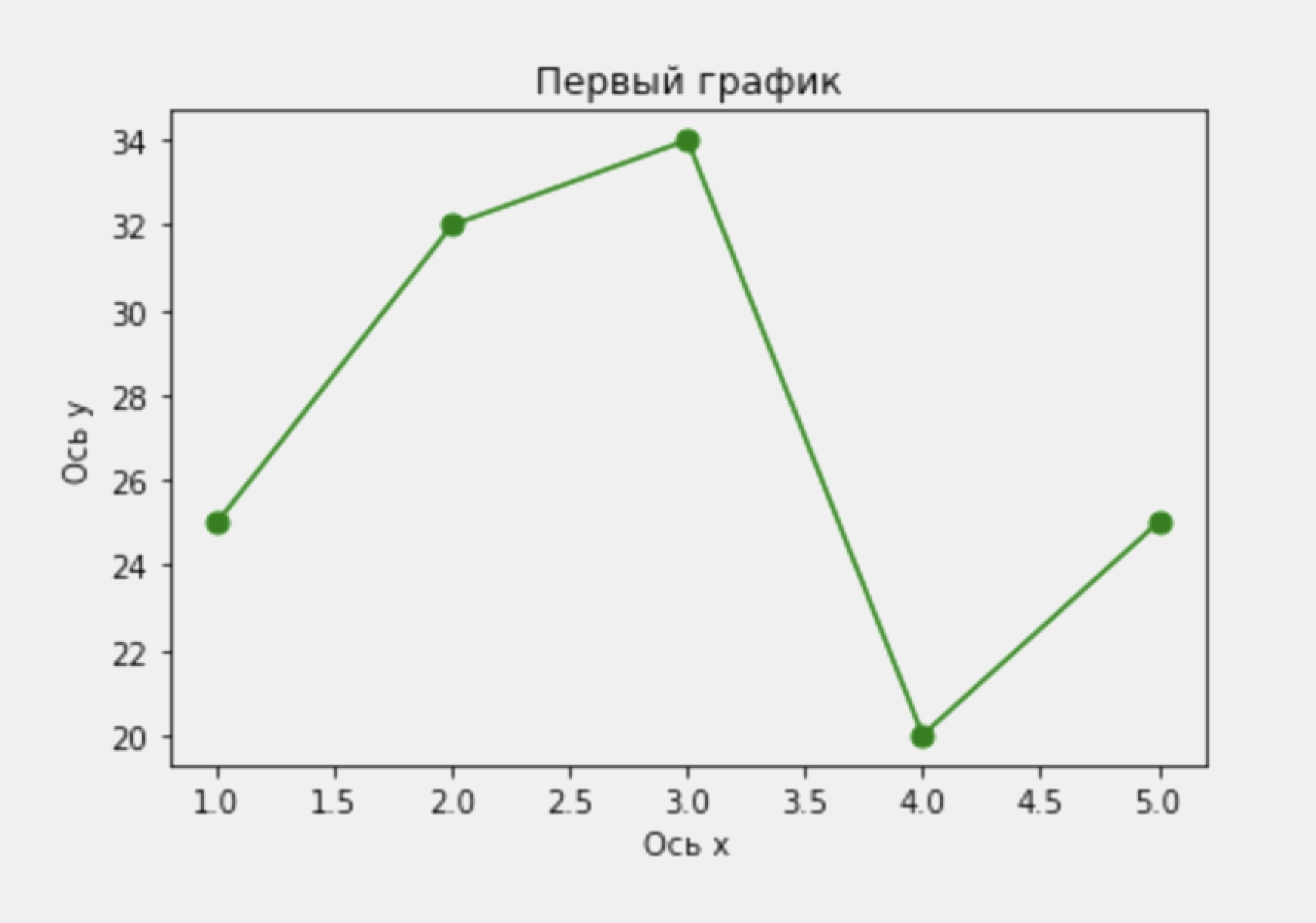
x = [1, 2, 3, 4, 5]
y = [25, 32, 34, 20, 25]
Теперь построим график, который соединит эти точки:
plt.plot(x, y)
plt.show()
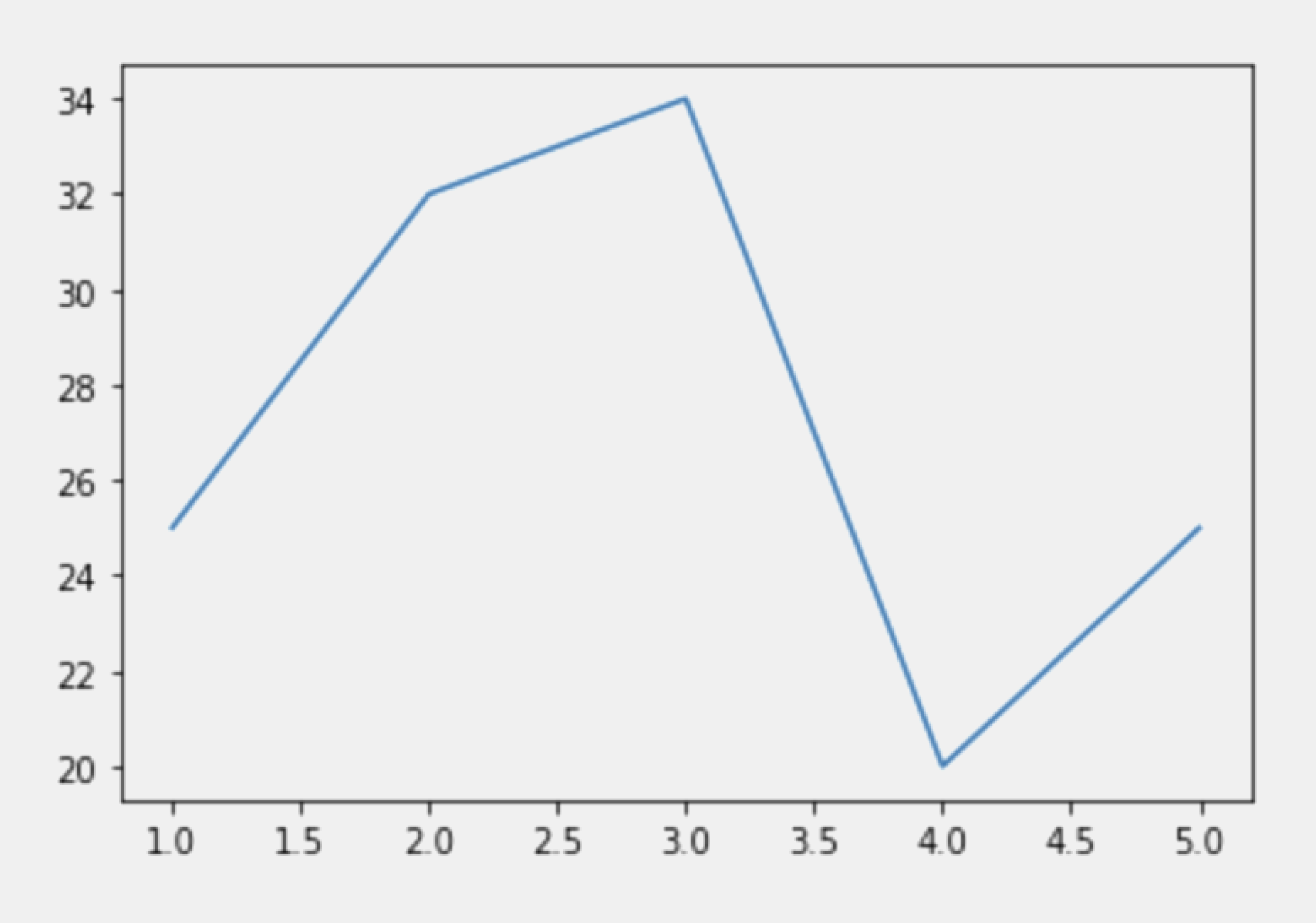
Мы получили обычный линейный график. Разберём каждую команду:
- plt.plot() — стандартная функция, которая строит график в соответствии со значениями, которые ей были переданы. Мы передали в неё координаты точек;
- plt.show() — функция, которая отвечает за вывод визуализированных данных на экран. Её можно и не указывать, но тогда, помимо красивой картинки, мы увидим разную техническую информацию.
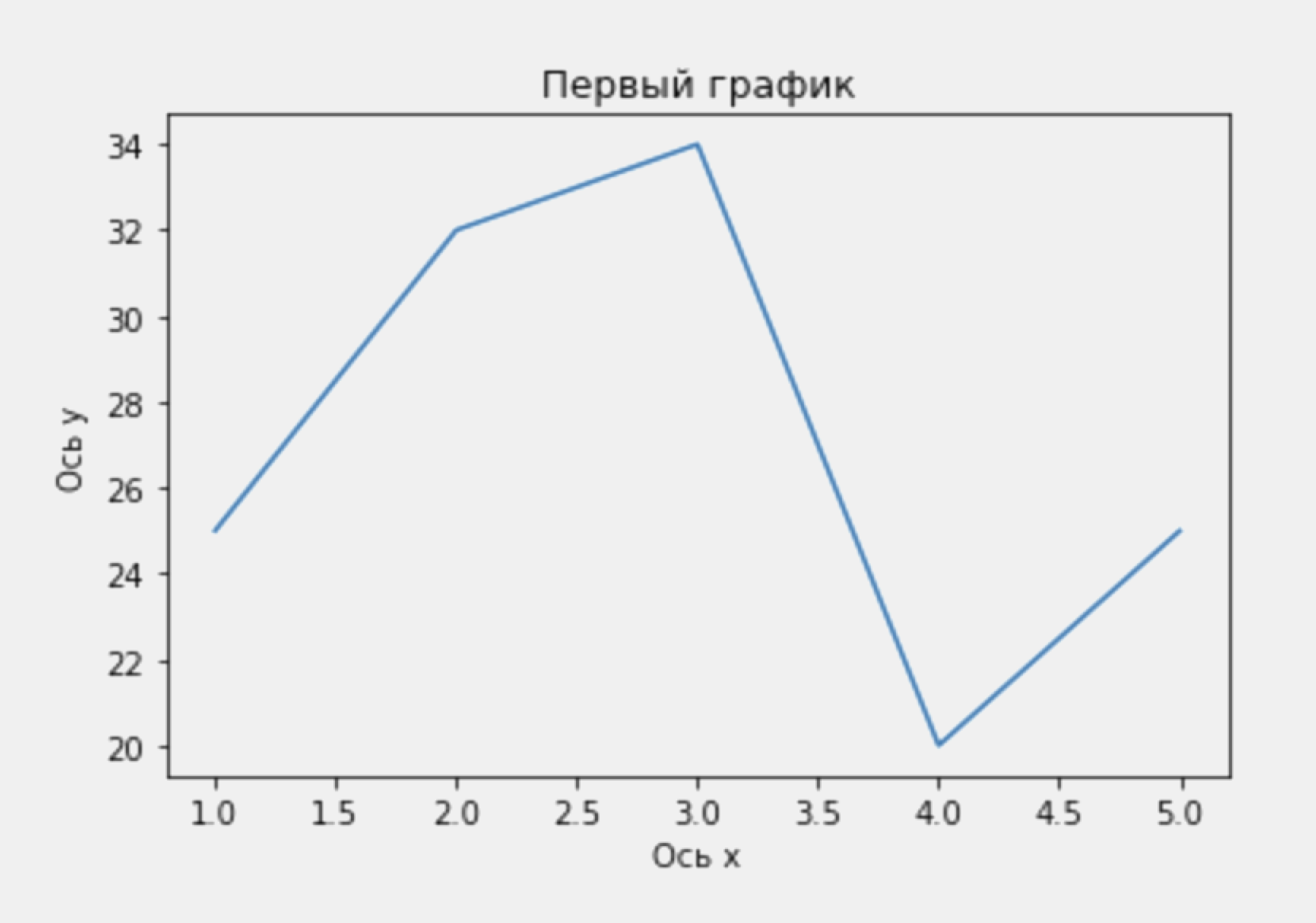
Дополним наш первый график заголовком и подписями осей:
plt.plot(x, y)
plt.xlabel('Ось х') #Подпись для оси х
plt.ylabel('Ось y') #Подпись для оси y
plt.title('Первый график') #Название
plt.show()
Смотрим на результат:
С помощью Matplotlib можно настроить отображение любого графика. Например, мы можем изменить цвет линии, а также выделить точки, координаты которых задаём в переменных:
plt.plot(x, y, color='green', marker='o', markersize=7)
Теперь точки хорошо видны, а цвет точек и линии изменился на зелёный:
Подробно про настройку параметров функции plt.plot() можно прочесть в официальной документации.
Диаграмма рассеяния используется для оценки взаимосвязи двух переменных, значения которых откладываются по разным осям. Для её построения используется функция plt.scatter(), аргументами которой выступают переменные с дискретными значениями:
x = [1, 2, 3, 4, 5, 6, 7, 8, 9, 10]
y = [25, 32, 34, 20, 25, 23, 21, 33, 19, 28]

plt.scatter(x, y)
plt.show()
Диаграмма рассеяния выглядит как множество отдельных точек:
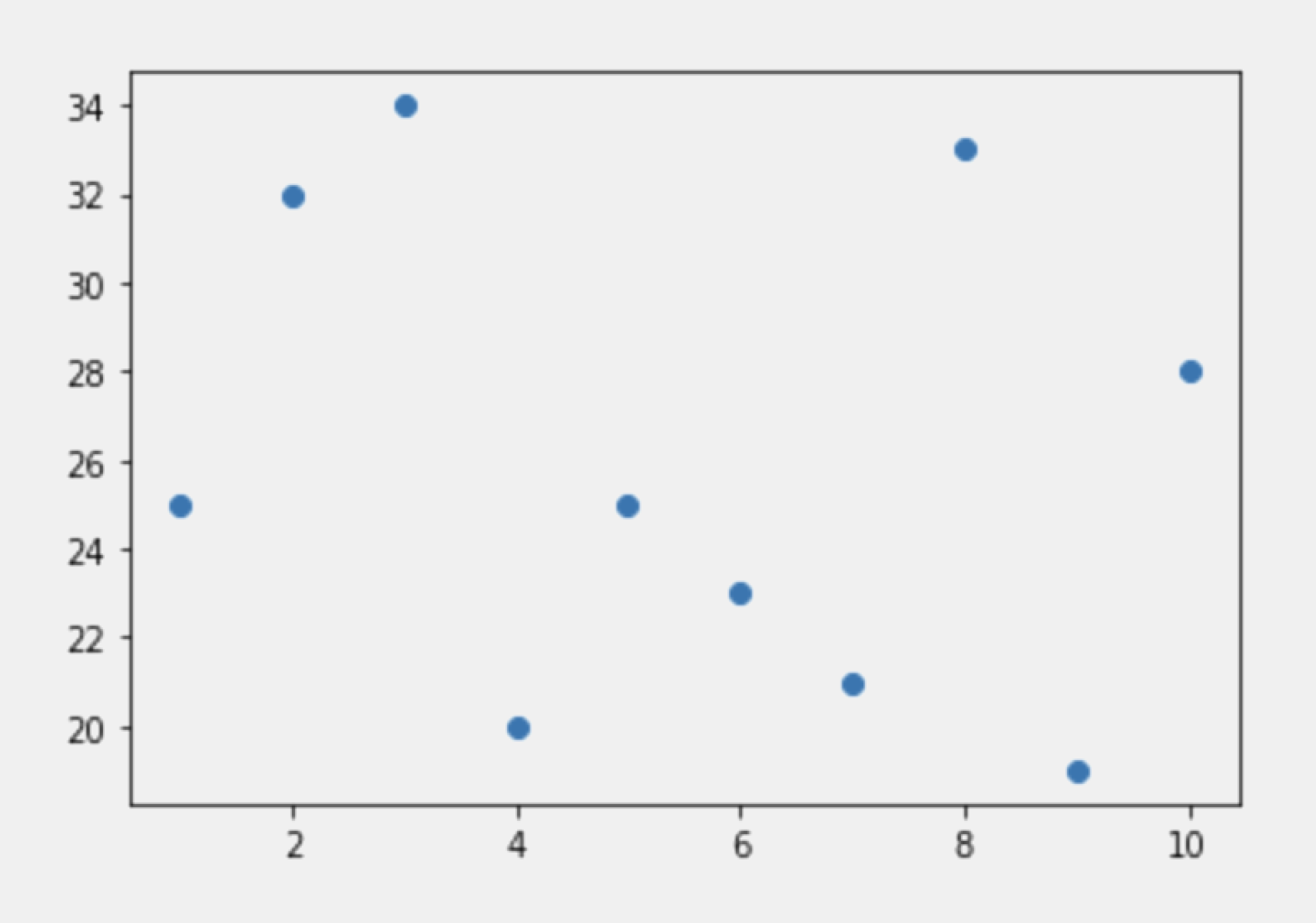
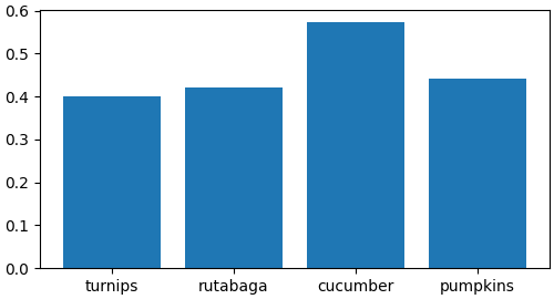
Такой тип визуализации позволяет удобно сравнивать значения отдельных переменных. В столбчатой диаграмме длина столбцов пропорциональна показателям, которые они отображают. Как правило, одна из осей соответствует одной категории, а вторая — её дискретному значению.
Например, столбчатая диаграмма позволяет наглядно показать величину прибыли по месяцам. Построим следующий график:
x = ['Январь', 'Февраль', 'Март', 'Апрель', 'Май']
y = [2, 4, 3, 1, 7]

plt.bar(x, y, label='Величина прибыли') #Параметр label позволяет задать название величины для легенды
plt.xlabel('Месяц года')
plt.ylabel('Прибыль, в млн руб.')
plt.title('Пример столбчатой диаграммы')
plt.legend()
plt.show()
Столбчатая диаграмма позволяет увидеть динамику изменения прибыли по месяцам:

Для некоторых задач полезно объединить несколько типов графиков, например столбчатую диаграмму и линейный график. Доработаем его, добавив к столбцам точки со значениями прибыли, и соединим их:
x = ['Январь', 'Февраль', 'Март', 'Апрель', 'Май']
y = [2, 4, 3, 1, 7]

plt.bar(x, y, label='Величина прибыли') #Параметр label позволяет задать название величины для легенды
plt.plot(x, y, color='green', marker='o', markersize=7)

plt.xlabel('Месяц года')
plt.ylabel('Прибыль, в млн руб.')
plt.title('Комбинирование графиков')
plt.legend()
plt.show()
Теперь на одном экране мы видим сразу оба типа:
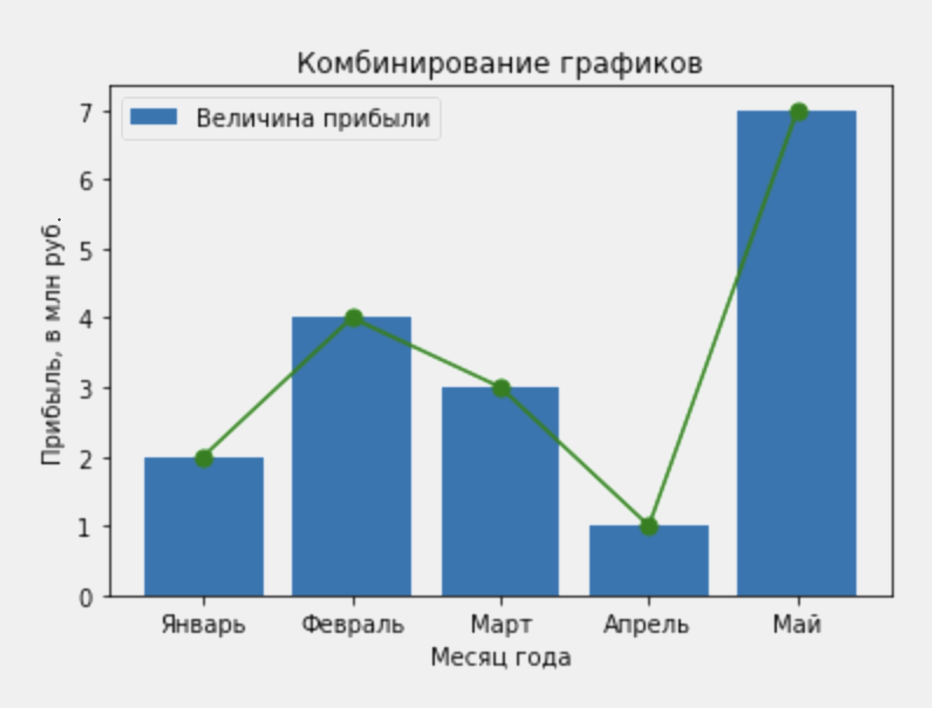
Всё получилось. Но сейчас линейный график видно плохо — он просто теряется на синем фоне столбцов. Увеличим прозрачность столбчатой диаграммы с помощью параметра alpha:
plt.bar(x, y, label='Величина прибыли', alpha=0.5)
Параметр alpha может принимать значения от 0 до 1, где 0 — полная прозрачность, а 1 — отсутствие прозрачности. Посмотрим на результат:
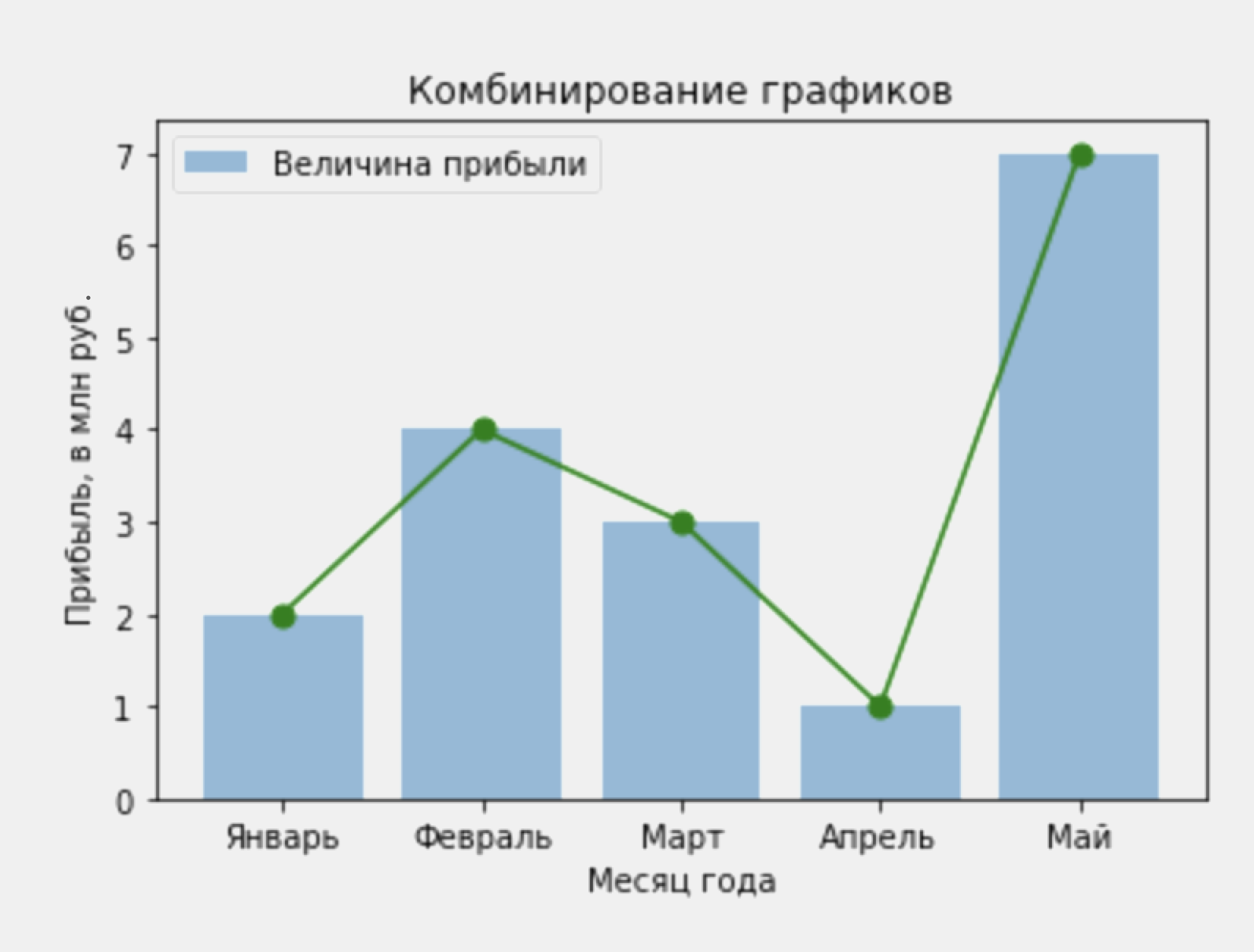
Теперь линейный график хорошо виден и мы можем оценивать динамику изменения прибыли.
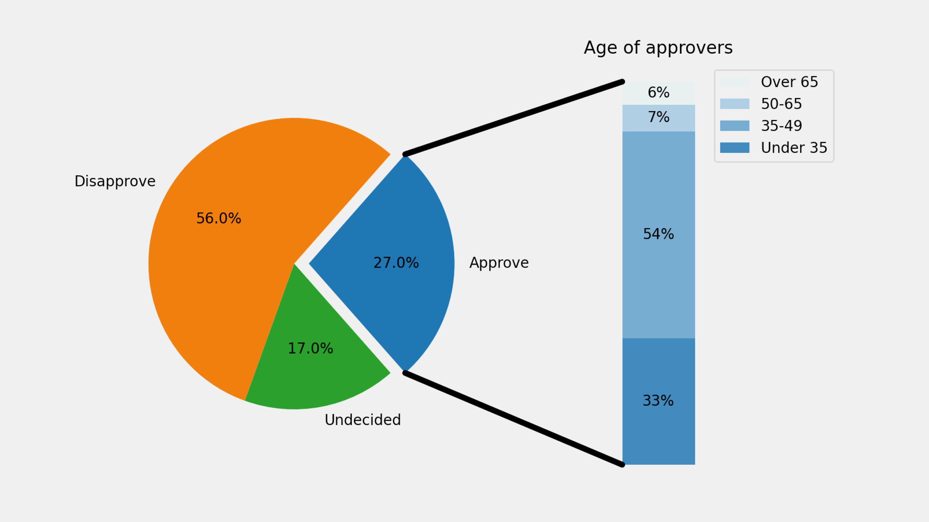
Круговую диаграмму используют для отображения состава групп. Например, мы можем наглядно показать, какие марки автомобилей преобладают на дорогах города:
vals = [24, 17, 53, 21, 35]
labels = ["Ford", "Toyota", "BMW", "Audi", "Jaguar"]

plt.pie(vals, labels=labels)
plt.title("Распределение марок автомобилей на дороге")
plt.show()
Результат:
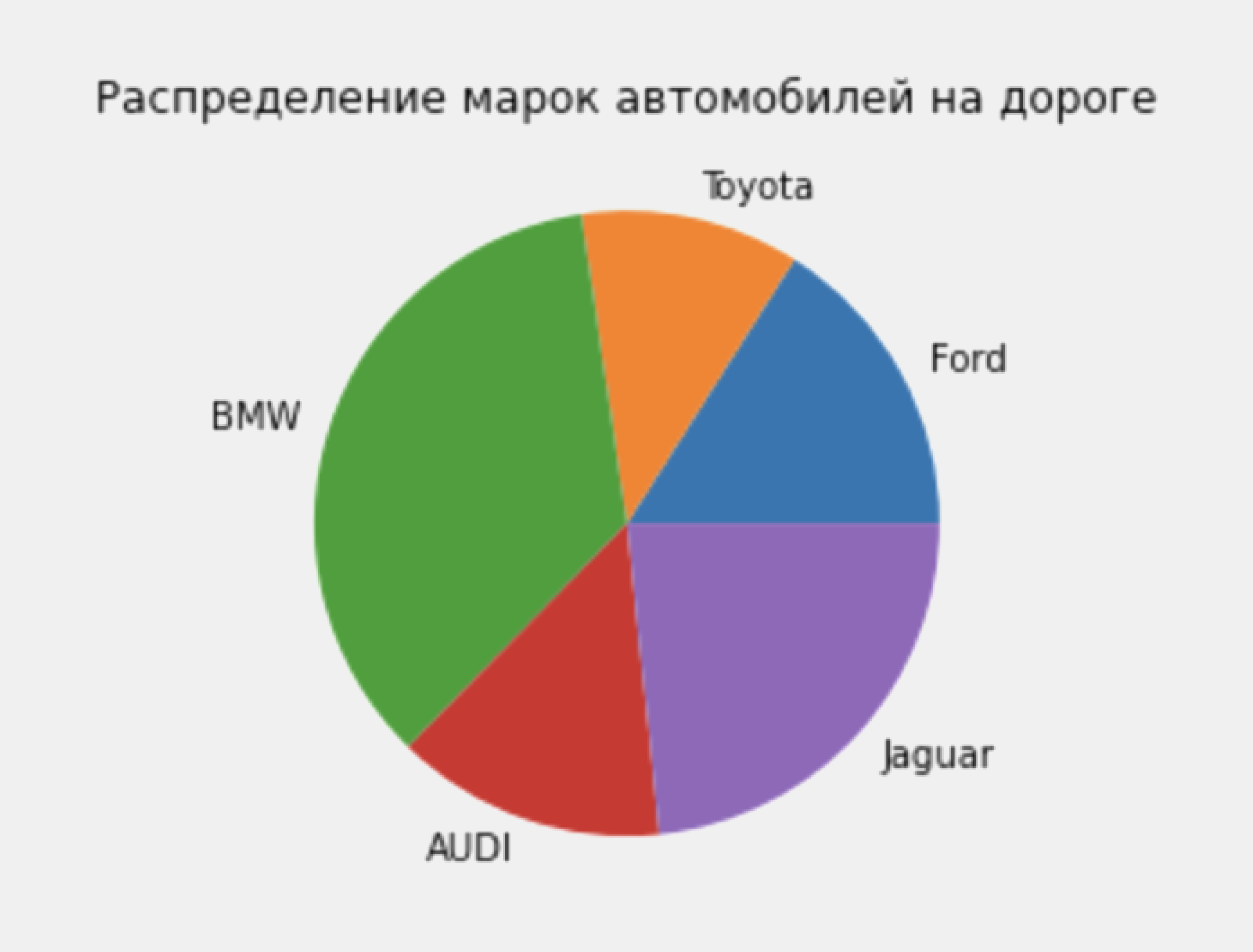
Так информация нагляднее, но непонятно, какая именно доля приходится на каждую марку автомобиля. Поэтому круговые диаграммы всегда лучше дополнять значениями в процентах. Отредактируем наш код, добавив к функции pie параметр autopct:
vals = [24, 17, 53, 21, 35]
labels = ["Ford", "Toyota", "BMW", "Audi", "Jaguar"]

plt.pie(vals, labels=labels, autopct='%1.1f%%')
plt.title("Распределение марок автомобилей на дороге")
plt.show()
В параметр мы передаём формат отображения числа. В нашем случае это будет целое число с одним знаком после запятой. Запустим код и посмотрим на результат:

Теперь сравнить категории проще, так как мы видим числовые значения.
Построим столбчатый график с накоплением. Он позволяет оценить динамику соотношения значений одной переменной. Попробуем показать, как соотносится количество устройств на Android и iOS в разные годы:
labels = ['2017', '2018', '2019', '2020', '2021']
android_users = [85, 85.1, 86, 86.2, 86]
ios_users = [14.5, 14.8, 13, 13.8, 14.0]

width = 0.35       #Задаём ширину столбцов
fig, ax = plt.subplots()

ax.bar(labels, android_users, width, label='Android')
ax.bar(labels, ios_users, width, bottom=android_users,
      label='iOS') #Указываем с помощью параметра bottom, что значения в столбце должны быть выше значений переменной android_users

ax.set_ylabel('Соотношение, в %')
ax.set_title('Распределение устройств на Android и iOS')
ax.legend(loc='lower left', title='Устройства') #Сдвигаем легенду в нижний левый угол, чтобы она не перекрывала часть графика

plt.show()
Смотрим на результат:
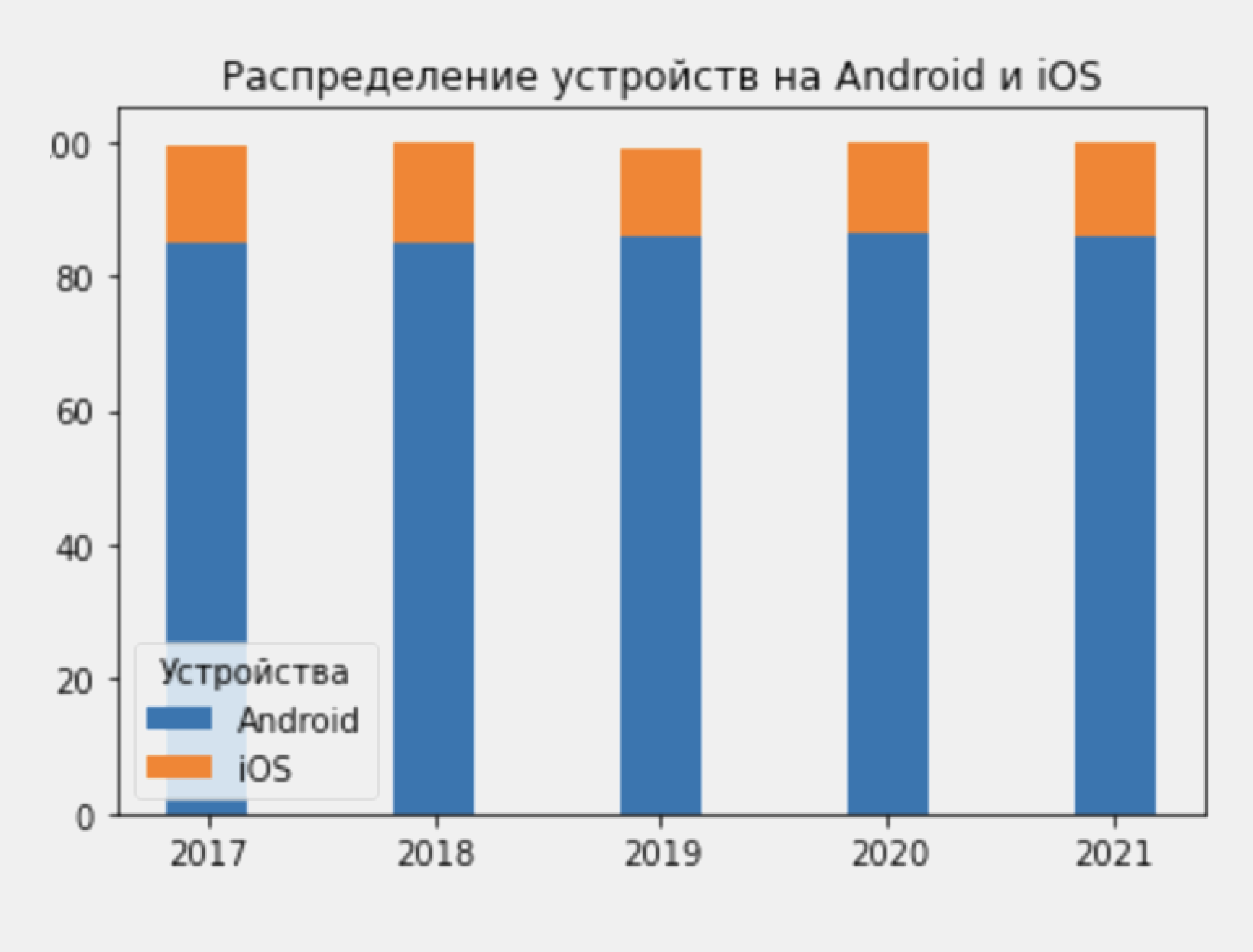
График позволяет увидеть, что соотношение устройств, работающих на Android и iOS, постепенно меняется — устройств на Android становится больше.
Matplotlib — мощная библиотека для визуализации данных в Python. В этой статье мы познакомились только с самыми основами. Ещё много полезной информации можно найти в официальной документации.
Но если вы решили действительно углубиться в возможности библиотеки и визуализацию данных, то здесь помогут книги:
- Mastering matplotlib Дункана Макгреггора;
- Hands-on Matplotlib: Learn Plotting and Visualizations with Python 3 Ашвина Паянкара;
- Matplotlib 3.0 Cookbook: Over 150 recipes to create highly detailed interactive visualizations using Python Рао Полади.

Научитесь: Профессия Python-разработчик
Узнать больше
Matplotlib – Введение
Matplotlib – один из самых популярных пакетов Python, используемых для визуализации данных. Это кроссплатформенная библиотека для создания 2D графиков из данных в массивах. Matplotlib написан на Python и использует NumPy, числовое математическое расширение Python. Он предоставляет объектно-ориентированный API, который помогает встраивать графики в приложения, используя наборы инструментов Python GUI, такие как PyQt, WxPythonotTkinter. Он также может использоваться в оболочках Python и IPython, ноутбуках Jupyter и серверах веб-приложений.
Matplotlib имеет процедурный интерфейс под названием Pylab, который похож на MATLAB, проприетарный язык программирования, разработанный MathWorks. Matplotlib вместе с NumPy можно рассматривать как эквивалент MATLAB с открытым исходным кодом.
Matplotlib был первоначально написан Джоном Д. Хантером в 2003 году. Текущая стабильная версия 2.2.0 выпущена в январе 2018 года.
Matplotlib – Настройка среды
Matplotlib и его пакеты зависимостей доступны в виде пакетов wheel в стандартных репозиториях пакетов Python и могут быть установлены в системах Windows, Linux, а также MacOS с помощью диспетчера пакетов pip.
pip3 install matplotlib
Incase версии Python 2.7 или 3.4 установлены не для всех пользователей, необходимо установить распространяемые пакеты Microsoft Visual C ++ 2008 (64-разрядная или 32-разрядная версия для Python 2.7) или Microsoft Visual C ++ 2010 (64-разрядная или 32-разрядная версия для Python 3.4).
Если вы используете Python 2.7 на Mac, выполните следующую команду –
xcode-select –install
После выполнения вышеприведенной команды подпроцесс 32 – зависимость может быть скомпилирован.
В чрезвычайно старых версиях Linux и Python 2.7 может потребоваться установить основную версию подпроцесса32.
Matplotlib требует большого количества зависимостей –
- Python (> = 2,7 или> = 3,4)
- NumPy
- Setuptools
- dateutil
- Pyparsing
- Libpng
- pytz
- FreeType
- велосипедист
- шесть
При желании вы также можете установить несколько пакетов, чтобы активировать лучшие инструменты интерфейса пользователя.
- тк
- PyQt4
- PyQt5
- PyGTK
- WxPython
- pycairo
- Торнадо
Для лучшей поддержки формата вывода анимации и форматов файлов изображений, LaTeX и т. Д. Вы можете установить следующее:
- _mpeg / avconv
- ImageMagick
- Подушка (> = 2.0)
- LaTeX и GhostScript (для рендеринга текста с помощью LaTeX).
- LaTeX и GhostScript (для рендеринга текста с помощью LaTeX).
Матплотлиб – Анаконда дистрибуция
Anaconda – это бесплатный и открытый исходный код языков программирования Python и R для крупномасштабной обработки данных, прогнозной аналитики и научных вычислений. Распределение делает управление пакетами и развертывание простым и легким. Matplotlib и множество других полезных (data) научных инструментов являются частью дистрибутива. Версии пакетов управляются системой управления пакетами Conda. Преимущество Anaconda заключается в том, что у вас есть доступ к более чем 720 пакетам, которые можно легко установить с помощью Andaonda Conda, менеджера пакетов, зависимостей и среды.
Дистрибутив Anaconda доступен для установки по адресу https://www.anaconda.com/download/. Для установки в Windows доступны 32 и 64-битные бинарные файлы –
https://repo.continuum.io/archive/Anaconda3-5.1.0-Windows-x86.exe
https://repo.continuum.io/archive/Anaconda3-5.1.0-Windows-x86_64.exe
Установка является довольно простым процессом на основе мастера. Вы можете выбрать между добавлением Anaconda в переменную PATH и регистрацией Anaconda в качестве Python по умолчанию.
Для установки в Linux загрузите установщики для 32-разрядных и 64-разрядных установщиков со страницы загрузок –
https://repo.continuum.io/archive/Anaconda3-5.1.0-Linux-x86.sh
https://repo.continuum.io/archive/Anaconda3-5.1.0-Linux-x86_64.sh
Теперь запустите следующую команду из терминала Linux –
$ bash Anaconda3-5.0.1-Linux-x86_64.sh
Canopy и ActiveState – наиболее востребованные решения для Windows, macOS и распространенных платформ Linux. Пользователи Windows могут найти опцию в WinPython.
Matplotlib – ноутбук Юпитер
Jupyter – это аббревиатура, означающая Julia, Python и R. Эти языки программирования были первыми целевыми языками приложения Jupyter, но в настоящее время технология ноутбука также поддерживает многие другие языки.
В 2001 году Фернандо Перес начал разработку Ipython. IPython – это командная оболочка для интерактивных вычислений на нескольких языках программирования, изначально разработанная для Python.
Рассмотрим следующие возможности, предоставляемые IPython –
-
Интерактивные оболочки (на основе терминала и Qt).
-
Записная книжка на основе браузера с поддержкой кода, текста, математических выражений, встроенных графиков и других средств массовой информации.
-
Поддержка интерактивной визуализации данных и использование инструментария GUI.
-
Гибкие, встраиваемые интерпретаторы для загрузки в собственные проекты.
Интерактивные оболочки (на основе терминала и Qt).
Записная книжка на основе браузера с поддержкой кода, текста, математических выражений, встроенных графиков и других средств массовой информации.
Поддержка интерактивной визуализации данных и использование инструментария GUI.
Гибкие, встраиваемые интерпретаторы для загрузки в собственные проекты.
В 2014 году Фернандо Перес анонсировал дополнительный проект от IPython под названием Project Jupyter. IPython будет продолжать существовать как оболочка Python и ядро для Jupyter, в то время как блокнот и другие не зависящие от языка части IPython будут перемещаться под именем Jupyter. Jupyter добавил поддержку для Julia, R, Haskell и Ruby.
Чтобы запустить ноутбук Jupyter, откройте навигатор Anaconda (графический интерфейс пользователя на рабочем столе, включенный в Anaconda, который позволяет запускать приложения и легко управлять пакетами, средами и каналами Conda без необходимости использования команд командной строки).
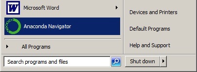
Навигатор отображает установленные компоненты в дистрибутиве.
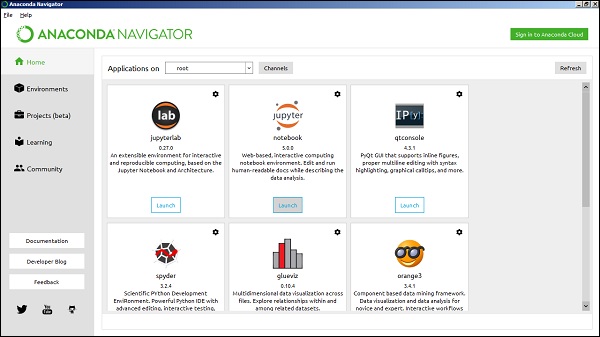
Запустите Jupyter Notebook из навигатора –
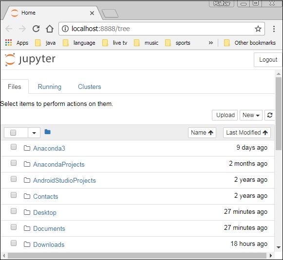
Вы увидите открытие приложения в веб-браузере по следующему адресу – http: // localhost: 8888.

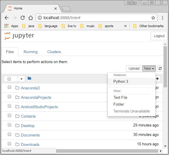
Вы, вероятно, хотите начать с создания нового ноутбука. Вы можете легко сделать это, нажав на кнопку «Создать» на вкладке «Файлы». Вы видите, что у вас есть возможность сделать обычный текстовый файл, папку и терминал. Наконец, вы также увидите возможность сделать ноутбук на Python 3.
Matplotlib – Pyplot API
Новый блокнот без названия с расширением .ipynb (расшифровывается как блокнот IPython) отображается на новой вкладке браузера.

matplotlib.pyplot – это набор функций командного стиля, которые делают Matplotlib похожим на MATLAB. Каждая функция Pyplot вносит некоторые изменения в фигуру. Например, функция создает фигуру, область построения на рисунке, строит некоторые линии в области построения, украшает график метками и т. Д.
Типы участков
| Sr.No | Описание функции |
|---|---|
| 1 |
Бар Сделайте барный сюжет. |
| 2 |
Барх Сделайте горизонтальный линейный график. |
| 3 |
Boxplot Сделать коробку и усы сюжет. |
| 4 |
тс Постройте гистограмму. |
| 5 |
hist2d Создайте 2D гистограмму. |
| 6 |
пирог Постройте круговую диаграмму. |
| 7 |
участок Нанесите линии и / или маркеры на оси. |
| 8 |
полярный Сделай полярный сюжет .. |
| 9 |
рассеивать Составьте точечный график x против y. |
| 10 |
Stackplot Рисует сложенную область участка. |
| 11 |
ножка Создайте сюжетный ствол. |
| 12 |
шаг Сделайте пошаговый сюжет. |
| 13 |
Колчан Постройте двумерное поле стрелок. |
Бар
Сделайте барный сюжет.
Барх
Сделайте горизонтальный линейный график.
Boxplot
Сделать коробку и усы сюжет.
тс
Постройте гистограмму.
hist2d
Создайте 2D гистограмму.
пирог
Постройте круговую диаграмму.
участок
Нанесите линии и / или маркеры на оси.
полярный
Сделай полярный сюжет ..
рассеивать
Составьте точечный график x против y.
Stackplot
Рисует сложенную область участка.
ножка
Создайте сюжетный ствол.
шаг
Сделайте пошаговый сюжет.
Колчан
Постройте двумерное поле стрелок.
Функции изображения
| Sr.No | Описание функции |
|---|---|
| 1 |
Imread Прочитать изображение из файла в массив. |
| 2 |
Imsave Сохраните массив как в файле изображения. |
| 3 |
Imshow Покажите изображение на осях. |
Imread
Прочитать изображение из файла в массив.
Imsave
Сохраните массив как в файле изображения.
Imshow
Покажите изображение на осях.
Функции оси
| Sr.No | Описание функции |
|---|---|
| 1 |
Топоры Добавьте оси к фигуре. |
| 2 |
Текст Добавьте текст к осям. |
| 3 |
заглавие Установить заголовок текущих осей. |
| 4 |
Xlabel Установите метку оси x текущей оси. |
| 5 |
Xlim Получить или установить пределы х текущих осей. |
| 6 |
Xscale , |
| 7 |
Xticks Получить или установить x-пределы текущего местоположения галочек и меток. |
| 8 |
Ylabel Установите метку оси Y текущей оси. |
| 9 |
Ylim Получить или установить Y-пределы текущих осей. |
| 10 |
Yscale Установите масштаб оси Y. |
| 11 |
Yticks Получите или установите y-пределы текущего местоположения галочки и меток. |
Топоры
Добавьте оси к фигуре.
Текст
Добавьте текст к осям.
заглавие
Установить заголовок текущих осей.
Xlabel
Установите метку оси x текущей оси.
Xlim
Получить или установить пределы х текущих осей.
Xscale
,
Xticks
Получить или установить x-пределы текущего местоположения галочек и меток.
Ylabel
Установите метку оси Y текущей оси.
Ylim
Получить или установить Y-пределы текущих осей.
Yscale
Установите масштаб оси Y.
Yticks
Получите или установите y-пределы текущего местоположения галочки и меток.
Функции рисунка
| Sr.No | Описание функции |
|---|---|
| 1 |
Figtext Добавьте текст к рисунку. |
| 2 |
фигура Создает новую фигуру. |
| 3 |
Шоу Покажите фигуру. |
| 4 |
Savefig Сохранить текущий рисунок. |
| 5 |
близко Закройте окно фигуры. |
Figtext
Добавьте текст к рисунку.
фигура
Создает новую фигуру.
Шоу
Покажите фигуру.
Savefig
Сохранить текущий рисунок.
близко
Закройте окно фигуры.
Matplotlib – простой сюжет
В этой главе мы узнаем, как создать простой график с помощью Matplotlib.
Теперь мы покажем простой линейный график угла в радианах относительно его значения синуса в Matplotlib. Начнем с того, что модуль Pyplot из пакета Matplotlib импортируется с псевдонимом plt по договоренности.
import matplotlib.pyplot as plt
Далее нам нужен массив чисел для построения. Различные функции массива определены в библиотеке NumPy, которая импортируется с псевдонимом np.
import numpy as np
Теперь мы получаем ndarray объект углов между 0 и 2π, используя функцию arange () из библиотеки NumPy.
x = np.arange(0, math.pi*2, 0.05)
Объект ndarray служит значениями на оси x графика. Соответствующие значения синусов углов в x, которые будут отображены на оси y, получаются с помощью следующего оператора –
y = np.sin(x)
Значения из двух массивов построены с использованием функции plot ().
plt.plot(x,y)
Вы можете установить название графика и метки для осей x и y.
You can set the plot title, and labels for x and y axes.
plt.xlabel("angle")
plt.ylabel("sine")
plt.title('sine wave')
Окно просмотра графика вызывается функцией show () –
plt.show()
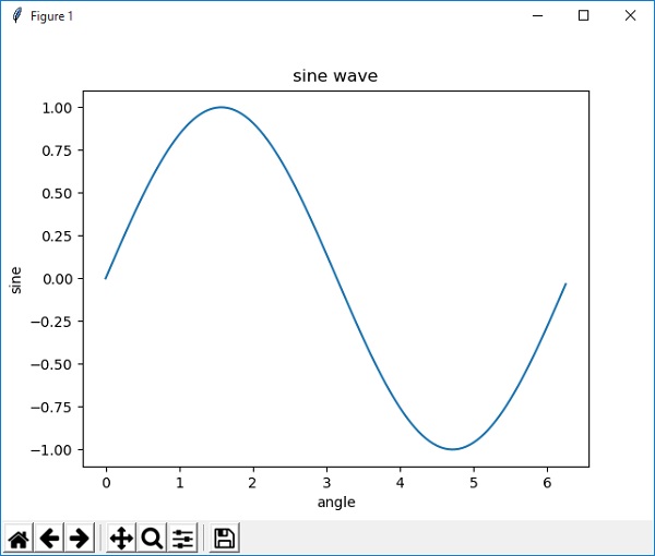
Полная программа выглядит следующим образом –
from matplotlib import pyplot as plt
import numpy as np
import math #needed for definition of pi
x = np.arange(0, math.pi*2, 0.05)
y = np.sin(x)
plt.plot(x,y)
plt.xlabel("angle")
plt.ylabel("sine")
plt.title('sine wave')
plt.show()
Когда вышеуказанная строка кода выполняется, отображается следующий график –
Теперь используйте ноутбук Jupyter с Matplotlib.
Запустите блокнот Jupyter из навигатора Anaconda или из командной строки, как описано ранее. В ячейке ввода введите операторы импорта для Pyplot и NumPy –
from matplotlib import pyplot as plt
import numpy as np
Чтобы отобразить результаты печати внутри самой записной книжки (а не в отдельной программе просмотра), введите следующее волшебное утверждение –
%matplotlib inline
Получите x как ndarray объект, содержащий углы в радианах от 0 до 2π, а y как синусоидальную величину каждого угла –
import math
x = np.arange(0, math.pi*2, 0.05)
y = np.sin(x)
Установите метки для осей X и Y, а также название графика –
plt.xlabel("angle")
plt.ylabel("sine")
plt.title('sine wave')
Наконец, выполните функцию plot () для генерации синусоидального изображения в записной книжке (нет необходимости запускать функцию show ()) –
plt.plot(x,y)
После выполнения последней строки кода отображается следующий вывод:

Matplotlib – модуль PyLab
PyLab – это процедурный интерфейс к библиотеке объектно-ориентированных графиков Matplotlib. Matplotlib – это целый пакет; matplotlib.pyplot – это модуль в Matplotlib; PyLab – это модуль, который устанавливается вместе с Matplotlib.
PyLab – это удобный модуль, который массово импортирует matplotlib.pyplot (для построения графиков) и NumPy (для математики и работы с массивами) в одном пространстве имен. Хотя во многих примерах используется PyLab, он больше не рекомендуется.
Основы печати
Построение кривых выполняется с помощью команды plot. Требуется пара массивов одинаковой длины (или последовательности) –
from numpy import *
from pylab import *
x = linspace(-3, 3, 30)
y = x**2
plot(x, y)
show()
Выше строка кода генерирует следующий вывод –

Чтобы отобразить символы, а не линии, укажите дополнительный строковый аргумент.
| символы | -, -, -.,,. ,,, о, ^, v, <,>, с, +, х, D, д, 1, 2, 3, 4, ч, Н, р, | , _ |
| цвета | b, g, r, c, m, y, k, w |
Теперь рассмотрим выполнение следующего кода –
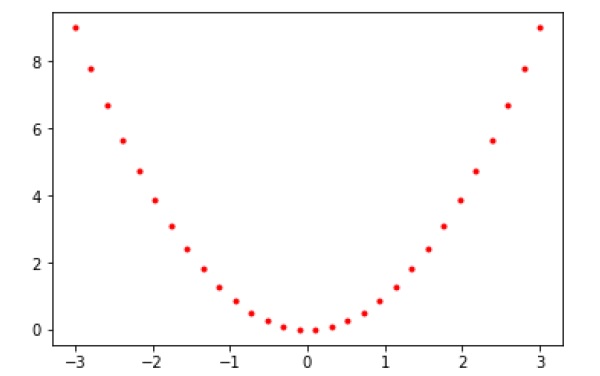
from pylab import *
x = linspace(-3, 3, 30)
y = x**2
plot(x, y, 'r.')
show()
Он отображает красные точки, как показано ниже –
Участки могут быть наложены. Просто используйте несколько команд заговора. Используйте clf (), чтобы очистить график.
from pylab import *
plot(x, sin(x))
plot(x, cos(x), 'r-')
plot(x, -sin(x), 'g--')
show()
Выше строка кода генерирует следующий вывод –

Matplotlib – объектно-ориентированный интерфейс
Несмотря на то, что с помощью модуля matplotlib.pyplot легко быстро создавать графики, рекомендуется использовать объектно-ориентированный подход, поскольку он обеспечивает больший контроль и настройку ваших графиков. Большинство функций также доступны в классе matplotlib.axes.Axes .
Основная идея использования более формального объектно-ориентированного метода состоит в том, чтобы создавать объекты фигур, а затем просто вызывать методы или атрибуты этого объекта. Этот подход помогает лучше справляться с холстом, на котором есть несколько графиков.
В объектно-ориентированном интерфейсе Pyplot используется только для нескольких функций, таких как создание фигур, а пользователь явно создает и отслеживает объекты фигур и осей. На этом уровне пользователь использует Pyplot для создания фигур, и с помощью этих фигур можно создавать один или несколько объектов осей. Эти объекты осей затем используются для большинства графических действий.
Для начала мы создаем экземпляр фигуры, который предоставляет пустой холст.
fig = plt.figure()
Теперь добавьте оси к фигуре. Метод add_axes () требует объекта списка из 4 элементов, соответствующих левому, нижнему, ширине и высоте фигуры. Каждое число должно быть от 0 до 1 –
ax=fig.add_axes([0,0,1,1])
Установить метки для осей X и Y, а также заголовок –
ax.set_title("sine wave")
ax.set_xlabel('angle')
ax.set_ylabel('sine')
Вызвать метод plot () объекта оси.
ax.plot(x,y)
Если вы используете ноутбук Jupyter, должна быть выпущена встроенная директива% matplotlib; функция otherwistshow () модуля pyplot отображает график.
Попробуйте выполнить следующий код –
from matplotlib import pyplot as plt
import numpy as np
import math
x = np.arange(0, math.pi*2, 0.05)
y = np.sin(x)
fig = plt.figure()
ax = fig.add_axes([0,0,1,1])
ax.plot(x,y)
ax.set_title("sine wave")
ax.set_xlabel('angle')
ax.set_ylabel('sine')
plt.show()
Выход
Выше строка кода генерирует следующий вывод –

Тот же код при запуске в блокноте Jupyter показывает вывод, как показано ниже –

Matplotlib – класс рисунков
Модуль matplotlib.figure содержит класс Figure. Это контейнер верхнего уровня для всех элементов графика. Создание объекта Figure осуществляется путем вызова функции figure () из модуля pyplot –
fig = plt.figure()
В следующей таблице приведены дополнительные параметры –
| Figsize | (ширина, высота) кортеж в дюймах |
| точек на дюйм | Точек на дюймы |
| Facecolor | Рисунок патча лицевого цвета |
| Edgecolor | Рисунок края пятна цвета |
| Ширина линии | Ширина линии края |
Matplotlib – класс топоров
Объект оси – это область изображения с пространством данных. Данная фигура может содержать много осей, но данный объект осей может быть только на одной фигуре. Оси содержат два (или три в случае 3D) объекта Оси. Класс Axes и его функции-члены являются основной точкой входа в работу с интерфейсом OO.
Объект Axes добавляется к рисунку путем вызова метода add_axes (). Он возвращает объект осей и добавляет оси в позиции rect [left, bottom, width, height], где все величины выражены в долях ширины и высоты фигуры.
параметр
Ниже приведен параметр для класса Axes –
-
rect – последовательность из четырех величин [влево, низ, ширина, высота].
rect – последовательность из четырех величин [влево, низ, ширина, высота].
ax=fig.add_axes([0,0,1,1])
Следующие функции-члены класса осей добавляют разные элементы в plot –
легенда
Метод legend () класса осей добавляет легенду на график. Требуется три параметра –
ax.legend(handles, labels, loc)
Где метки представляют собой последовательность строк и обрабатывают последовательность экземпляров Line2D или Patch. loc может быть строкой или целым числом, указывающим местоположение легенды.
| Строка местоположения | Код местоположения |
|---|---|
| Лучший | 0 |
| верхний правый | 1 |
| верхний левый | 2 |
| нижний левый | 3 |
| Нижний правый | 4 |
| Правильно | 5 |
| Центр слева | 6 |
| Правый центр | 7 |
| нижний центр | 8 |
| верхний центр | 9 |
| Центр | 10 |
axes.plot ()
Это основной метод класса осей, который отображает значения одного массива относительно другого в виде линий или маркеров. Метод plot () может иметь необязательный аргумент строки формата для указания цвета, стиля и размера линии и маркера.
Цветовые коды
| символ | цвет |
|---|---|
| «Б» | синий |
| ‘г’ | зеленый |
| ‘р’ | красный |
| «Б» | синий |
| «С» | Cyan |
| «М» | фуксин |
| «У» | желтый |
| «К» | черный |
| «Б» | синий |
| «Ш» | белый |
Коды маркеров
| символ | Описание |
|---|---|
| ” | Маркер точки |
| «О» | Маркер круга |
| ‘Икс’ | Маркер X |
| ‘D’ | Алмазный маркер |
| ‘ЧАС’ | Маркер шестиугольника |
| ‘S’ | Квадратный маркер |
| ‘+’ | Плюс маркер |
Стили линий
| символ | Описание |
|---|---|
| ‘-‘ | Сплошная линия |
| ‘-‘ | Пунктир |
| ‘-‘. | Пунктирная линия |
| ‘:’ | Пунктирная линия |
| ‘ЧАС’ | Маркер шестиугольника |
В следующем примере показаны расходы на рекламу и продажи телевизоров и смартфонов в виде линейных графиков. Линия, представляющая телевизор, представляет собой сплошную линию с желтым цветом и квадратными маркерами, а линия смартфона – пунктирная линия с зеленым цветом и круговым маркером.
import matplotlib.pyplot as plt
y = [1, 4, 9, 16, 25,36,49, 64]
x1 = [1, 16, 30, 42,55, 68, 77,88]
x2 = [1,6,12,18,28, 40, 52, 65]
fig = plt.figure()
ax = fig.add_axes([0,0,1,1])
l1 = ax.plot(x1,y,'ys-') # solid line with yellow colour and square marker
l2 = ax.plot(x2,y,'go--') # dash line with green colour and circle marker
ax.legend(labels = ('tv', 'Smartphone'), loc = 'lower right') # legend placed at lower right
ax.set_title("Advertisement effect on sales")
ax.set_xlabel('medium')
ax.set_ylabel('sales')
plt.show()
Когда приведенная выше строка кода выполняется, она создает следующий график –

Матплотлиб – Мультиплоты
В этой главе мы научимся создавать несколько сюжетов на одном холсте.
Функция subplot () возвращает объект оси в заданной позиции сетки. Сигнатура Call этой функции –
plt.subplot(subplot(nrows, ncols, index)
На текущем рисунке функция создает и возвращает объект Axes с указателем позиции сетки nrows по ncolsaxes. Индексы изменяются от 1 до nrows * ncols с приращением в главном порядке строк. Если значение параметраrow, ncols и index меньше 10, индексы также могут быть заданы как одно объединенное, threedigitnumber.
Например, как вспомогательный участок (2, 3, 3), так и вспомогательный участок (233) создают оси в верхнем правом углу текущей фигуры, занимая половину высоты фигуры и треть ширины фигуры.
Создание подзаголовка приведет к удалению любого ранее существующего подплота, который перекрывается с ним за пределами общей границы.
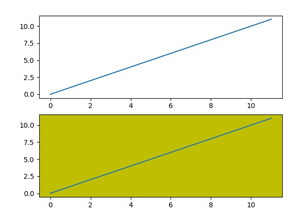
import matplotlib.pyplot as plt
# plot a line, implicitly creating a subplot(111)
plt.plot([1,2,3])
# now create a subplot which represents the top plot of a grid with 2 rows and 1 column.
#Since this subplot will overlap the first, the plot (and its axes) previously
created, will be removed
plt.subplot(211)
plt.plot(range(12))
plt.subplot(212, facecolor='y') # creates 2nd subplot with yellow background
plt.plot(range(12))
Выше строка кода генерирует следующий вывод –
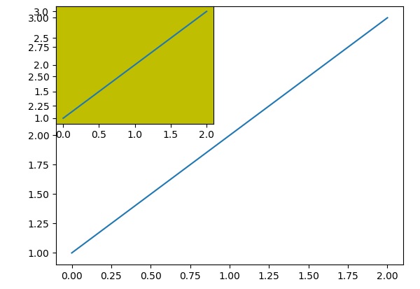
Функция add_subplot () класса figure не будет перезаписывать существующий график –
import matplotlib.pyplot as plt
fig = plt.figure()
ax1 = fig.add_subplot(111)
ax1.plot([1,2,3])
ax2 = fig.add_subplot(221, facecolor='y')
ax2.plot([1,2,3])
Когда приведенная выше строка кода выполняется, она генерирует следующий вывод –
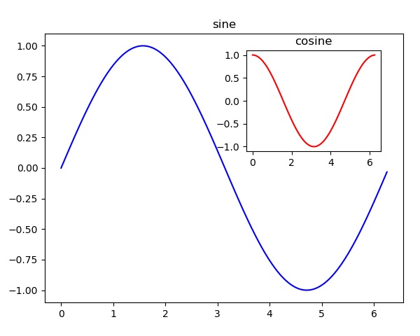
Вы можете добавить график вставки на том же рисунке, добавив другой объект осей на том же рисунке.
import matplotlib.pyplot as plt
import numpy as np
import math
x = np.arange(0, math.pi*2, 0.05)
fig=plt.figure()
axes1 = fig.add_axes([0.1, 0.1, 0.8, 0.8]) # main axes
axes2 = fig.add_axes([0.55, 0.55, 0.3, 0.3]) # inset axes
y = np.sin(x)
axes1.plot(x, y, 'b')
axes2.plot(x,np.cos(x),'r')
axes1.set_title('sine')
axes2.set_title("cosine")
plt.show()
После выполнения вышеупомянутой строки кода генерируется следующий вывод:
Matplotlib – Функция Subplots ()
API Pyplot в Matplotlib имеет вспомогательную функцию под названием subplots (), которая действует как служебная оболочка и помогает создавать общие макеты подзаговоров, включая объект фигуры, за один вызов.
Plt.subplots(nrows, ncols)
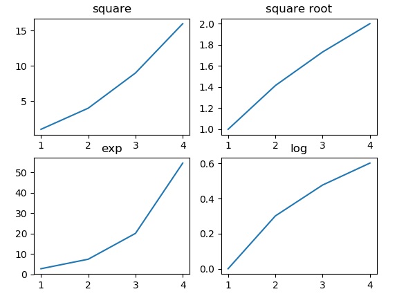
Два целочисленных аргумента этой функции задают количество строк и столбцов сетки подзаговоров. Функция возвращает объект фигурки и кортеж, содержащий объекты осей, равные nrows * ncols. Каждый объект оси доступен по его индексу. Здесь мы создаем участок из 2 строк по 2 столбца и отображаем 4 разных графика в каждом из них.
import matplotlib.pyplot as plt
fig,a =  plt.subplots(2,2)
import numpy as np
x = np.arange(1,5)
a[0][0].plot(x,x*x)
a[0][0].set_title('square')
a[0][1].plot(x,np.sqrt(x))
a[0][1].set_title('square root')
a[1][0].plot(x,np.exp(x))
a[1][0].set_title('exp')
a[1][1].plot(x,np.log10(x))
a[1][1].set_title('log')
plt.show()
Выше строка кода генерирует следующий вывод –
Функция Matplotlib – Subplot2grid ()
Эта функция дает больше гибкости при создании объекта осей в определенном месте сетки. Он также позволяет охватывать объект оси по нескольким строкам или столбцам.
Plt.subplot2grid(shape, location, rowspan, colspan)
В следующем примере сетка 3X3 объекта рисунка заполнена объектами осей различных размеров в интервалах строк и столбцов, каждый из которых показывает свой график.
import matplotlib.pyplot as plt
a1 = plt.subplot2grid((3,3),(0,0),colspan = 2)
a2 = plt.subplot2grid((3,3),(0,2), rowspan = 3)
a3 = plt.subplot2grid((3,3),(1,0),rowspan = 2, colspan = 2)
import numpy as np
x = np.arange(1,10)
a2.plot(x, x*x)
a2.set_title('square')
a1.plot(x, np.exp(x))
a1.set_title('exp')
a3.plot(x, np.log(x))
a3.set_title('log')
plt.tight_layout()
plt.show()
После выполнения вышеуказанного строкового кода генерируется следующий вывод:

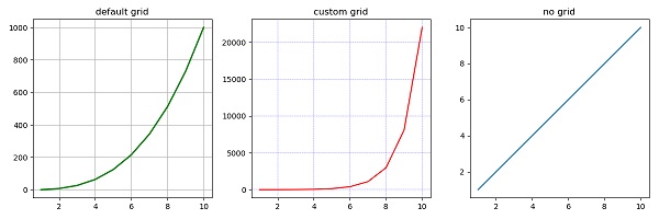
Матплотлиб – Сетки
Функция grid () объекта axes устанавливает или отключает видимость сетки внутри фигуры. Вы также можете отобразить основные / второстепенные (или оба) галочки сетки. Дополнительно свойства color, linestyle и linewidth могут быть установлены в функции grid ().
import matplotlib.pyplot as plt
import numpy as np
fig, axes = plt.subplots(1,3, figsize = (12,4))
x = np.arange(1,11)
axes[0].plot(x, x**3, 'g',lw=2)
axes[0].grid(True)
axes[0].set_title('default grid')
axes[1].plot(x, np.exp(x), 'r')
axes[1].grid(color='b', ls = '-.', lw = 0.25)
axes[1].set_title('custom grid')
axes[2].plot(x,x)
axes[2].set_title('no grid')
fig.tight_layout()
plt.show()
Matplotlib – Оси форматирования
Иногда одна или несколько точек намного больше, чем объем данных. В таком случае масштаб оси должен быть логарифмическим, а не нормальным. Это логарифмическая шкала. В Matplotlib это возможно, установив для свойства xscale или vscale объекта axes значение ‘log’.
Иногда требуется также показать некоторое дополнительное расстояние между номерами осей и меткой оси. Для свойства labelpad любой оси (x, y или обоих) можно установить желаемое значение.
Обе вышеуказанные функции демонстрируются с помощью следующего примера. Подплощадка справа имеет логарифмическую шкалу, а слева – ось x с меткой на большем расстоянии.
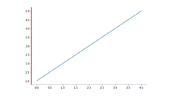
import matplotlib.pyplot as plt
import numpy as np
fig, axes = plt.subplots(1, 2, figsize=(10,4))
x = np.arange(1,5)
axes[0].plot( x, np.exp(x))
axes[0].plot(x,x**2)
axes[0].set_title("Normal scale")
axes[1].plot (x, np.exp(x))
axes[1].plot(x, x**2)
axes[1].set_yscale("log")
axes[1].set_title("Logarithmic scale (y)")
axes[0].set_xlabel("x axis")
axes[0].set_ylabel("y axis")
axes[0].xaxis.labelpad = 10
axes[1].set_xlabel("x axis")
axes[1].set_ylabel("y axis")
plt.show()

Оси осей – это линии, соединяющие отметки осей, обозначающие границы области графика. Объект оси имеет шипы, расположенные сверху, снизу, слева и справа.
Каждый позвоночник можно отформатировать, указав цвет и ширину. Любое ребро можно сделать невидимым, если его цвет не задан.
import matplotlib.pyplot as plt
fig = plt.figure()
ax = fig.add_axes([0,0,1,1])
ax.spines['bottom'].set_color('blue')
ax.spines['left'].set_color('red')
ax.spines['left'].set_linewidth(2)
ax.spines['right'].set_color(None)
ax.spines['top'].set_color(None)
ax.plot([1,2,3,4,5])
plt.show()
Matplotlib – установка пределов
Matplotlib автоматически достигает минимального и максимального значений переменных, которые будут отображаться вдоль осей x, y (и оси z в случае трехмерного графика). Однако можно установить ограничения явно с помощью функций set_xlim () и set_ylim () .
На следующем графике показаны автомасштабированные пределы осей x и y:
import matplotlib.pyplot as plt
fig = plt.figure()
a1 = fig.add_axes([0,0,1,1])
import numpy as np
x = np.arange(1,10)
a1.plot(x, np.exp(x))
a1.set_title('exp')
plt.show()
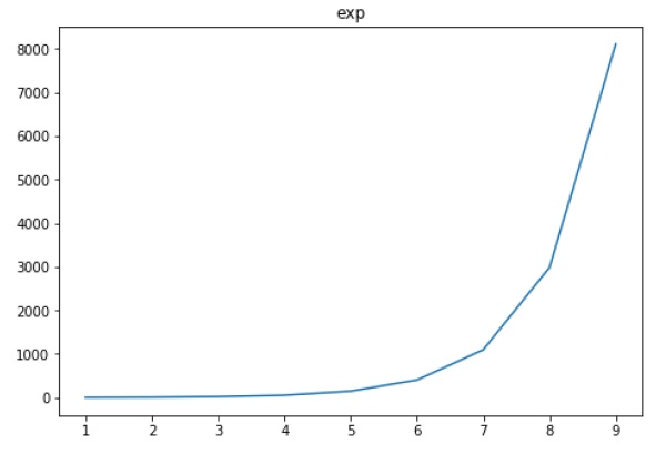
Теперь мы отформатируем пределы по оси х (от 0 до 10) и оси у (от 0 до 10000) –
import matplotlib.pyplot as plt
fig = plt.figure()
a1 = fig.add_axes([0,0,1,1])
import numpy as np
x = np.arange(1,10)
a1.plot(x, np.exp(x),'r')
a1.set_title('exp')
a1.set_ylim(0,10000)
a1.set_xlim(0,10)
plt.show()

Matplotlib – Установка меток и меток
Тики – это маркеры, обозначающие точки данных на осях. До сих пор Matplotlib – во всех наших предыдущих примерах – автоматически брал на себя задачу расстановки точек на оси. Стандартные локаторы и форматеры тиков Matplotlib спроектированы так, чтобы их было достаточно во многих распространенных ситуациях. Положение и метки галочек могут быть явно указаны в соответствии с конкретными требованиями.
Функция xticks () и yticks () принимает объект списка в качестве аргумента. Элементы в списке обозначают позиции на соответствующем действии, где будут отображаться галочки.
ax.set_xticks([2,4,6,8,10])
Этот метод помечает точки данных в заданных позициях галочками.
Аналогично, метки, соответствующие галочкам, могут быть установлены функциями set_xlabels () и set_ylabels () соответственно.
ax.set_xlabels([‘two’, ‘four’,’six’, ‘eight’, ‘ten’])
Это будет отображать текстовые метки под маркерами на оси х.
Следующий пример демонстрирует использование галочек и меток.
import matplotlib.pyplot as plt
import numpy as np
import math
x = np.arange(0, math.pi*2, 0.05)
fig = plt.figure()
ax = fig.add_axes([0.1, 0.1, 0.8, 0.8]) # main axes
y = np.sin(x)
ax.plot(x, y)
ax.set_xlabel(‘angle’)
ax.set_title('sine')
ax.set_xticks([0,2,4,6])
ax.set_xticklabels(['zero','two','four','six'])
ax.set_yticks([-1,0,1])
plt.show()

Matplotlib – Двойные Оси
Считается полезным иметь двойные оси x или y на фигуре. Более того, при построении кривых с различными единицами вместе. Matplotlib поддерживает это с помощью функций twinx и twiny.
В следующем примере график имеет двойные оси Y, одна из которых показывает exp (x), а другая – log (x) –
import matplotlib.pyplot as plt
import numpy as np
fig = plt.figure()
a1 = fig.add_axes([0,0,1,1])
x = np.arange(1,11)
a1.plot(x,np.exp(x))
a1.set_ylabel('exp')
a2 = a1.twinx()
a2.plot(x, np.log(x),'ro-')
a2.set_ylabel('log')
fig.legend(labels = ('exp','log'),loc='upper left')
plt.show()

Матплотлиб – Барный участок
Гистограмма или гистограмма – это диаграмма или диаграмма, которая представляет категориальные данные с прямоугольными столбцами с высотами или длинами, пропорциональными значениям, которые они представляют. Бары могут быть нанесены вертикально или горизонтально.
Гистограмма показывает сравнения между отдельными категориями. Одна ось диаграммы показывает конкретные категории, которые сравниваются, а другая ось представляет измеренное значение.
Matplotlib API предоставляет функцию bar (), которую можно использовать в стиле MATLAB, а также объектно-ориентированный API. Сигнатура функции bar () для использования с объектом axes выглядит следующим образом:
ax.bar(x, height, width, bottom, align)
Функция создает гистограмму со связанным прямоугольником размера (x-width = 2; x + width = 2; bottom; bottom + height).
Параметры для функции –
| Икс | последовательность скаляров, представляющих координаты х баров. выровняйте элементы управления, если x – центр полосы (по умолчанию) или левый край. |
| рост | скаляр или последовательность скаляров, представляющих высоту (и) столбцов. |
| ширина | скаляр или массив, необязательно. ширина (с) баров по умолчанию 0,8 |
| низ | скаляр или массив, необязательно. координаты y столбцов по умолчанию Нет. |
| выравнивать | {‘center’, ‘edge’}, необязательно, по умолчанию ‘center’ |
Функция возвращает контейнерный объект Matplotlib со всеми барами.
Ниже приведен простой пример графика бара Matplotlib. Показывает количество студентов, обучающихся на различных курсах, предлагаемых в институте.
import matplotlib.pyplot as plt
fig = plt.figure()
ax = fig.add_axes([0,0,1,1])
langs = ['C', 'C++', 'Java', 'Python', 'PHP']
students = [23,17,35,29,12]
ax.bar(langs,students)
plt.show()

При сравнении нескольких величин и при изменении одной переменной нам может потребоваться столбчатая диаграмма, на которой у нас есть столбцы одного цвета для одного количественного значения.
Мы можем построить несколько гистограмм, играя с толщиной и положением баров. Переменная данных содержит три ряда из четырех значений. Следующий скрипт покажет три гистограммы из четырех баров. Стержни будут иметь толщину 0,25 единиц. Каждая гистограмма будет сдвинута на 0,25 единицы от предыдущей. Объект данных представляет собой мультидикт, содержащий количество студентов, обучающихся в трех филиалах инженерного колледжа за последние четыре года.
import numpy as np
import matplotlib.pyplot as plt
data = [[30, 25, 50, 20],
[40, 23, 51, 17],
[35, 22, 45, 19]]
X = np.arange(4)
fig = plt.figure()
ax = fig.add_axes([0,0,1,1])
ax.bar(X + 0.00, data[0], color = 'b', width = 0.25)
ax.bar(X + 0.25, data[1], color = 'g', width = 0.25)
ax.bar(X + 0.50, data[2], color = 'r', width = 0.25)

Столбчатая диаграмма с накоплением объединяет столбцы, которые представляют разные группы друг над другом. Высота полученного столбца показывает объединенный результат групп.
Необязательный нижний параметр функции pyplot.bar () позволяет указать начальное значение для бара. Вместо того, чтобы работать от нуля до значения, оно будет идти снизу до значения. Первый вызов pyplot.bar () отображает синие полосы. Второй вызов pyplot.bar () отображает красные столбцы, причем нижняя часть синих столбцов находится сверху красных столбцов.
import numpy as np
import matplotlib.pyplot as plt
N = 5
menMeans = (20, 35, 30, 35, 27)
womenMeans = (25, 32, 34, 20, 25)
ind = np.arange(N) # the x locations for the groups
width = 0.35
fig = plt.figure()
ax = fig.add_axes([0,0,1,1])
ax.bar(ind, menMeans, width, color='r')
ax.bar(ind, womenMeans, width,bottom=menMeans, color='b')
ax.set_ylabel('Scores')
ax.set_title('Scores by group and gender')
ax.set_xticks(ind, ('G1', 'G2', 'G3', 'G4', 'G5'))
ax.set_yticks(np.arange(0, 81, 10))
ax.legend(labels=['Men', 'Women'])
plt.show()

Матплотлиб – Гистограмма
Гистограмма является точным представлением распределения числовых данных. Это оценка распределения вероятностей непрерывной переменной. Это своего рода гистограмма.
Чтобы построить гистограмму, выполните следующие действия.
- Бин диапазон значений.
- Разделите весь диапазон значений на ряд интервалов.
- Посчитайте, сколько значений попадают в каждый интервал.
Контейнеры обычно указываются как последовательные непересекающиеся интервалы переменной.
Функция matplotlib.pyplot.hist () строит гистограмму. Он вычисляет и рисует гистограмму х.
параметры
В следующей таблице перечислены параметры для гистограммы –
| Икс | массив или последовательность массивов |
| бункеры | целое число или последовательность или ‘auto’, необязательно |
| необязательные параметры | |
| спектр | Нижний и верхний диапазон бункеров. |
| плотность | Если True, первым элементом возвращаемого кортежа будет счет, нормализованный для формирования плотности вероятности. |
| кумулятивный | Если True, то гистограмма вычисляется, где каждый бин дает счетчики в этом бине, а также все бины для меньших значений. |
| histtype | Тип гистограммы для рисования. По умолчанию это «бар»
|
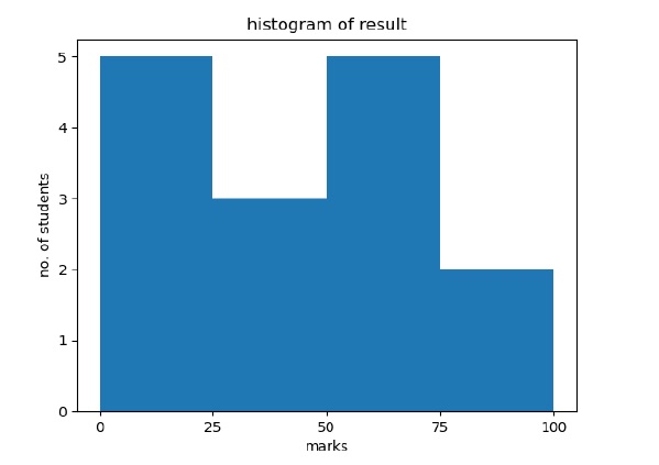
В следующем примере показана гистограмма оценок, полученных учениками в классе. Определены четыре ячейки: 0-25, 26-50, 51-75 и 76-100. Гистограмма показывает количество студентов, попадающих в этот диапазон.
from matplotlib import pyplot as plt
import numpy as np
fig,ax = plt.subplots(1,1)
a = np.array([22,87,5,43,56,73,55,54,11,20,51,5,79,31,27])
ax.hist(a, bins = [0,25,50,75,100])
ax.set_title("histogram of result")
ax.set_xticks([0,25,50,75,100])
ax.set_xlabel('marks')
ax.set_ylabel('no. of students')
plt.show()
Сюжет выглядит так, как показано ниже –
Matplotlib – круговая диаграмма
Круговая диаграмма может отображать только одну серию данных. Круговые диаграммы показывают размер элементов (называемых клином) в одном ряду данных, пропорциональный сумме элементов. Точки данных на круговой диаграмме отображаются в процентах от всей круговой диаграммы.
API Matplotlib имеет функцию pie (), которая генерирует круговую диаграмму, представляющую данные в массиве. Дробная площадь каждого клина определяется как x / sum (x) . Если сумма (х) <1, то значения х напрямую задают дробную площадь, и массив не будет нормализован. Результирующий пирог будет иметь пустой клин размером 1 – сумма (х).
Круговая диаграмма выглядит лучше всего, если фигура и оси имеют квадратную форму, или аспект оси совпадает.
параметры
В следующей таблице перечислены параметры для круговой диаграммы –
| Икс | массив типа. Размеры клина. |
| этикетки | список. Последовательность строк, обеспечивающая метки для каждого клина. |
| Цвета | Последовательность matplotlibcolorargs, через которую будет проходить круговая диаграмма. Если None, будет использовать цвета в текущем активном цикле. |
| Autopct | строка, используемая для обозначения клиньев их числовым значением. Метка будет размещена внутри клина. Строка формата будет fmt% pct. |
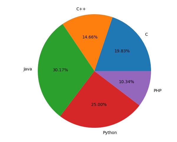
Следующий код использует функцию pie () для отображения круговой диаграммы в списке студентов, зачисленных на различные курсы компьютерного языка. Пропорциональный процент отображается внутри соответствующего клина с помощью параметра autopct, который установлен в% 1.2f%.
from matplotlib import pyplot as plt
import numpy as np
fig = plt.figure()
ax = fig.add_axes([0,0,1,1])
ax.axis('equal')
langs = ['C', 'C++', 'Java', 'Python', 'PHP']
students = [23,17,35,29,12]
ax.pie(students, labels = langs,autopct='%1.2f%%')
plt.show()
Matplotlib – Scatter Plot
Точечные диаграммы используются для построения точек данных по горизонтальной и вертикальной оси в попытке показать, насколько одна переменная подвержена влиянию другой. Каждая строка в таблице данных представлена маркером, положение которого зависит от его значений в столбцах, заданных по осям X и Y. Третья переменная может быть установлена, чтобы соответствовать цвету или размеру маркеров, таким образом добавляя еще одно измерение к графику.
Сценарий ниже показывает диаграмму разброса шкал оценок по сравнению с оценками мальчиков и девочек в двух разных цветах.
import matplotlib.pyplot as plt
girls_grades = [89, 90, 70, 89, 100, 80, 90, 100, 80, 34]
boys_grades = [30, 29, 49, 48, 100, 48, 38, 45, 20, 30]
grades_range = [10, 20, 30, 40, 50, 60, 70, 80, 90, 100]
fig=plt.figure()
ax=fig.add_axes([0,0,1,1])
ax.scatter(grades_range, girls_grades, color='r')
ax.scatter(grades_range, boys_grades, color='b')
ax.set_xlabel('Grades Range')
ax.set_ylabel('Grades Scored')
ax.set_title('scatter plot')
plt.show()

Матплотлиб – Контур Участок
Контурные графики (иногда называемые графиками уровня) – это способ показать трехмерную поверхность на двухмерной плоскости. Он отображает две прогнозирующие переменные XY на оси Y и ответную переменную Z в виде контуров. Эти контуры иногда называют z-слайсами или значениями изо-ответа.
Контурная диаграмма подходит, если вы хотите увидеть, как изменяется значение Z в зависимости от двух входов X и Y, так что Z = f (X, Y). Контурная линия или изолиния функции двух переменных – это кривая, вдоль которой функция имеет постоянное значение.
Независимые переменные x и y обычно ограничены регулярной сеткой, называемой meshgrid. Numpy.meshgrid создает прямоугольную сетку из массива значений x и массива значений y.
Matplotlib API содержит функции contour () и contourf (), которые рисуют контурные линии и закрашенные контуры соответственно. Обе функции нуждаются в трех параметрах x, y и z.
import numpy as np
import matplotlib.pyplot as plt
xlist = np.linspace(-3.0, 3.0, 100)
ylist = np.linspace(-3.0, 3.0, 100)
X, Y = np.meshgrid(xlist, ylist)
Z = np.sqrt(X**2 + Y**2)
fig,ax=plt.subplots(1,1)
cp = ax.contourf(X, Y, Z)
fig.colorbar(cp) # Add a colorbar to a plot
ax.set_title('Filled Contours Plot')
#ax.set_xlabel('x (cm)')
ax.set_ylabel('y (cm)')
plt.show()

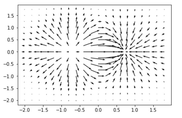
Matplotlib – Quiver Plot
На графике колчана векторы скорости отображаются в виде стрелок с компонентами (u, v) в точках (x, y).
quiver(x,y,u,v)
Приведенная выше команда отображает векторы в виде стрелок с координатами, указанными в каждой соответствующей паре элементов в x и y.
параметры
В следующей таблице перечислены различные параметры для графика колчана –
| Икс | 1D или 2D массив, последовательность. Координаты x расположения стрелок |
| Y | 1D или 2D массив, последовательность. Y координаты расположения стрелок |
| U | 1D или 2D массив, последовательность. Компоненты х векторов стрелок |
| v | 1D или 2D массив, последовательность. Компоненты y векторов стрелок |
| с | 1D или 2D массив, последовательность. Цвета стрелок |
Следующий код рисует простой сюжет колчана –
import matplotlib.pyplot as plt
import numpy as np
x,y = np.meshgrid(np.arange(-2, 2, .2), np.arange(-2, 2, .25))
z = x*np.exp(-x**2 - y**2)
v, u = np.gradient(z, .2, .2)
fig, ax = plt.subplots()
q = ax.quiver(x,y,u,v)
plt.show()
Matplotlib – Box Plot
Квадратный график, также известный как график с усами, отображает сводку данных, содержащих минимум, первый квартиль, медиану, третий квартиль и максимум. На графике прямоугольника мы рисуем прямоугольник от первого квартиля до третьего квартиля. Вертикальная линия проходит через прямоугольник на медиане. Усы идут от каждого квартиля до минимума или максимума.

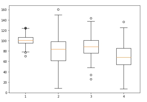
Давайте создадим данные для боксов. Мы используем функцию numpy.random.normal () для создания поддельных данных. Требуется три аргумента, среднее значение и стандартное отклонение нормального распределения, а также количество требуемых значений.
np.random.seed(10)
collectn_1 = np.random.normal(100, 10, 200)
collectn_2 = np.random.normal(80, 30, 200)
collectn_3 = np.random.normal(90, 20, 200)
collectn_4 = np.random.normal(70, 25, 200)
Список массивов, который мы создали выше, является единственным обязательным входом для создания боксплота. Используя строку кода data_to_plot , мы можем создать блокпост с помощью следующего кода:
fig = plt.figure()
# Create an axes instance
ax = fig.add_axes([0,0,1,1])
# Create the boxplot
bp = ax.boxplot(data_to_plot)
plt.show()
Выше строка кода будет генерировать следующий вывод –
Матплотлиб – Сюжет для скрипки
Графики для скрипки аналогичны блочным диаграммам, за исключением того, что они также показывают плотность вероятности данных при различных значениях. Эти графики включают маркер для медианы данных и прямоугольник, указывающий межквартильный диапазон, как на стандартных прямоугольниках. На этой рамке приведена оценка плотности ядра. Как и блочные графики, графики скрипки используются для представления сравнения переменного распределения (или выборочного распределения) по различным «категориям».
Сюжет для скрипки более информативен, чем простой сюжет. Фактически, в то время как на рамочном графике показаны только сводные статистические данные, такие как среднее / среднее и межквартильный диапазоны, на графике скрипки показано полное распределение данных.
 импортировать matplotlib.pyplot как plt

 np.random.seed (10)
 collectn_1 = np.random.normal (100, 10, 200)
 collectn_2 = np.random.normal (80, 30, 200)
 collectn_3 = np.random.normal (90, 20, 200)
 collectn_4 = np.random.normal (70, 25, 200)

 ## объединить эти разные коллекции в список
 data_to_plot = [collectn_1, collectn_2, collectn_3, collectn_4]

 # Создать экземпляр фигуры
 fig = plt.figure ()

 # Создать экземпляр оси
 ax = fig.add_axes ([0,0,1,1])

 # Создайте блокпост
 bp = ax.violinplot (data_to_plot)
 plt.show ()

Matplotlib – трехмерное черчение
Несмотря на то, что Matplotlib изначально разрабатывался с учетом только двумерного изображения, некоторые утилиты для трехмерного построения были построены поверх двумерного дисплея Matplotlib в более поздних версиях, чтобы обеспечить набор инструментов для визуализации трехмерных данных. Трехмерные графики активируются путем импорта набора инструментов mplot3d , включенного в пакет Matplotlib.
Трехмерные оси можно создать, передав ключевое слово projection = ‘3d’ любой из стандартных процедур создания осей.
from mpl_toolkits import mplot3d
import numpy as np
import matplotlib.pyplot as plt
fig = plt.figure()
ax = plt.axes(projection='3d')
z = np.linspace(0, 1, 100)
x = z * np.sin(20 * z)
y = z * np.cos(20 * z)
ax.plot3D(x, y, z, 'gray')
ax.set_title('3D line plot')
plt.show()
Теперь мы можем строить различные трехмерные типы графиков. Самым простым трехмерным графиком является трехмерный линейный график, созданный из наборов (x, y, z) троек. Это можно создать с помощью функции ax.plot3D.

Трехмерный график рассеяния создается с помощью функции ax.scatter3D .
from mpl_toolkits import mplot3d
import numpy as np
import matplotlib.pyplot as plt
fig = plt.figure()
ax = plt.axes(projection='3d')
z = np.linspace(0, 1, 100)
x = z * np.sin(20 * z)
y = z * np.cos(20 * z)
c = x + y
ax.scatter(x, y, z, c=c)
ax.set_title('3d Scatter plot')
plt.show()

Matplotlib – 3D Contour Plot
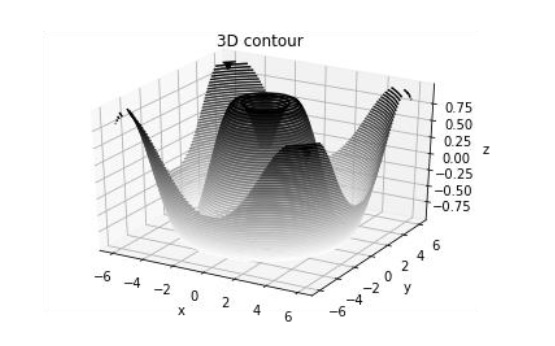
Функция ax.contour3D () создает трехмерный контурный график. Требуется, чтобы все входные данные были в форме двумерных регулярных сеток, а Z-данные оценивались в каждой точке. Здесь мы покажем трехмерную контурную диаграмму трехмерной синусоидальной функции.
from mpl_toolkits import mplot3d
import numpy as np
import matplotlib.pyplot as plt
def f(x, y):
   return np.sin(np.sqrt(x ** 2 + y ** 2))

x = np.linspace(-6, 6, 30)
y = np.linspace(-6, 6, 30)

X, Y = np.meshgrid(x, y)
Z = f(X, Y)

fig = plt.figure()
ax = plt.axes(projection='3d')
ax.contour3D(X, Y, Z, 50, cmap='binary')
ax.set_xlabel('x')
ax.set_ylabel('y')
ax.set_zlabel('z')
ax.set_title('3D contour')
plt.show()
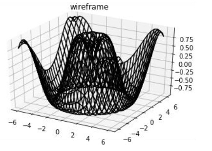
Matplotlib – 3D каркасный сюжет
Каркасный график принимает сетку значений и проецирует ее на указанную трехмерную поверхность, что позволяет довольно легко визуализировать получающиеся трехмерные формы. Функция plot_wireframe () используется для этой цели –
from mpl_toolkits import mplot3d
import numpy as np
import matplotlib.pyplot as plt
def f(x, y):
   return np.sin(np.sqrt(x ** 2 + y ** 2))

x = np.linspace(-6, 6, 30)
y = np.linspace(-6, 6, 30)

X, Y = np.meshgrid(x, y)
Z = f(X, Y)

fig = plt.figure()
ax = plt.axes(projection='3d')
ax.plot_wireframe(X, Y, Z, color='black')
ax.set_title('wireframe')
plt.show()
Выше строка кода будет генерировать следующий вывод –
Matplotlib – 3D Поверхностный сюжет
Поверхностный график показывает функциональную взаимосвязь между назначенной зависимой переменной (Y) и двумя независимыми переменными (X и Z). Сюжет является сопутствующим сюжетом для контурного сюжета. Поверхностный график похож на каркасный график, но каждая грань каркаса представляет собой заполненный многоугольник. Это может помочь восприятию топологии визуализируемой поверхности. Plot_surface () функции x, y и z в качестве аргументов.
from mpl_toolkits import mplot3d
import numpy as np
import matplotlib.pyplot as plt
x = np.outer(np.linspace(-2, 2, 30), np.ones(30))
y = x.copy().T # transpose
z = np.cos(x ** 2 + y ** 2)

fig = plt.figure()
ax = plt.axes(projection='3d')

ax.plot_surface(x, y, z,cmap='viridis', edgecolor='none')
ax.set_title('Surface plot')
plt.show()
Выше строка кода будет генерировать следующий вывод –

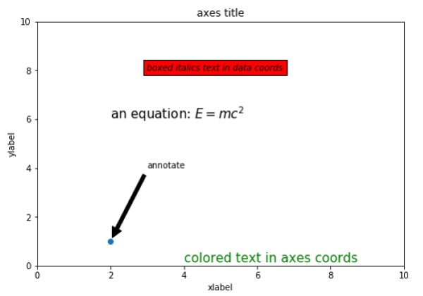
Matplotlib – Работа с текстом
Matplotlib имеет обширную текстовую поддержку, включая поддержку математических выражений, поддержку TrueType для растровых и векторных выводов, разделенный новой строкой текст с произвольными поворотами и поддержку юникода. Matplotlib включает в себя собственный matplotlib.font_manager, который реализует кросс-платформенный, W3C-совместимый алгоритм поиска шрифтов.
Пользователь имеет большой контроль над свойствами текста (размер шрифта, вес шрифта, расположение и цвет текста и т. Д.). Matplotlib реализует большое количество математических символов и команд TeX.
Следующий список команд используется для создания текста в интерфейсе Pyplot –
| текст | Добавить текст в произвольном месте осей. |
| аннотировать | Добавьте аннотацию с необязательной стрелкой в произвольном расположении осей. |
| xlabel | Добавьте метку к оси X осей. |
| ylabel | Добавьте метку к оси Y осей. |
| заглавие | Добавьте заголовок к Оси. |
| figtext | Добавьте текст в произвольном месте рисунка. |
| suptitle | Добавьте заголовок к рисунку. |
Все эти функции создают и возвращают экземпляр matplotlib.text.Text () .
Следующие сценарии демонстрируют использование некоторых из вышеуказанных функций –
import matplotlib.pyplot as plt
fig = plt.figure()

ax = fig.add_axes([0,0,1,1])

ax.set_title('axes title')
ax.set_xlabel('xlabel')
ax.set_ylabel('ylabel')
ax.text(3, 8, 'boxed italics text in data coords', style='italic',
bbox = {'facecolor': 'red'})
ax.text(2, 6, r'an equation: $E = mc^2$', fontsize = 15)
ax.text(4, 0.05, 'colored text in axes coords',
verticalalignment = 'bottom', color = 'green', fontsize = 15)
ax.plot([2], [1], 'o')
ax.annotate('annotate', xy = (2, 1), xytext = (3, 4),
arrowprops = dict(facecolor = 'black', shrink = 0.05))
ax.axis([0, 10, 0, 10])
plt.show()
Выше строка кода будет генерировать следующий вывод –
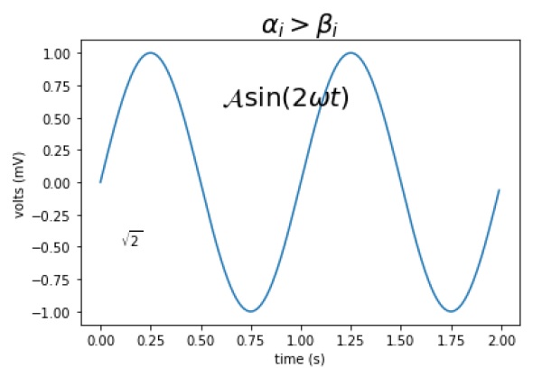
Matplotlib – математические выражения
Вы можете использовать подмножество TeXmarkup в любой текстовой строке Matplotlib, поместив ее внутри пары знаков доллара ($).
# math text
plt.title(r'$alpha > beta$')
Для создания нижних и верхних индексов используйте символы «_» и «^» –
r'$alpha_i> beta_i$'

import numpy as np
import matplotlib.pyplot as plt
t = np.arange(0.0, 2.0, 0.01)
s = np.sin(2*np.pi*t)

plt.plot(t,s)
plt.title(r'$alpha_i> beta_i$', fontsize=20)

plt.text(0.6, 0.6, r'$mathcal{A}mathrm{sin}(2 omega t)$', fontsize = 20)
plt.text(0.1, -0.5, r'$sqrt{2}$', fontsize=10)
plt.xlabel('time (s)')
plt.ylabel('volts (mV)')
plt.show()
Выше строка кода будет генерировать следующий вывод –
Matplotlib – Работа с изображениями
Модуль изображения в пакете Matplotlib предоставляет функции, необходимые для загрузки, изменения масштаба и отображения изображения.
Загрузка данных изображения поддерживается библиотекой Pillow. Собственно, Matplotlib поддерживает только изображения PNG. Команды, показанные ниже, возвращаются к Подушке, если не удается выполнить родное чтение.
Изображение, используемое в этом примере, является файлом PNG, но имейте это в виду требование подушки для ваших собственных данных. Функция imread () используется для чтения данных изображения в объекте ndarray типа float32 dtype.
import matplotlib.pyplot as plt
import matplotlib.image as mpimg
import numpy as np
img = mpimg.imread('mtplogo.png')
Предполагая, что следующее изображение с именем mtplogo.png присутствует в текущем рабочем каталоге.

Любой массив, содержащий данные изображения, можно сохранить в файл на диске, выполнив функцию imsave () . Здесь вертикально перевернутая версия оригинального png-файла сохраняется путем задания параметра origin как более низкого.
plt.imsave("logo.png", img, cmap = 'gray', origin = 'lower')
Новое изображение отображается, как показано ниже, если оно открыто в любой программе просмотра изображений.

Чтобы нарисовать изображение в программе просмотра Matplotlib, выполните функцию imshow () .
imgplot = plt.imshow(img)
Матплотлиб – Преобразования
Пакет matplotlib построен поверх структуры преобразования, чтобы легко перемещаться между системами координат. Можно использовать четыре системы координат. Системы кратко описаны в таблице, приведенной ниже –
| координировать | Объект трансформации | Описание |
|---|---|---|
| Данные | ax.transData |
Пользовательская система данных о земле. контролируется xlim и ylim |
| Топоры | ax.transAxes |
Система координат осей. (0,0) слева внизу и (1,1) справа вверху от осей. |
| фигура | fig.transFigure |
Система координат рисунка. (0,0) слева внизу и (1,1) вверху справа на рисунке |
| дисплей | Никто |
Это пиксельная система координат дисплея. (0,0) – левый нижний угол, а (ширина, высота) – верхний правый угол экрана в пикселях. Альтернативно, (matplotlib.transforms.IdentityTransform ()) может использоваться вместо None. |
Пользовательская система данных о земле. контролируется xlim и ylim
Система координат осей. (0,0) слева внизу и (1,1) справа вверху от осей.
Система координат рисунка. (0,0) слева внизу и (1,1) вверху справа на рисунке
Это пиксельная система координат дисплея. (0,0) – левый нижний угол, а (ширина, высота) – верхний правый угол экрана в пикселях.
Альтернативно, (matplotlib.transforms.IdentityTransform ()) может использоваться вместо None.
Рассмотрим следующий пример –
axes.text(x,y,"my label")
Текст размещается в теоретической позиции точки данных (x, y). Таким образом, мы будем говорить о «координатах данных».
Используя другие объекты трансформации, размещение можно контролировать. Например, если вышеуказанный тест должен быть помещен в систему координат центра осей, выполните следующую строку кода:
axes.text(0.5, 0.5, "middle of graph", transform=axes.transAxes)
Эти преобразования могут быть использованы для любого типа объектов Matplotlib. Преобразование по умолчанию для ax.text – это ax.transData, а преобразование по умолчанию для fig.text – это fig.transFigure.
Система координат осей чрезвычайно полезна при размещении текста на ваших осях. Вы можете часто хотеть текстовый пузырь в фиксированном месте; например, в левом верхнем углу панели осей, и это положение остается неизменным при панорамировании или масштабировании.
Matplotlib — Introduction
Matplotlib is one of the most popular Python packages used for data visualization. It is a cross-platform library for making 2D plots from data in arrays. Matplotlib is written in Python and makes use of NumPy, the numerical mathematics extension of Python. It provides an object-oriented API that helps in embedding plots in applications using Python GUI toolkits such as PyQt, WxPythonotTkinter. It can be used in Python and IPython shells, Jupyter notebook and web application servers also.
Matplotlib has a procedural interface named the Pylab, which is designed to resemble MATLAB, a proprietary programming language developed by MathWorks. Matplotlib along with NumPy can be considered as the open source equivalent of MATLAB.
Matplotlib was originally written by John D. Hunter in 2003. The current stable version is 2.2.0 released in January 2018.
Matplotlib — Environment Setup
Matplotlib and its dependency packages are available in the form of wheel packages on the standard Python package repositories and can be installed on Windows, Linux as well as MacOS systems using the pip package manager.
pip3 install matplotlib
Incase Python 2.7 or 3.4 versions are not installed for all users, the Microsoft Visual C++ 2008 (64 bit or 32 bit forPython 2.7) or Microsoft Visual C++ 2010 (64 bit or 32 bit for Python 3.4) redistributable packages need to be installed.
If you are using Python 2.7 on a Mac, execute the following command −
xcode-select –install
Upon execution of the above command, the subprocess32 — a dependency, may be compiled.
On extremely old versions of Linux and Python 2.7, you may need to install the master version of subprocess32.
Matplotlib requires a large number of dependencies −
- Python (>= 2.7 or >= 3.4)
- NumPy
- setuptools
- dateutil
- pyparsing
- libpng
- pytz
- FreeType
- cycler
- six
Optionally, you can also install a number of packages to enable better user interface toolkits.
- tk
- PyQt4
- PyQt5
- pygtk
- wxpython
- pycairo
- Tornado
For better support of animation output format and image file formats, LaTeX, etc., you can install the following −
- _mpeg/avconv
- ImageMagick
- Pillow (>=2.0)
- LaTeX and GhostScript (for rendering text with LaTeX).
- LaTeX and GhostScript (for rendering text with LaTeX).
Matplotlib — Anaconda distribution
Anaconda is a free and open source distribution of the Python and R programming languages for large-scale data processing, predictive analytics, and scientific computing. The distribution makes package management and deployment simple and easy. Matplotlib and lots of other useful (data) science tools form part of the distribution. Package versions are managed by the package management system Conda. The advantage of Anaconda is that you have access to over 720 packages that can easily be installed with Anaconda’s Conda, a package, dependency, and environment manager.
Anaconda distribution is available for installation at https://www.anaconda.com/download/. For installation on Windows, 32 and 64 bit binaries are available −
https://repo.continuum.io/archive/Anaconda3-5.1.0-Windows-x86.exe
https://repo.continuum.io/archive/Anaconda3-5.1.0-Windows-x86_64.exe
Installation is a fairly straightforward wizard based process. You can choose between adding Anaconda in PATH variable and registering Anaconda as your default Python.
For installation on Linux, download installers for 32 bit and 64 bit installers from the downloads page −
https://repo.continuum.io/archive/Anaconda3-5.1.0-Linux-x86.sh
https://repo.continuum.io/archive/Anaconda3-5.1.0-Linux-x86_64.sh
Now, run the following command from the Linux terminal −
$ bash Anaconda3-5.0.1-Linux-x86_64.sh
Canopy and ActiveState are the most sought after choices for Windows, macOS and common Linux platforms. The Windows users can find an option in WinPython.
Matplotlib — Jupyter Notebook
Jupyter is a loose acronym meaning Julia, Python, and R. These programming languages were the first target languages of the Jupyter application, but nowadays, the notebook technology also supports many other languages.
In 2001, Fernando Pérez started developing Ipython. IPython is a command shell for interactive computing in multiple programming languages, originally developed for the Python.
Consider the following features provided by IPython −
-
Interactive shells (terminal and Qt-based).
-
A browser-based notebook with support for code, text, mathematical expressions, inline plots and other media.
-
Support for interactive data visualization and use of GUI toolkits.
-
Flexible, embeddable interpreters to load into one’s own projects.
In 2014, Fernando Pérez announced a spin-off project from IPython called Project Jupyter. IPython will continue to exist as a Python shell and a kernel for Jupyter, while the notebook and other language-agnostic parts of IPython will move under the Jupyter name. Jupyter added support for Julia, R, Haskell and Ruby.
To start the Jupyter notebook, open Anaconda navigator (a desktop graphical user interface included in Anaconda that allows you to launch applications and easily manage Conda packages, environments and channels without the need to use command line commands).
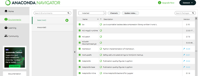
Navigator displays the installed components in the distribution.

Launch Jupyter Notebook from the Navigator −

You will see the application opening in the web browser on the following address − http://localhost:8888.
You probably want to start by making a new notebook. You can easily do this by clicking on the «New button» in the «Files tab». You see that you have the option to make a regular text file, a folder, and a terminal. Lastly, you will also see the option to make a Python 3 notebook.

Matplotlib — Pyplot API
A new untitled notebook with the .ipynbextension (stands for the IPython notebook) is displayed in the new tab of the browser.
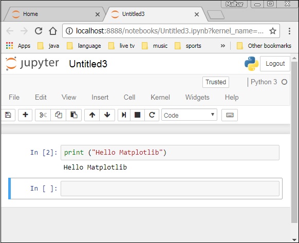
matplotlib.pyplot is a collection of command style functions that make Matplotlib work like MATLAB. Each Pyplot function makes some change to a figure. For example, a function creates a figure, a plotting area in a figure, plots some lines in a plotting area, decorates the plot with labels, etc.
Types of Plots
| Sr.No | Function & Description |
|---|---|
| 1 |
Bar Make a bar plot. |
| 2 |
Barh Make a horizontal bar plot. |
| 3 |
Boxplot Make a box and whisker plot. |
| 4 |
Hist Plot a histogram. |
| 5 |
hist2d Make a 2D histogram plot. |
| 6 |
Pie Plot a pie chart. |
| 7 |
Plot Plot lines and/or markers to the Axes. |
| 8 |
Polar Make a polar plot.. |
| 9 |
Scatter Make a scatter plot of x vs y. |
| 10 |
Stackplot Draws a stacked area plot. |
| 11 |
Stem Create a stem plot. |
| 12 |
Step Make a step plot. |
| 13 |
Quiver Plot a 2-D field of arrows. |
Image Functions
| Sr.No | Function & Description |
|---|---|
| 1 |
Imread Read an image from a file into an array. |
| 2 |
Imsave Save an array as in image file. |
| 3 |
Imshow Display an image on the axes. |
Axis Functions
| Sr.No | Function & Description |
|---|---|
| 1 |
Axes Add axes to the figure. |
| 2 |
Text Add text to the axes. |
| 3 |
Title Set a title of the current axes. |
| 4 |
Xlabel Set the x axis label of the current axis. |
| 5 |
Xlim Get or set the x limits of the current axes. |
| 6 |
Xscale . |
| 7 |
Xticks Get or set the x-limits of the current tick locations and labels. |
| 8 |
Ylabel Set the y axis label of the current axis. |
| 9 |
Ylim Get or set the y-limits of the current axes. |
| 10 |
Yscale Set the scaling of the y-axis. |
| 11 |
Yticks Get or set the y-limits of the current tick locations and labels. |
Figure Functions
| Sr.No | Function & Description |
|---|---|
| 1 |
Figtext Add text to figure. |
| 2 |
Figure Creates a new figure. |
| 3 |
Show Display a figure. |
| 4 |
Savefig Save the current figure. |
| 5 |
Close Close a figure window. |
Matplotlib — Simple Plot
In this chapter, we will learn how to create a simple plot with Matplotlib.
We shall now display a simple line plot of angle in radians vs. its sine value in Matplotlib. To begin with, the Pyplot module from Matplotlib package is imported, with an alias plt as a matter of convention.
import matplotlib.pyplot as plt
Next we need an array of numbers to plot. Various array functions are defined in the NumPy library which is imported with the np alias.
import numpy as np
We now obtain the ndarray object of angles between 0 and 2π using the arange() function from the NumPy library.
x = np.arange(0, math.pi*2, 0.05)
The ndarray object serves as values on x axis of the graph. The corresponding sine values of angles in x to be displayed on y axis are obtained by the following statement −
y = np.sin(x)
The values from two arrays are plotted using the plot() function.
plt.plot(x,y)
You can set the plot title, and labels for x and y axes.
You can set the plot title, and labels for x and y axes.
plt.xlabel("angle")
plt.ylabel("sine")
plt.title('sine wave')
The Plot viewer window is invoked by the show() function −
plt.show()
The complete program is as follows −
from matplotlib import pyplot as plt
import numpy as np
import math #needed for definition of pi
x = np.arange(0, math.pi*2, 0.05)
y = np.sin(x)
plt.plot(x,y)
plt.xlabel("angle")
plt.ylabel("sine")
plt.title('sine wave')
plt.show()
When the above line of code is executed, the following graph is displayed −
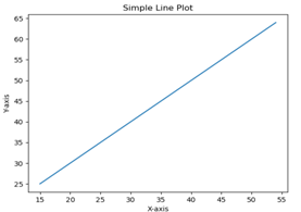
Now, use the Jupyter notebook with Matplotlib.
Launch the Jupyter notebook from Anaconda navigator or command line as described earlier. In the input cell, enter import statements for Pyplot and NumPy −
from matplotlib import pyplot as plt
import numpy as np
To display plot outputs inside the notebook itself (and not in the separate viewer), enter the following magic statement −
%matplotlib inline
Obtain x as the ndarray object containing angles in radians between 0 to 2π, and y as sine value of each angle −
import math
x = np.arange(0, math.pi*2, 0.05)
y = np.sin(x)
Set labels for x and y axes as well as the plot title −
plt.xlabel("angle")
plt.ylabel("sine")
plt.title('sine wave')
Finally execute the plot() function to generate the sine wave display in the notebook (no need to run the show() function) −
plt.plot(x,y)
After the execution of the final line of code, the following output is displayed −
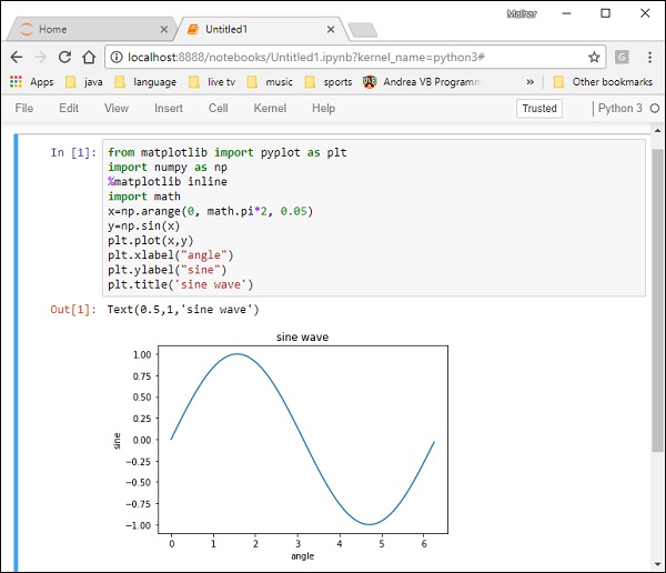
Matplotlib — PyLab module
PyLab is a procedural interface to the Matplotlib object-oriented plotting library. Matplotlib is the whole package; matplotlib.pyplot is a module in Matplotlib; and PyLab is a module that gets installed alongside Matplotlib.
PyLab is a convenience module that bulk imports matplotlib.pyplot (for plotting) and NumPy (for Mathematics and working with arrays) in a single name space. Although many examples use PyLab, it is no longer recommended.
Basic Plotting
Plotting curves is done with the plot command. It takes a pair of same-length arrays (or sequences) −
from numpy import *
from pylab import *
x = linspace(-3, 3, 30)
y = x**2
plot(x, y)
show()
The above line of code generates the following output −
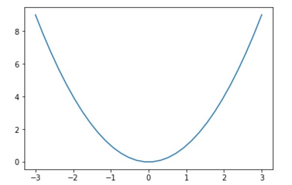
To plot symbols rather than lines, provide an additional string argument.
| symbols | — , –, -., , . , , , o , ^ , v , < , > , s , + , x , D , d , 1 , 2 , 3 , 4 , h , H , p , | , _ |
| colors | b, g, r, c, m, y, k, w |
Now, consider executing the following code −
from pylab import *
x = linspace(-3, 3, 30)
y = x**2
plot(x, y, 'r.')
show()
It plots the red dots as shown below −
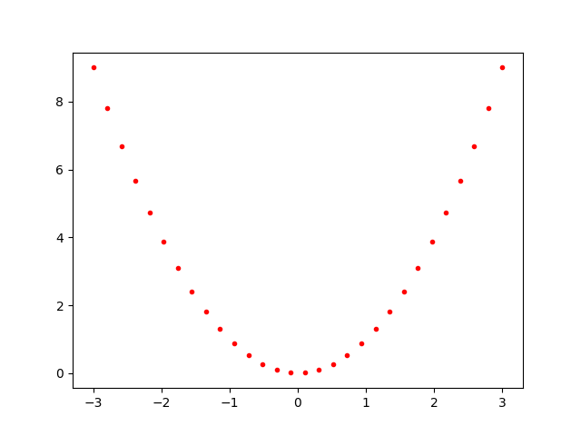
Plots can be overlaid. Just use the multiple plot commands. Use clf() to clear the plot.
from pylab import *
plot(x, sin(x))
plot(x, cos(x), 'r-')
plot(x, -sin(x), 'g--')
show()
The above line of code generates the following output −
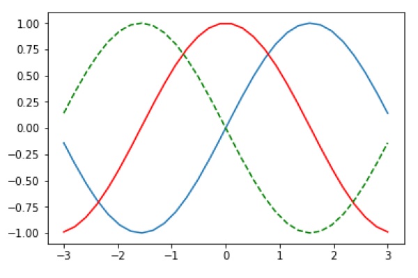
Matplotlib — Object-oriented Interface
While it is easy to quickly generate plots with the matplotlib.pyplot module, the use of object-oriented approach is recommended as it gives more control and customization of your plots. Most of the functions are also available in the
matplotlib.axes.Axes class.
The main idea behind using the more formal object-oriented method is to create figure objects and then just call methods or attributes off of that object. This approach helps better in dealing with a canvas that has multiple plots on it.
In object-oriented interface, Pyplot is used only for a few functions such as figure creation, and the user explicitly creates and keeps track of the figure and axes objects. At this level, the user uses Pyplot to create figures, and through those figures, one or more axes objects can be created. These axes objects are then used for most plotting actions.
To begin with, we create a figure instance which provides an empty canvas.
fig = plt.figure()
Now add axes to figure. The add_axes() method requires a list object of 4 elements corresponding to left, bottom, width and height of the figure. Each number must be between 0 and 1 −
ax=fig.add_axes([0,0,1,1])
Set labels for x and y axis as well as title −
ax.set_title("sine wave")
ax.set_xlabel('angle')
ax.set_ylabel('sine')
Invoke the plot() method of the axes object.
ax.plot(x,y)
If you are using Jupyter notebook, the %matplotlib inline directive has to be issued; the otherwistshow() function of pyplot module displays the plot.
Consider executing the following code −
from matplotlib import pyplot as plt
import numpy as np
import math
x = np.arange(0, math.pi*2, 0.05)
y = np.sin(x)
fig = plt.figure()
ax = fig.add_axes([0,0,1,1])
ax.plot(x,y)
ax.set_title("sine wave")
ax.set_xlabel('angle')
ax.set_ylabel('sine')
plt.show()
Output
The above line of code generates the following output −
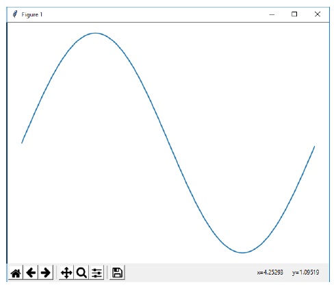
The same code when run in Jupyter notebook shows the output as shown below −
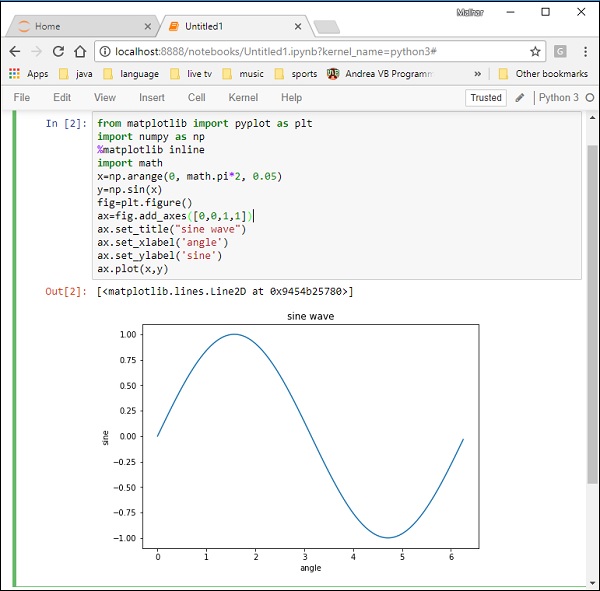
Matplotlib — Figure Class
The matplotlib.figure module contains the Figure class. It is a top-level container for all plot elements. The Figure object is instantiated by calling the figure() function from the pyplot module −
fig = plt.figure()
The following table shows the additional parameters −
| Figsize | (width,height) tuple in inches |
| Dpi | Dots per inches |
| Facecolor | Figure patch facecolor |
| Edgecolor | Figure patch edge color |
| Linewidth | Edge line width |
Matplotlib — Axes Class
Axes object is the region of the image with the data space. A given figure can contain many Axes, but a given Axes object can only be in one Figure. The Axes contains two (or three in the case of 3D) Axis objects. The Axes class and its member functions are the primary entry point to working with the OO interface.
Axes object is added to figure by calling the add_axes() method. It returns the axes object and adds an axes at position rect [left, bottom, width, height] where all quantities are in fractions of figure width and height.
Parameter
Following is the parameter for the Axes class −
-
rect − A 4-length sequence of [left, bottom, width, height] quantities.
ax=fig.add_axes([0,0,1,1])
The following member functions of axes class add different elements to plot −
Legend
The legend() method of axes class adds a legend to the plot figure. It takes three parameters −
ax.legend(handles, labels, loc)
Where labels is a sequence of strings and handles a sequence of Line2D or Patch instances. loc can be a string or an integer specifying the legend location.
| Location string | Location code |
|---|---|
| Best | 0 |
| upper right | 1 |
| upper left | 2 |
| lower left | 3 |
| lower right | 4 |
| Right | 5 |
| Center left | 6 |
| Center right | 7 |
| lower center | 8 |
| upper center | 9 |
| Center | 10 |
axes.plot()
This is the basic method of axes class that plots values of one array versus another as lines or markers. The plot() method can have an optional format string argument to specify color, style and size of line and marker.
Color codes
| Character | Color |
|---|---|
| ‘b’ | Blue |
| ‘g’ | Green |
| ‘r’ | Red |
| ‘b’ | Blue |
| ‘c’ | Cyan |
| ‘m’ | Magenta |
| ‘y’ | Yellow |
| ‘k’ | Black |
| ‘b’ | Blue |
| ‘w’ | White |
Marker codes
| Character | Description |
|---|---|
| ‘.’ | Point marker |
| ‘o’ | Circle marker |
| ‘x’ | X marker |
| ‘D’ | Diamond marker |
| ‘H’ | Hexagon marker |
| ‘s’ | Square marker |
| ‘+’ | Plus marker |
Line styles
| Character | Description |
|---|---|
| ‘-‘ | Solid line |
| ‘—‘ | Dashed line |
| ‘-.’ | Dash-dot line |
| ‘:’ | Dotted line |
| ‘H’ | Hexagon marker |
Following example shows the advertisement expenses and sales figures of TV and smartphone in the form of line plots. Line representing TV is a solid line with yellow colour and square markers whereas smartphone line is a dashed line with green colour and circle marker.
import matplotlib.pyplot as plt
y = [1, 4, 9, 16, 25,36,49, 64]
x1 = [1, 16, 30, 42,55, 68, 77,88]
x2 = [1,6,12,18,28, 40, 52, 65]
fig = plt.figure()
ax = fig.add_axes([0,0,1,1])
l1 = ax.plot(x1,y,'ys-') # solid line with yellow colour and square marker
l2 = ax.plot(x2,y,'go--') # dash line with green colour and circle marker
ax.legend(labels = ('tv', 'Smartphone'), loc = 'lower right') # legend placed at lower right
ax.set_title("Advertisement effect on sales")
ax.set_xlabel('medium')
ax.set_ylabel('sales')
plt.show()
When the above line of code is executed, it produces the following plot −
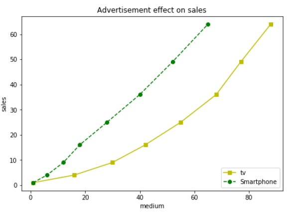
Matplotlib — Multiplots
In this chapter, we will learn how to create multiple subplots on same canvas.
The subplot() function returns the axes object at a given grid position. The Call signature of this function is −
plt.subplot(subplot(nrows, ncols, index)
In the current figure, the function creates and returns an Axes object, at position index of a grid of nrows by ncolsaxes. Indexes go from 1 to nrows * ncols, incrementing in row-major order.Ifnrows, ncols and index are all less than 10. The indexes can also be given as single, concatenated, threedigitnumber.
For example, subplot(2, 3, 3) and subplot(233) both create an Axes at the top right corner of the current figure, occupying half of the figure height and a third of the figure width.
Creating a subplot will delete any pre-existing subplot that overlaps with it beyond sharing a boundary.
import matplotlib.pyplot as plt
# plot a line, implicitly creating a subplot(111)
plt.plot([1,2,3])
# now create a subplot which represents the top plot of a grid with 2 rows and 1 column.
#Since this subplot will overlap the first, the plot (and its axes) previously
created, will be removed
plt.subplot(211)
plt.plot(range(12))
plt.subplot(212, facecolor='y') # creates 2nd subplot with yellow background
plt.plot(range(12))
The above line of code generates the following output −

The add_subplot() function of the figure class will not overwrite the existing plot −
import matplotlib.pyplot as plt
fig = plt.figure()
ax1 = fig.add_subplot(111)
ax1.plot([1,2,3])
ax2 = fig.add_subplot(221, facecolor='y')
ax2.plot([1,2,3])
When the above line of code is executed, it generates the following output −

You can add an insert plot in the same figure by adding another axes object in the same figure canvas.
import matplotlib.pyplot as plt
import numpy as np
import math
x = np.arange(0, math.pi*2, 0.05)
fig=plt.figure()
axes1 = fig.add_axes([0.1, 0.1, 0.8, 0.8]) # main axes
axes2 = fig.add_axes([0.55, 0.55, 0.3, 0.3]) # inset axes
y = np.sin(x)
axes1.plot(x, y, 'b')
axes2.plot(x,np.cos(x),'r')
axes1.set_title('sine')
axes2.set_title("cosine")
plt.show()
Upon execution of the above line of code, the following output is generated −

Matplotlib — Subplots() Function
Matplotlib’spyplot API has a convenience function called subplots() which acts as a utility wrapper and helps in creating common layouts of subplots, including the enclosing figure object, in a single call.
Plt.subplots(nrows, ncols)
The two integer arguments to this function specify the number of rows and columns of the subplot grid. The function returns a figure object and a tuple containing axes objects equal to nrows*ncols. Each axes object is accessible by its index. Here we create a subplot of 2 rows by 2 columns and display 4 different plots in each subplot.
import matplotlib.pyplot as plt
fig,a =  plt.subplots(2,2)
import numpy as np
x = np.arange(1,5)
a[0][0].plot(x,x*x)
a[0][0].set_title('square')
a[0][1].plot(x,np.sqrt(x))
a[0][1].set_title('square root')
a[1][0].plot(x,np.exp(x))
a[1][0].set_title('exp')
a[1][1].plot(x,np.log10(x))
a[1][1].set_title('log')
plt.show()
The above line of code generates the following output −

Matplotlib — Subplot2grid() Function
This function gives more flexibility in creating an axes object at a specific location of the grid. It also allows the axes object to be spanned across multiple rows or columns.
Plt.subplot2grid(shape, location, rowspan, colspan)
In the following example, a 3X3 grid of the figure object is filled with axes objects of varying sizes in row and column spans, each showing a different plot.
import matplotlib.pyplot as plt
a1 = plt.subplot2grid((3,3),(0,0),colspan = 2)
a2 = plt.subplot2grid((3,3),(0,2), rowspan = 3)
a3 = plt.subplot2grid((3,3),(1,0),rowspan = 2, colspan = 2)
import numpy as np
x = np.arange(1,10)
a2.plot(x, x*x)
a2.set_title('square')
a1.plot(x, np.exp(x))
a1.set_title('exp')
a3.plot(x, np.log(x))
a3.set_title('log')
plt.tight_layout()
plt.show()
Upon execution of the above line code, the following output is generated −
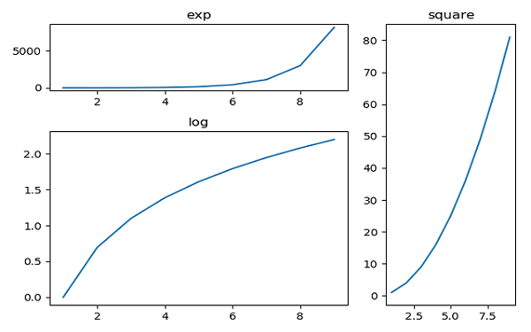
Matplotlib — Grids
The grid() function of axes object sets visibility of grid inside the figure to on or off. You can also display major / minor (or both) ticks of the grid. Additionally color, linestyle and linewidth properties can be set in the grid() function.
import matplotlib.pyplot as plt
import numpy as np
fig, axes = plt.subplots(1,3, figsize = (12,4))
x = np.arange(1,11)
axes[0].plot(x, x**3, 'g',lw=2)
axes[0].grid(True)
axes[0].set_title('default grid')
axes[1].plot(x, np.exp(x), 'r')
axes[1].grid(color='b', ls = '-.', lw = 0.25)
axes[1].set_title('custom grid')
axes[2].plot(x,x)
axes[2].set_title('no grid')
fig.tight_layout()
plt.show()
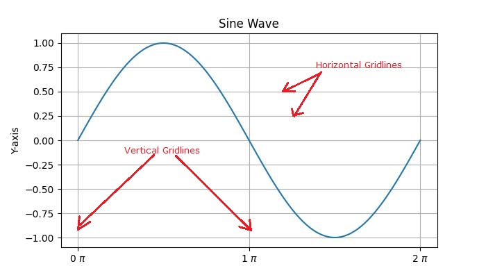
Matplotlib — Formatting Axes
Sometimes, one or a few points are much larger than the bulk of data. In such a case, the scale of an axis needs to be set as logarithmic rather than the normal scale. This is the Logarithmic scale. In Matplotlib, it is possible by setting xscale or vscale property of axes object to ‘log’.
It is also required sometimes to show some additional distance between axis numbers and axis label. The labelpad property of either axis (x or y or both) can be set to the desired value.
Both the above features are demonstrated with the help of the following example. The subplot on the right has a logarithmic scale and one on left has its x axis having label at more distance.
import matplotlib.pyplot as plt
import numpy as np
fig, axes = plt.subplots(1, 2, figsize=(10,4))
x = np.arange(1,5)
axes[0].plot( x, np.exp(x))
axes[0].plot(x,x**2)
axes[0].set_title("Normal scale")
axes[1].plot (x, np.exp(x))
axes[1].plot(x, x**2)
axes[1].set_yscale("log")
axes[1].set_title("Logarithmic scale (y)")
axes[0].set_xlabel("x axis")
axes[0].set_ylabel("y axis")
axes[0].xaxis.labelpad = 10
axes[1].set_xlabel("x axis")
axes[1].set_ylabel("y axis")
plt.show()
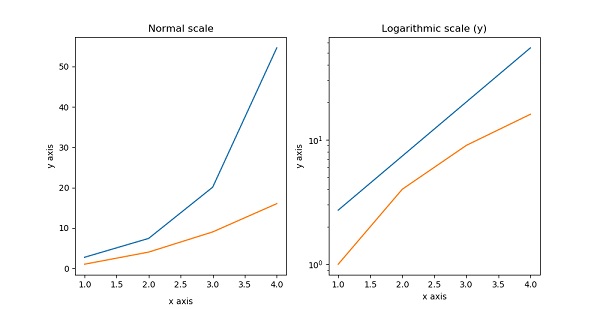
Axis spines are the lines connecting axis tick marks demarcating boundaries of plot area. The axes object has spines located at top, bottom, left and right.
Each spine can be formatted by specifying color and width. Any edge can be made invisible if its color is set to none.
import matplotlib.pyplot as plt
fig = plt.figure()
ax = fig.add_axes([0,0,1,1])
ax.spines['bottom'].set_color('blue')
ax.spines['left'].set_color('red')
ax.spines['left'].set_linewidth(2)
ax.spines['right'].set_color(None)
ax.spines['top'].set_color(None)
ax.plot([1,2,3,4,5])
plt.show()

Matplotlib — Setting Limits
Matplotlib automatically arrives at the minimum and maximum values of variables to be displayed along x, y (and z axis in case of 3D plot) axes of a plot. However, it is possible to set the limits explicitly by using set_xlim() and set_ylim() functions.
In the following plot, the autoscaled limits of x and y axes are shown −
import matplotlib.pyplot as plt
fig = plt.figure()
a1 = fig.add_axes([0,0,1,1])
import numpy as np
x = np.arange(1,10)
a1.plot(x, np.exp(x))
a1.set_title('exp')
plt.show()

Now we format the limits on x axis to (0 to 10) and y axis (0 to 10000) −
import matplotlib.pyplot as plt
fig = plt.figure()
a1 = fig.add_axes([0,0,1,1])
import numpy as np
x = np.arange(1,10)
a1.plot(x, np.exp(x),'r')
a1.set_title('exp')
a1.set_ylim(0,10000)
a1.set_xlim(0,10)
plt.show()
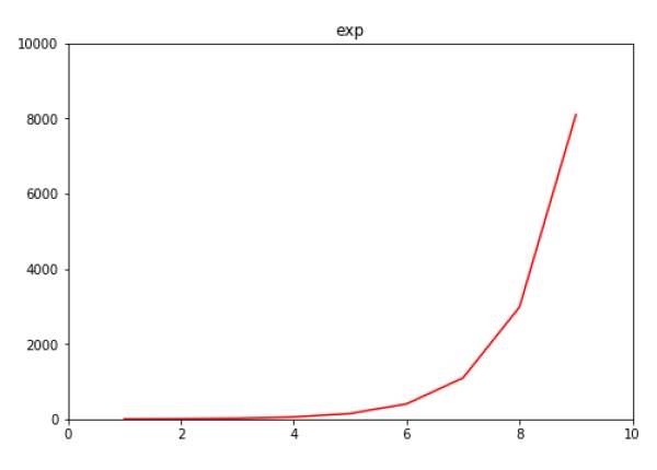
Matplotlib — Setting Ticks and Tick Labels
Ticks are the markers denoting data points on axes. Matplotlib has so far — in all our previous examples — automatically taken over the task of spacing points on the axis.Matplotlib’s default tick locators and formatters are designed to be generally sufficient in many common situations. Position and labels of ticks can be explicitly mentioned to suit specific requirements.
The xticks() and yticks() function takes a list object as argument. The elements in the list denote the positions on corresponding action where ticks will be displayed.
ax.set_xticks([2,4,6,8,10])
This method will mark the data points at the given positions with ticks.
Similarly, labels corresponding to tick marks can be set by set_xlabels() and set_ylabels() functions respectively.
ax.set_xlabels([‘two’, ‘four’,’six’, ‘eight’, ‘ten’])
This will display the text labels below the markers on the x axis.
Following example demonstrates the use of ticks and labels.
import matplotlib.pyplot as plt
import numpy as np
import math
x = np.arange(0, math.pi*2, 0.05)
fig = plt.figure()
ax = fig.add_axes([0.1, 0.1, 0.8, 0.8]) # main axes
y = np.sin(x)
ax.plot(x, y)
ax.set_xlabel(‘angle’)
ax.set_title('sine')
ax.set_xticks([0,2,4,6])
ax.set_xticklabels(['zero','two','four','six'])
ax.set_yticks([-1,0,1])
plt.show()
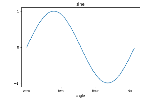
Matplotlib — Twin Axes
It is considered useful to have dual x or y axes in a figure. Moreso, when plotting curves with different units together. Matplotlib supports this with the twinxand twiny functions.
In the following example, the plot has dual y axes, one showing exp(x) and the other showing log(x) −
import matplotlib.pyplot as plt
import numpy as np
fig = plt.figure()
a1 = fig.add_axes([0,0,1,1])
x = np.arange(1,11)
a1.plot(x,np.exp(x))
a1.set_ylabel('exp')
a2 = a1.twinx()
a2.plot(x, np.log(x),'ro-')
a2.set_ylabel('log')
fig.legend(labels = ('exp','log'),loc='upper left')
plt.show()
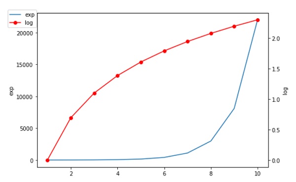
Matplotlib — Bar Plot
A bar chart or bar graph is a chart or graph that presents categorical data with rectangular bars with heights or lengths proportional to the values that they represent. The bars can be plotted vertically or horizontally.
A bar graph shows comparisons among discrete categories. One axis of the chart shows the specific categories being compared, and the other axis represents a measured value.
Matplotlib API provides the bar() function that can be used in the MATLAB style use as well as object oriented API. The signature of bar() function to be used with axes object is as follows −
ax.bar(x, height, width, bottom, align)
The function makes a bar plot with the bound rectangle of size (x −width = 2; x + width=2; bottom; bottom + height).
The parameters to the function are −
| x | sequence of scalars representing the x coordinates of the bars. align controls if x is the bar center (default) or left edge. |
| height | scalar or sequence of scalars representing the height(s) of the bars. |
| width | scalar or array-like, optional. the width(s) of the bars default 0.8 |
| bottom | scalar or array-like, optional. the y coordinate(s) of the bars default None. |
| align | {‘center’, ‘edge’}, optional, default ‘center’ |
The function returns a Matplotlib container object with all bars.
Following is a simple example of the Matplotlib bar plot. It shows the number of students enrolled for various courses offered at an institute.
import matplotlib.pyplot as plt
fig = plt.figure()
ax = fig.add_axes([0,0,1,1])
langs = ['C', 'C++', 'Java', 'Python', 'PHP']
students = [23,17,35,29,12]
ax.bar(langs,students)
plt.show()
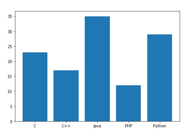
When comparing several quantities and when changing one variable, we might want a bar chart where we have bars of one color for one quantity value.
We can plot multiple bar charts by playing with the thickness and the positions of the bars. The data variable contains three series of four values. The following script will show three bar charts of four bars. The bars will have a thickness of 0.25 units. Each bar chart will be shifted 0.25 units from the previous one. The data object is a multidict containing number of students passed in three branches of an engineering college over the last four years.
import numpy as np
import matplotlib.pyplot as plt
data = [[30, 25, 50, 20],
[40, 23, 51, 17],
[35, 22, 45, 19]]
X = np.arange(4)
fig = plt.figure()
ax = fig.add_axes([0,0,1,1])
ax.bar(X + 0.00, data[0], color = 'b', width = 0.25)
ax.bar(X + 0.25, data[1], color = 'g', width = 0.25)
ax.bar(X + 0.50, data[2], color = 'r', width = 0.25)
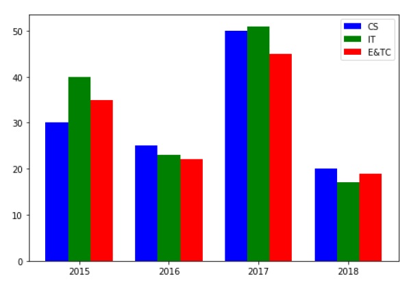
The stacked bar chart stacks bars that represent different groups on top of each other. The height of the resulting bar shows the combined result of the groups.
The optional bottom parameter of the pyplot.bar() function allows you to specify a starting value for a bar. Instead of running from zero to a value, it will go from the bottom to the value. The first call to pyplot.bar() plots the blue bars. The second call to pyplot.bar() plots the red bars, with the bottom of the blue bars being at the top of the red bars.
import numpy as np
import matplotlib.pyplot as plt
N = 5
menMeans = (20, 35, 30, 35, 27)
womenMeans = (25, 32, 34, 20, 25)
ind = np.arange(N) # the x locations for the groups
width = 0.35
fig = plt.figure()
ax = fig.add_axes([0,0,1,1])
ax.bar(ind, menMeans, width, color='r')
ax.bar(ind, womenMeans, width,bottom=menMeans, color='b')
ax.set_ylabel('Scores')
ax.set_title('Scores by group and gender')
ax.set_xticks(ind, ('G1', 'G2', 'G3', 'G4', 'G5'))
ax.set_yticks(np.arange(0, 81, 10))
ax.legend(labels=['Men', 'Women'])
plt.show()
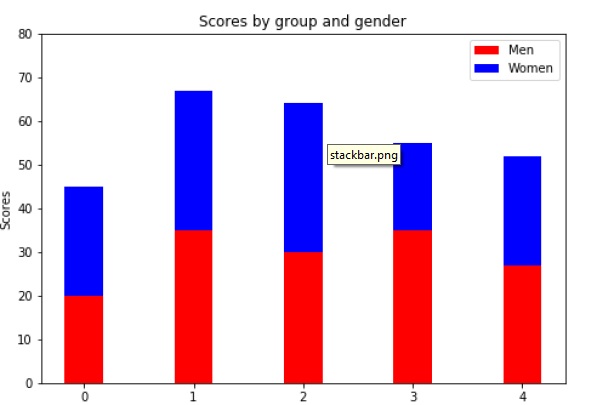
Matplotlib — Histogram
A histogram is an accurate representation of the distribution of numerical data. It is an estimate of the probability distribution of a continuous variable. It is a kind of bar graph.
To construct a histogram, follow these steps −
- Bin the range of values.
- Divide the entire range of values into a series of intervals.
- Count how many values fall into each interval.
The bins are usually specified as consecutive, non-overlapping intervals of a variable.
The matplotlib.pyplot.hist() function plots a histogram. It computes and draws the histogram of x.
Parameters
The following table lists down the parameters for a histogram −
| x | array or sequence of arrays |
| bins | integer or sequence or ‘auto’, optional |
| optional parameters | |
| range | The lower and upper range of the bins. |
| density | If True, the first element of the return tuple will be the counts normalized to form a probability density |
| cumulative | If True, then a histogram is computed where each bin gives the counts in that bin plus all bins for smaller values. |
| histtype | The type of histogram to draw. Default is ‘bar’
|
Following example plots a histogram of marks obtained by students in a class. Four bins, 0-25, 26-50, 51-75, and 76-100 are defined. The Histogram shows number of students falling in this range.
from matplotlib import pyplot as plt
import numpy as np
fig,ax = plt.subplots(1,1)
a = np.array([22,87,5,43,56,73,55,54,11,20,51,5,79,31,27])
ax.hist(a, bins = [0,25,50,75,100])
ax.set_title("histogram of result")
ax.set_xticks([0,25,50,75,100])
ax.set_xlabel('marks')
ax.set_ylabel('no. of students')
plt.show()
The plot appears as shown below −
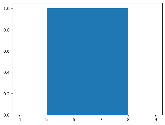
Matplotlib — Pie Chart
A Pie Chart can only display one series of data. Pie charts show the size of items (called wedge) in one data series, proportional to the sum of the items. The data points in a pie chart are shown as a percentage of the whole pie.
Matplotlib API has a pie() function that generates a pie diagram representing data in an array. The fractional area of each wedge is given by x/sum(x). If sum(x)< 1, then the values of x give the fractional area directly and the array will not be normalized. Theresulting pie will have an empty wedge of size 1 — sum(x).
The pie chart looks best if the figure and axes are square, or the Axes aspect is equal.
Parameters
Following table lists down the parameters foe a pie chart −
| x | array-like. The wedge sizes. |
| labels | list. A sequence of strings providing the labels for each wedge. |
| Colors | A sequence of matplotlibcolorargs through which the pie chart will cycle. If None, will use the colors in the currently active cycle. |
| Autopct | string, used to label the wedges with their numeric value. The label will be placed inside the wedge. The format string will be fmt%pct. |
Following code uses the pie() function to display the pie chart of the list of students enrolled for various computer language courses. The proportionate percentage is displayed inside the respective wedge with the help of autopct parameter which is set to %1.2f%.
from matplotlib import pyplot as plt
import numpy as np
fig = plt.figure()
ax = fig.add_axes([0,0,1,1])
ax.axis('equal')
langs = ['C', 'C++', 'Java', 'Python', 'PHP']
students = [23,17,35,29,12]
ax.pie(students, labels = langs,autopct='%1.2f%%')
plt.show()

Matplotlib — Scatter Plot
Scatter plots are used to plot data points on horizontal and vertical axis in the attempt to show how much one variable is affected by another. Each row in the data table is represented by a marker the position depends on its values in the columns set on the X and Y axes. A third variable can be set to correspond to the color or size of the markers, thus adding yet another dimension to the plot.
The script below plots a scatter diagram of grades range vs grades of boys and girls in two different colors.
import matplotlib.pyplot as plt
girls_grades = [89, 90, 70, 89, 100, 80, 90, 100, 80, 34]
boys_grades = [30, 29, 49, 48, 100, 48, 38, 45, 20, 30]
grades_range = [10, 20, 30, 40, 50, 60, 70, 80, 90, 100]
fig=plt.figure()
ax=fig.add_axes([0,0,1,1])
ax.scatter(grades_range, girls_grades, color='r')
ax.scatter(grades_range, boys_grades, color='b')
ax.set_xlabel('Grades Range')
ax.set_ylabel('Grades Scored')
ax.set_title('scatter plot')
plt.show()
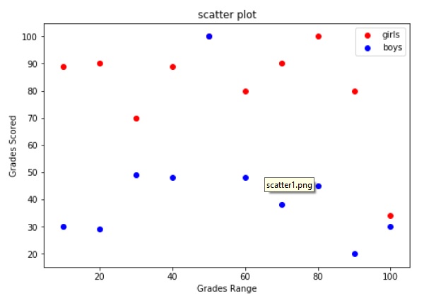
Matplotlib — Contour Plot
Contour plots (sometimes called Level Plots) are a way to show a three-dimensional surface on a two-dimensional plane. It graphs two predictor variables X Y on the y-axis and a response variable Z as contours. These contours are sometimes called the z-slices or the iso-response values.
A contour plot is appropriate if you want to see how alue Z changes as a function of two inputs X and Y, such that Z = f(X,Y). A contour line or isoline of a function of two variables is a curve along which the function has a constant value.
The independent variables x and y are usually restricted to a regular grid called meshgrid. The numpy.meshgrid creates a rectangular grid out of an array of x values and an array of y values.
Matplotlib API contains contour() and contourf() functions that draw contour lines and filled contours, respectively. Both functions need three parameters x,y and z.
import numpy as np
import matplotlib.pyplot as plt
xlist = np.linspace(-3.0, 3.0, 100)
ylist = np.linspace(-3.0, 3.0, 100)
X, Y = np.meshgrid(xlist, ylist)
Z = np.sqrt(X**2 + Y**2)
fig,ax=plt.subplots(1,1)
cp = ax.contourf(X, Y, Z)
fig.colorbar(cp) # Add a colorbar to a plot
ax.set_title('Filled Contours Plot')
#ax.set_xlabel('x (cm)')
ax.set_ylabel('y (cm)')
plt.show()
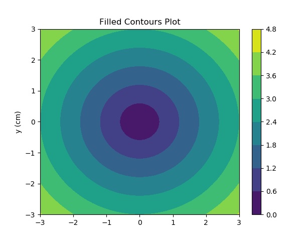
Matplotlib — Quiver Plot
A quiver plot displays the velocity vectors as arrows with components (u,v) at the points (x,y).
quiver(x,y,u,v)
The above command plots vectors as arrows at the coordinates specified in each corresponding pair of elements in x and y.
Parameters
The following table lists down the different parameters for the Quiver plot −
| x | 1D or 2D array, sequence. The x coordinates of the arrow locations |
| y | 1D or 2D array, sequence. The y coordinates of the arrow locations |
| u | 1D or 2D array, sequence. The x components of the arrow vectors |
| v | 1D or 2D array, sequence. The y components of the arrow vectors |
| c | 1D or 2D array, sequence. The arrow colors |
The following code draws a simple quiver plot −
import matplotlib.pyplot as plt
import numpy as np
x,y = np.meshgrid(np.arange(-2, 2, .2), np.arange(-2, 2, .25))
z = x*np.exp(-x**2 - y**2)
v, u = np.gradient(z, .2, .2)
fig, ax = plt.subplots()
q = ax.quiver(x,y,u,v)
plt.show()

Matplotlib — Box Plot
A box plot which is also known as a whisker plot displays a summary of a set of data containing the minimum, first quartile, median, third quartile, and maximum. In a box plot, we draw a box from the first quartile to the third quartile. A vertical line goes through the box at the median. The whiskers go from each quartile to the minimum or maximum.
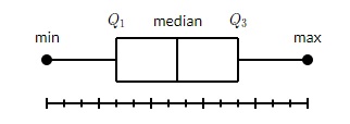
Let us create the data for the boxplots. We use the numpy.random.normal() function to create the fake data. It takes three arguments, mean and standard deviation of the normal distribution, and the number of values desired.
np.random.seed(10)
collectn_1 = np.random.normal(100, 10, 200)
collectn_2 = np.random.normal(80, 30, 200)
collectn_3 = np.random.normal(90, 20, 200)
collectn_4 = np.random.normal(70, 25, 200)
The list of arrays that we created above is the only required input for creating the boxplot. Using the data_to_plot line of code, we can create the boxplot with the following code −
fig = plt.figure()
# Create an axes instance
ax = fig.add_axes([0,0,1,1])
# Create the boxplot
bp = ax.boxplot(data_to_plot)
plt.show()
The above line of code will generate the following output −

Matplotlib — Violin Plot
Violin plots are similar to box plots, except that they also show the probability density of the data at different values. These plots include a marker for the median of the data and a box indicating the interquartile range, as in the standard box plots. Overlaid on this box plot is a kernel density estimation. Like box plots, violin plots are used to represent comparison of a variable distribution (or sample distribution) across different «categories».
A violin plot is more informative than a plain box plot. In fact while a box plot only shows summary statistics such as mean/median and interquartile ranges, the violin plot shows the full distribution of the data.
import matplotlib.pyplot as plt
import numpy as np

np.random.seed(10)
collectn_1 = np.random.normal(100, 10, 200)
collectn_2 = np.random.normal(80, 30, 200)
collectn_3 = np.random.normal(90, 20, 200)
collectn_4 = np.random.normal(70, 25, 200)

## combine these different collections into a list
data_to_plot = [collectn_1, collectn_2, collectn_3, collectn_4]

# Create a figure instance
fig = plt.figure()

# Create an axes instance
ax = fig.add_axes([0,0,1,1])

# Create the boxplot
bp = ax.violinplot(data_to_plot)
plt.show()
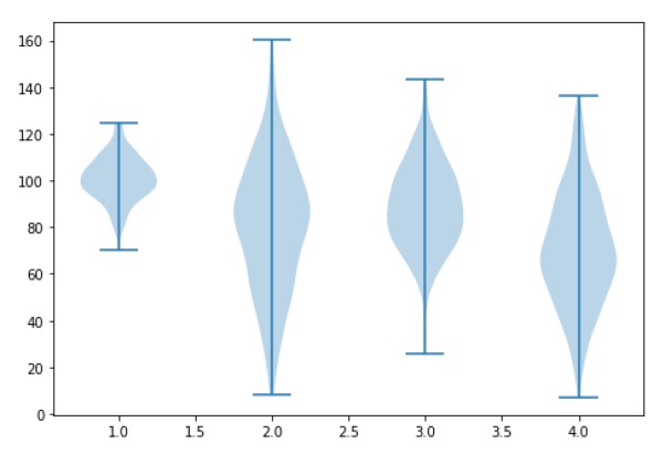
Matplotlib — Three-dimensional Plotting
Even though Matplotlib was initially designed with only two-dimensional plotting in mind, some three-dimensional plotting utilities were built on top of Matplotlib’s two-dimensional display in later versions, to provide a set of tools for three-dimensional data visualization. Three-dimensional plots are enabled by importing the mplot3d toolkit, included with the Matplotlib package.
A three-dimensional axes can be created by passing the keyword projection=’3d’ to any of the normal axes creation routines.
from mpl_toolkits import mplot3d
import numpy as np
import matplotlib.pyplot as plt
fig = plt.figure()
ax = plt.axes(projection='3d')
z = np.linspace(0, 1, 100)
x = z * np.sin(20 * z)
y = z * np.cos(20 * z)
ax.plot3D(x, y, z, 'gray')
ax.set_title('3D line plot')
plt.show()
We can now plot a variety of three-dimensional plot types. The most basic three-dimensional plot is a 3D line plot created from sets of (x, y, z) triples. This can be created using the ax.plot3D function.
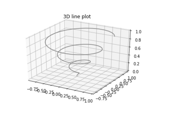
3D scatter plot is generated by using the ax.scatter3D function.
from mpl_toolkits import mplot3d
import numpy as np
import matplotlib.pyplot as plt
fig = plt.figure()
ax = plt.axes(projection='3d')
z = np.linspace(0, 1, 100)
x = z * np.sin(20 * z)
y = z * np.cos(20 * z)
c = x + y
ax.scatter(x, y, z, c=c)
ax.set_title('3d Scatter plot')
plt.show()
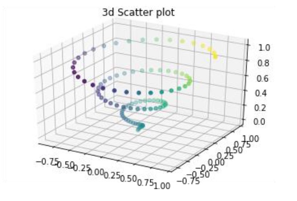
Matplotlib — 3D Contour Plot
The ax.contour3D() function creates three-dimensional contour plot. It requires all the input data to be in the form of two-dimensional regular grids, with the Z-data evaluated at each point. Here, we will show a three-dimensional contour diagram of a three-dimensional sinusoidal function.
from mpl_toolkits import mplot3d
import numpy as np
import matplotlib.pyplot as plt
def f(x, y):
   return np.sin(np.sqrt(x ** 2 + y ** 2))

x = np.linspace(-6, 6, 30)
y = np.linspace(-6, 6, 30)

X, Y = np.meshgrid(x, y)
Z = f(X, Y)

fig = plt.figure()
ax = plt.axes(projection='3d')
ax.contour3D(X, Y, Z, 50, cmap='binary')
ax.set_xlabel('x')
ax.set_ylabel('y')
ax.set_zlabel('z')
ax.set_title('3D contour')
plt.show()

Matplotlib — 3D Wireframe plot
Wireframe plot takes a grid of values and projects it onto the specified three-dimensional surface, and can make the resulting three-dimensional forms quite easy to visualize. The plot_wireframe() function is used for the purpose −
from mpl_toolkits import mplot3d
import numpy as np
import matplotlib.pyplot as plt
def f(x, y):
   return np.sin(np.sqrt(x ** 2 + y ** 2))

x = np.linspace(-6, 6, 30)
y = np.linspace(-6, 6, 30)

X, Y = np.meshgrid(x, y)
Z = f(X, Y)

fig = plt.figure()
ax = plt.axes(projection='3d')
ax.plot_wireframe(X, Y, Z, color='black')
ax.set_title('wireframe')
plt.show()
The above line of code will generate the following output −

Matplotlib — 3D Surface plot
Surface plot shows a functional relationship between a designated dependent variable (Y), and two independent variables (X and Z). The plot is a companion plot to the contour plot. A surface plot is like a wireframe plot, but each face of the wireframe is a filled polygon. This can aid perception of the topology of the surface being visualized. The plot_surface() function x,y and z as arguments.
from mpl_toolkits import mplot3d
import numpy as np
import matplotlib.pyplot as plt
x = np.outer(np.linspace(-2, 2, 30), np.ones(30))
y = x.copy().T # transpose
z = np.cos(x ** 2 + y ** 2)

fig = plt.figure()
ax = plt.axes(projection='3d')

ax.plot_surface(x, y, z,cmap='viridis', edgecolor='none')
ax.set_title('Surface plot')
plt.show()
The above line of code will generate the following output −
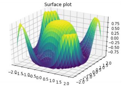
Matplotlib — Working With Text
Matplotlib has extensive text support, including support for mathematical expressions, TrueType support for raster and vector outputs, newline separated text with arbitrary rotations, and unicode support. Matplotlib includes its own matplotlib.font_manager which implements a cross platform, W3C compliant font finding algorithm.
The user has a great deal of control over text properties (font size, font weight, text location and color, etc.). Matplotlib implements a large number of TeX math symbols and commands.
The following list of commands are used to create text in the Pyplot interface −
| text | Add text at an arbitrary location of the Axes. |
| annotate | Add an annotation, with an optional arrow, at an arbitrary location of theAxes. |
| xlabel | Add a label to the Axes’s x-axis. |
| ylabel | Add a label to the Axes’s y-axis. |
| title | Add a title to the Axes. |
| figtext | Add text at an arbitrary location of the Figure. |
| suptitle | Add a title to the Figure. |
All of these functions create and return a matplotlib.text.Text() instance.
Following scripts demonstrate the use of some of the above functions −
import matplotlib.pyplot as plt
fig = plt.figure()

ax = fig.add_axes([0,0,1,1])

ax.set_title('axes title')
ax.set_xlabel('xlabel')
ax.set_ylabel('ylabel')
ax.text(3, 8, 'boxed italics text in data coords', style='italic',
bbox = {'facecolor': 'red'})
ax.text(2, 6, r'an equation: $E = mc^2$', fontsize = 15)
ax.text(4, 0.05, 'colored text in axes coords',
verticalalignment = 'bottom', color = 'green', fontsize = 15)
ax.plot([2], [1], 'o')
ax.annotate('annotate', xy = (2, 1), xytext = (3, 4),
arrowprops = dict(facecolor = 'black', shrink = 0.05))
ax.axis([0, 10, 0, 10])
plt.show()
The above line of code will generate the following output −

Matplotlib — Mathematical Expressions
You can use a subset TeXmarkup in any Matplotlib text string by placing it inside a pair of dollar signs ($).
# math text
plt.title(r'$alpha > beta$')
To make subscripts and superscripts, use the ‘_’ and ‘^’ symbols −
r'$alpha_i> beta_i$'

import numpy as np
import matplotlib.pyplot as plt
t = np.arange(0.0, 2.0, 0.01)
s = np.sin(2*np.pi*t)

plt.plot(t,s)
plt.title(r'$alpha_i> beta_i$', fontsize=20)

plt.text(0.6, 0.6, r'$mathcal{A}mathrm{sin}(2 omega t)$', fontsize = 20)
plt.text(0.1, -0.5, r'$sqrt{2}$', fontsize=10)
plt.xlabel('time (s)')
plt.ylabel('volts (mV)')
plt.show()
The above line of code will generate the following output −

Matplotlib — Working with Images
The image module in Matplotlib package provides functionalities required for loading, rescaling and displaying image.
Loading image data is supported by the Pillow library. Natively, Matplotlib only supports PNG images. The commands shown below fall back on Pillow if the native read fails.
The image used in this example is a PNG file, but keep that Pillow requirement in mind for your own data. The imread() function is used to read image data in an ndarray object of float32 dtype.
import matplotlib.pyplot as plt
import matplotlib.image as mpimg
import numpy as np
img = mpimg.imread('mtplogo.png')
Assuming that following image named as mtplogo.png is present in the current working directory.

Any array containing image data can be saved to a disk file by executing the imsave() function. Here a vertically flipped version of the original png file is saved by giving origin parameter as lower.
plt.imsave("logo.png", img, cmap = 'gray', origin = 'lower')
The new image appears as below if opened in any image viewer.

To draw the image on Matplotlib viewer, execute the imshow() function.
imgplot = plt.imshow(img)
Matplotlib — Transforms
The matplotlib package is built on top of a transformation framework to easily move between coordinate systems. Four coordinate systems can be used. The systems are described in brief in the table given below −
| Coordinate | Transformation Object | Description |
|---|---|---|
| Data | ax.transData |
The user land data coordinate system. controlled by the xlim and ylim |
| Axes | ax.transAxes |
The coordinate system of the Axes. (0,0) is bottom left and (1,1) is top right of the axes. |
| Figure | fig.transFigure |
The coordinate system of the Figure. (0,0) is bottom left and (1,1) is top right of the figure |
| display | None |
This is the pixel coordinate system of the display. (0,0) is the bottom left and (width, height) is the top right of display in pixels. Alternatively, the(matplotlib.transforms.IdentityTransform()) may be used instead of None. |
Consider the following example −
axes.text(x,y,"my label")
The text is placed at the theoretical position of a data point (x,y). Thus we would speak of «data coords».
Using other transformation objects, placement can be controlled. For example, if the above test is to be placed in the centre of axes coordinate system, execute the following line of code −
axes.text(0.5, 0.5, "middle of graph", transform=axes.transAxes)
These transformations can be used for any kind of Matplotlib objects. The default transformation for ax.text is ax.transData and the default transformation for fig.text is fig.transFigure.
The axes coordinate system is extremely useful when placing text in your axes. You might often want a text bubble in a fixed location; for example, on the upper left of the axes pane and have that location remain fixed when you pan or zoom.
Matplotlib – наиболее широко используемый инструмент на Python. Он имеет отличную поддержку множеством сред, таких, как веб-серверы приложений, графические библиотеки пользовательского интерфейса, Jupiter Notebook, iPython Notebook и оболочка iPython.
Примечание редакции
Текст публикуется в переводе, автор оригинальной статьи – Rashida Nasrin Sucky. Примеры кода в оригинале содержали большое количество ошибок, которые нашему автору пришлось исправить в русскоязычной версии публикации.
Matplotlib имеет три основных слоя: слой нижнего уровня (backend), слой рисунков и слой скриптов. Слой нижнего уровня содержит три интерфейсных класса: канва рисунка (figure canvas), определяющая область рисунка, прорисовщик (renderer), умеющий рисовать на этой канве, и событие (event), обрабатывающее ввод пользователя вроде щелчков мыши. Слой рисунков знает, как рисовать с помощью Renderer’а и рисовать на канве. Все, что находится на рисунке Matplotlib, является экземпляром слоя рисунка (artist). Засечки, заголовок, метки – все это индивидуальные объекты слоя рисунков. Слой скриптов – это облегченный интерфейс, который очень полезен для ежедневного применения. Все примеры, приведенные в этой статье, используют слой скриптов и среду Jupiter Notebook.
Если вы используете эту статью для обучения, я рекомендую вам запускать каждый пример кода.
Подготовка данных
Подготовка данных – часто выполняемая задача перед любым проектом по визуализации данных или анализа данных, поскольку данные никогда не приходят в том виде, в котором они нам нужны. Я использую набор данных об иммиграции в Канаду. Сначала импортируем необходимые пакеты и набор данных.
От переводчика
Для импорта файла xlsx нужно установить пакет xlrd, однако новые версии этого пакета перестали читать файлы xlsx по соображениям безопасности. Чтобы прочитать файл, установите старую версию xlrd командой pip install xlrd==1.2.0.
        import numpy as np
import pandas as pd
df = pd.read_excel('https://s3-api.us-geo.objectstorage.softlayer.net/cf-courses-data/CognitiveClass/DV0101EN/labs/Data_Files/Canada.xlsx',
                       sheet_name='Canada by Citizenship',
                       skiprows=range(20),
                       skipfooter=2)
df.head()
Я пропускаю первые 20 строк и последние две строки, потому что это текст, а не данные с табуляцией. Набор данных слишком велик, так что я не могу показать его целиком. Чтобы получить представление о наборе, давайте посмотрим на имена столбцов:
        df.columns
# Вывод:
# Index([    'Type', 'Coverage',   'OdName',     'AREA', 'AreaName',      'REG',
#        'RegName',      'DEV',  'DevName',       1980,       1981,       1982,
#             1983,       1984,       1985,       1986,       1987,       1988,
#             1989,       1990,       1991,       1992,       1993,       1994,
#             1995,       1996,       1997,       1998,       1999,       2000,
#             2001,       2002,       2003,       2004,       2005,       2006,
#             2007,       2008,       2009,       2010,       2011,       2012,
#             2013],
#      dtype='object')
Мы не собираемся использовать все эти столбцы в нашей статье. Поэтому давайте избавимся от столбцов, которые мы не будем использовать, чтобы сделать набор данных меньшим и лучше управляемым.
        df.drop(['AREA','REG','DEV','Type','Coverage'], axis=1, inplace=True)
df.head()
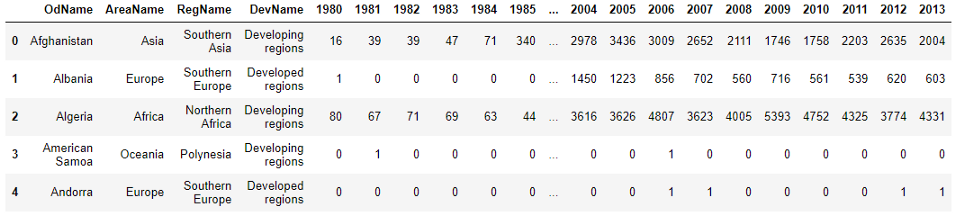
Посмотрите на эти столбцы. Столбец ‘OdName’ – на самом деле название страны, ‘AreaName’ – континент, а ‘RegName’ – регион на этом континенте. Переименуем эти столбцы, чтобы их имена стали более понятными.
        df.rename(columns={'OdName':'Country', 'AreaName':'Continent', 'RegName':'Region'}, inplace=True)
df.columns
# Вывод:
# Index([  'Country', 'Continent',    'Region',   'DevName',        1980,
#              1981,        1982,        1983,        1984,        1985,
#              1986,        1987,        1988,        1989,        1990,
#              1991,        1992,        1993,        1994,        1995,
#              1996,        1997,        1998,        1999,        2000,
#              2001,        2002,        2003,        2004,        2005,
#              2006,        2007,        2008,        2009,        2010,
#              2011,        2012,        2013],
#      dtype='object')
Теперь наш набор данных стал более простым для понимания. У нас есть Country, Continent, Region, а DevName указывает, является ли страна развитой или развивающейся. Все столбцы с годами содержат количество иммигрантов в Канаду из соответствующей страны за указанный год. Теперь добавим столбец ‘Total’ (‘Всего’), в котором будет содержаться общее количество иммигрантов из этой страны с 1980-го до 2013-го.
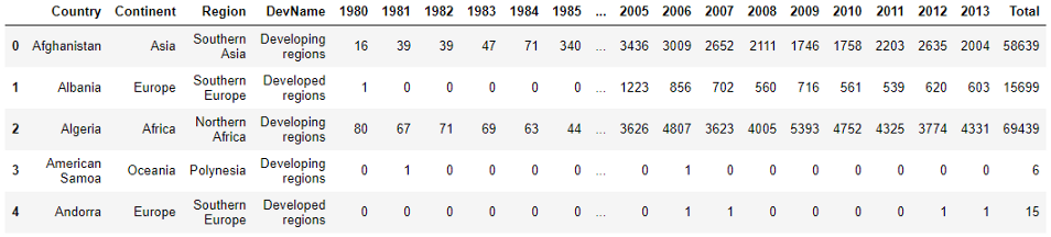
Проверим, есть ли в наборе какие-либо значения null.
df.isnull().sum()
Результат показывает 0 во всех столбцах, то есть в наборе нет пропусков. Я люблю задавать в качестве индекса значащий столбец, а не какие-то цифры, поэтому установим столбец ‘Country’ в качестве индекса.
df = df.set_index('Country')
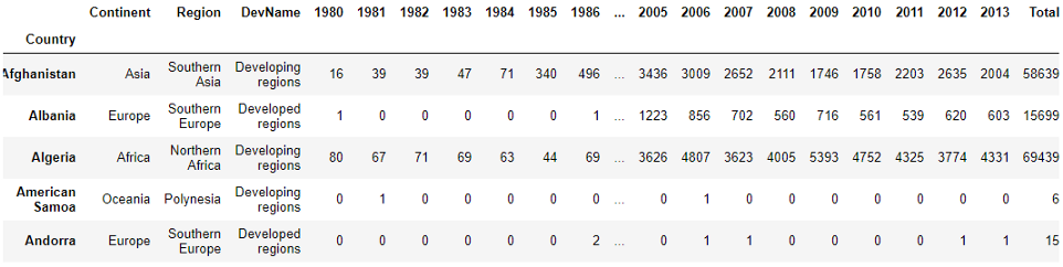
Теперь набор данных достаточно чист и красив, чтобы начать работать с ним, поэтому больше чистить мы не станем. Если нам потребуется что-то еще, мы сделаем это по мере необходимости.
Упражнения по рисованию диаграмм
В этой статье мы попробуем несколько различных типов диаграмм – таких, как линейная диаграмма (line plot), диаграмма с областями (area plot), секторная диаграмма (pie plot), диаграмма рассеяния (scatter plot), гистограмма, столбчатая диаграмма (bar graph). Сначала импортируем необходимые пакеты.
        %matplotlib inline
import matplotlib.pyplot as plt
import matplotlib as mpl
Выберем стиль, чтобы нам не пришлось слишком утруждаться установкой стиля диаграммы. Вот список доступных стилей:
        plt.style.available
# Вывод:
# ['bmh',
#  'classic',
#  'dark_background',
#  'fast',
#  'fivethirtyeight',
#  'ggplot',
#  'grayscale',
#  'seaborn-bright',
#  'seaborn-colorblind',
#  'seaborn-dark-palette',
#  'seaborn-dark',
#  'seaborn-darkgrid',
#  'seaborn-deep',
#  'seaborn-muted',
#  'seaborn-notebook',
#  'seaborn-paper',
#  'seaborn-pastel',
#  'seaborn-poster',
#  'seaborn-talk',
#  'seaborn-ticks',
#  'seaborn-white',
#  'seaborn-whitegrid',
#  'seaborn',
#  'Solarize_Light2',
#  'tableau-colorblind10',
#  '_classic_test']
Я буду использовать стиль ‘ggplot’. Вы можете взять любой другой стиль по своему вкусу.
mpl.style.use(['ggplot'])
Линейная диаграмма
Будет полезным увидеть график изменений иммиграции в Канаду для одной страны. Создадим список лет с 1980-го до 2013-го:
years = list(range(1980, 2014))
Я выбрала для этой демонстрации Швейцарию. Приготовим иммиграционные данные по нашим годам для этой страны.
df.loc['Switzerland', years]
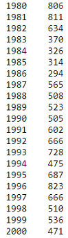
Настало время нарисовать диаграмму. Это очень просто: достаточно вызвать функцию plot для приготовленных нами данных. Затем добавим заголовок и метки для осей x и y.
        df.loc['Switzerland', years].plot()
plt.title('Immigration from Switzerland')
plt.ylabel('Number of immigrants')
plt.xlabel('Years')
plt.show()
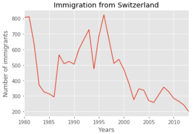
Что, если мы хотим вывести графики иммиграции для нескольких стран сразу, чтобы сравнить тенденции иммиграции из этих стран в Канаду? Это делается почти так же, как и в прошлом примере. Нарисуем диаграмму иммиграции из трех южно-азиатских стран: Индии, Пакистана и Бангладеш по годам.
        ind_pak_ban = df.loc[['India', 'Pakistan', 'Bangladesh'], years]
ind_pak_ban.head()
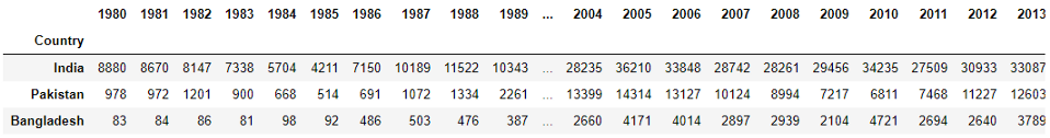
Посмотрите на формат этих данных – он отличается от данных по Швейцарии, использованных прежде. Если мы вызовем функцию plot для этого DataFrame (ind_pak_ban), она выведет количество иммигрантов в каждой стране по оси x и годы по оси y. Нам нужно изменить формат данных:
ind_pak_ban.T
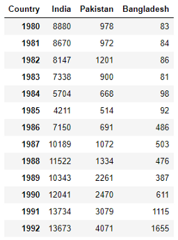
Это не весь набор данных, а только его часть. Видите, теперь формат данных изменился. Теперь годы будут выводиться по оси x, а количество иммигрантов из каждой страны по оси y.
ind_pak_ban.T.plot()
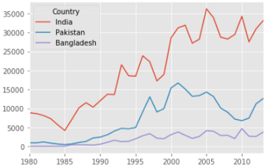
Нам не пришлось задавать тип диаграммы, потому что линейная диаграмма рисуется по умолчанию.
Секторная диаграмма
Чтобы продемонстрировать секторную диаграмму, построим диаграмму общего количества иммигрантов для каждого континента. У нас есть данные по каждой стране. Давайте сгруппируем данные по континентам, чтобы просуммировать количество иммигрантов для каждого континента.
cont = df.groupby('Continent', axis=0).sum()
Теперь у нас есть данные, показывающие общее количество иммигрантов для каждого континента. Если хотите, можете вывести этот DataFrame, чтобы увидеть результат. Я не привожу его потому, что он занимает слишком много места по горизонтали. Давайте нарисуем эту диаграмму.
        cont['Total'].plot(kind='pie', figsize=(7,7),
                  autopct='%1.1f%%',
                  shadow=True)
# plt.title('Immigration By Continenets')
plt.axis('equal')
plt.show()
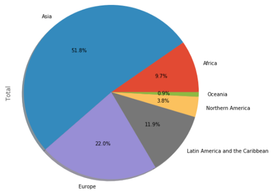
Заметьте, что мне пришлось использовать параметр ‘kind’. Все виды диаграмм, кроме линейной, в функции plot нужно указывать явно. Я ввожу новый параметр ‘figsize’, определяющий размеры диаграммы.
Эта секторная диаграмма достаточно понятна, но мы можем сделать ее еще лучшей. На этот раз я установлю собственные цвета и начальный угол.
        colors = ['lightgreen', 'lightblue', 'pink', 'purple', 'grey', 'gold']
explode=[0.1, 0, 0, 0, 0.1, 0.1]
cont['Total'].plot(kind='pie', figsize=(17, 10),
                  autopct = '%1.1f%%', startangle=90,
                  shadow=True, labels=None, pctdistance=1.12, colors=colors, explode = explode)
plt.axis('equal')
plt.legend(labels=cont.index, loc='upper right', fontsize=14)
plt.show()
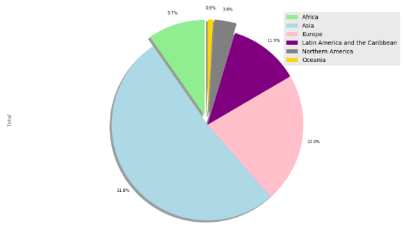
Ящик с усами (boxplot)
Сначала мы построим «ящик с усами» для количества иммигрантов из Китая.
china = df.loc[['China'], years].T
Вот наши данные. А вот диаграмма, построенная по этим данным.
        china.plot(kind='box', figsize=(8, 6))
plt.title('Box plot of Chinese Immigrants')
plt.ylabel('Number of Immigrants')
plt.show()
Если вам нужно освежить свои знания про «ящики с усами», пожалуйста, обратитесь к статье «Пример понимания данных с помощью гистограммы и ящика с усами».
Мы можем нарисовать несколько ящиков с усами в одной диаграмме. Используем DataFrame ind_pak_ban и нарисуем ящики для количества иммигрантов из Индии, Пакистана и Бангладеш.
        ind_pak_ban.T.plot(kind='box', figsize=(8, 7))
plt.title('Box plots of Inian, Pakistan and Bangladesh Immigrants')
plt.ylabel('Number of Immigrants')
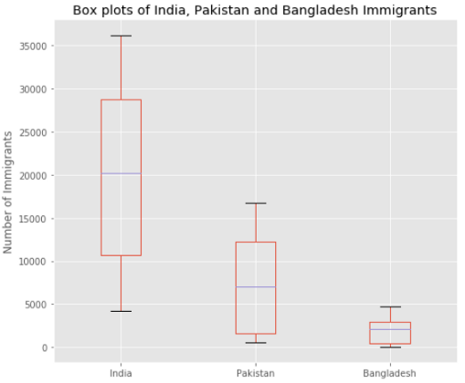
Диаграмма рассеяния
Диаграммы рассеяния лучше всего подходят для исследования зависимости между переменными. Построим диаграмму рассеяния, чтобы увидеть тренд количества иммигрантов в Канаду за годы.
Для этого упражнения мы создадим новый DataFrame, содержащий годы в качестве индекса и общее количество иммигрантов за каждый год.
        totalPerYear = pd.DataFrame(df[years].sum(axis=0))
totalPerYear.head()
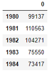
Нам нужно преобразовать годы в целые числа. Я также хочу немного причесать DataFrame, чтобы сделать его более презентабельным.
        totalPerYear.index = map(int, totalPerYear.index)
totalPerYear.reset_index(inplace=True)
totalPerYear.columns = ['year', 'total']
totalPerYear.head()
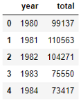
Осталось задать параметры осей x и y для диаграммы рассеяния.
        totalPerYear.plot(kind='scatter', x = 'year', y='total', figsize=(10, 6), color='darkred')
plt.title('Total Immigration from 1980 - 2013')
plt.xlabel('Year')
plt.ylabel('Number of Immigrants')
plt.show()
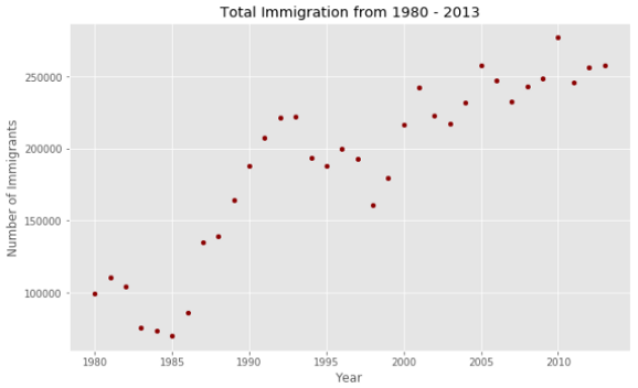
Похоже, здесь есть линейная зависимость между годом и количеством иммигрантов. С течением лет количество иммигрантов показывает явно растущий тренд.
Диаграмма с областями
Диаграмма с областями показывает область под линейным графиком. Для этой диаграммы я хочу создать DataFrame, содержащий информацию по Индии, Китаю, Пакистану и Франции.
        top = df.loc[['India', 'China', 'Pakistan', 'France'], years]
top = top.T
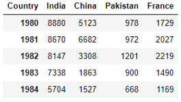
Набор данных готов. Пора сделать из него диаграмму.
        colors = ['black', 'green', 'blue', 'red']
top.plot(kind='area', stacked=False, figsize=(20, 10), color=colors)
plt.title('Immigration trend from Europe')
plt.ylabel('Number of Immigrants')
plt.xlabel('Years')
plt.show()
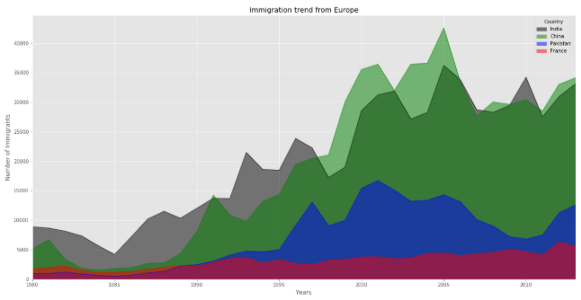
Не забудьте использовать параметр ‘stacked’, если хотите увидеть области для каждой отдельной страны. Если не установить stacked = False, диаграмма будет выглядеть примерно так:
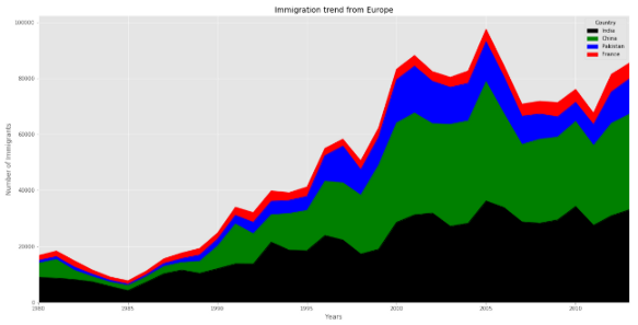
Гистограмма
Гистограмма показывает распределение переменной. Вот ее пример:
        df[2005].plot(kind='hist', figsize=(8,5))
plt.title('Histogram of Immigration from 195 Countries in 2005') # заголовок гистограммы
plt.ylabel('Number of Countries') # y-метка
plt.xlabel('Number of Immigrants') # x-метка
plt.show()
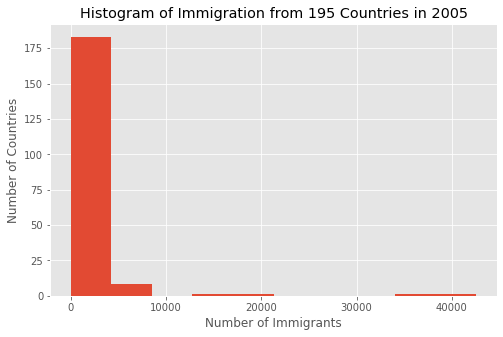
Мы построили гистограмму, показывающую распределение иммиграции за 2005 год. Гистограмма показывает, что из большинства стран приехало от 0 до 5000 иммигрантов. Только несколько стран прислали 20 тысяч, и еще пара стран прислала по 40 тысяч иммигрантов.
Давайте используем DataFrame top из предыдущего примера и нарисуем распределение количества иммигрантов из каждой страны в одной и той же гистограмме.
        top.plot.hist()
plt.title('Histogram of Immigration from Some Populous Countries')
plt.ylabel('Number of Years')
plt.xlabel('Number of Immigrants')
plt.show()
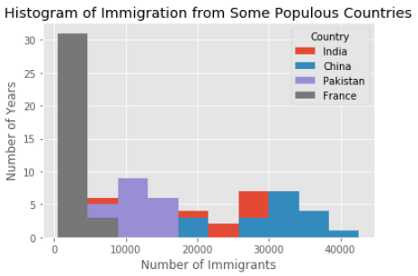
На предыдущей гистограмме мы видели, что из нескольких стран приехало 20 и 40 тысяч иммигрантов. Похоже, что Китай и Индия среди этих «нескольких». На этой гистограмме мы не можем четко увидеть границы между столбцами. Давайте улучшим ее.
Задаем количество столбцов и показываем их границы.
Я использую 15 столбцов. Здесь я ввожу новый параметр под названием ‘alpha’ – он определяет прозрачность цветов. Для таких перекрывающихся диаграмм, как наша, прозрачность важна, чтобы увидеть картину каждого распределения.
        count, bin_edges = np.histogram(top, 15)
top.plot(kind = 'hist', figsize=(14, 6), bins=15, alpha=0.6,
        xticks=bin_edges, color=colors)
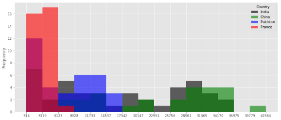
Как и для диаграммы с областями, мы можем использовать параметр ‘stacked’, но для гистограмм он по умолчанию выключен.
        top.plot(kind='hist',
          figsize=(12, 6),
          bins=15,
          xticks=bin_edges,
          color=colors,
          stacked=True,
         )
plt.title('Histogram of Immigration from Some Populous Countries')
plt.ylabel('Number of Years')
plt.xlabel('Number of Immigrants')
plt.show()
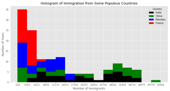
Столбчатая диаграмма
Для столбчатой диаграммы я использую количество иммигрантов из Франции за каждый год.
        france = df.loc['France', years]
france.plot(kind='bar', figsize = (10, 6))
plt.xlabel('Year')
plt.ylabel('Number of immigrants')
plt.title('Immigrants From France')
plt.show()
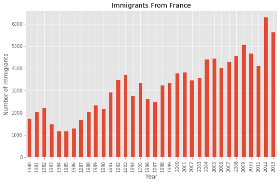
Вы можете добавить к столбчатой диаграмме дополнительную информацию. Эта диаграмма показывает растущий тренд с 1997 года примерно на декаду, который стоит отметить. Это можно сделать с помощью функции annotate.
        france.plot(kind='bar', figsize = (10, 6))
plt.xlabel('Year')
plt.ylabel('Number of immigrants')
plt.title('Immigrants From France')
plt.annotate('Increasing Trend',
            xy = (19, 4500),
            rotation= 23,
            va = 'bottom',
            ha = 'left')
plt.annotate('',
            xy=(29, 5500),
            xytext=(17, 3800),
            xycoords='data',
            arrowprops=dict(arrowstyle='->', connectionstyle='arc3', color='black', lw=1.5))
plt.show()
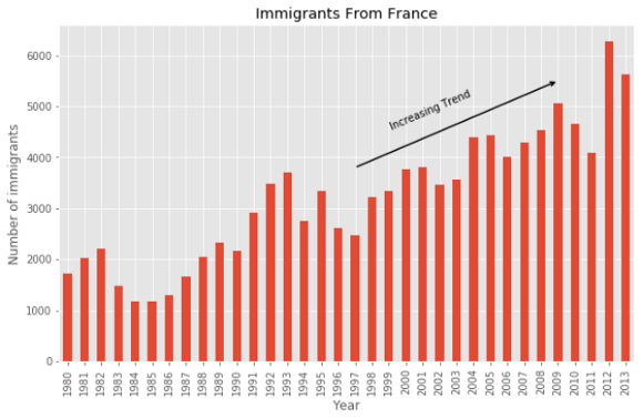
Иногда горизонтальное расположение столбцов делает диаграмму более понятной. Еще лучше, если метки рисуются прямо на столбцах. Давайте сделаем это.
        france.plot(kind='barh', figsize=(12, 16), color='steelblue')
plt.xlabel('Year') # add to x-label to the plot
plt.ylabel('Number of immigrants') # add y-label to the plot
plt.title('Immigrants From France') # add title to the plot
for index, value in enumerate(france):
    label = format(int(value), ',')
    plt.annotate(label, xy=(value-300, index-0.1), color='white')

plt.show()
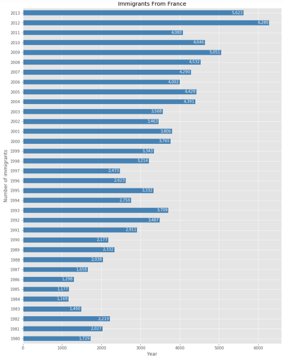
Разве эта диаграмма выглядит не лучше, чем предыдущая?
В этой статье мы изучили основы Matplotlib. Теперь у вас достаточно знаний, чтобы начать самостоятельное использование Matplotlib прямо сегодня.
Расширенные методы визуализации описаны в следующих статьях:
- «Интерактивная фоновая картограмма на Python»
- «Создаем «облака слов» любой формы на Python»
- «Интерактивная визуализация географических данных на Python»
- «Вафельные графики» с помощью Matplotlib на Python»
- «Пузырьковые диаграммы с помощью Matplotlib»
- «Исследовательский анализ данных для моделирования данных»
- «Сортируем и сегментируем данные с помощью методов Cut или Qcut из Pandas»