Prerequisites#
You’ll need to know a bit of Python. For a refresher, see the Python
tutorial.
To work the examples, you’ll need matplotlib installed
in addition to NumPy.
Learner profile
This is a quick overview of arrays in NumPy. It demonstrates how n-dimensional
((n>=2)) arrays are represented and can be manipulated. In particular, if
you don’t know how to apply common functions to n-dimensional arrays (without
using for-loops), or if you want to understand axis and shape properties for
n-dimensional arrays, this article might be of help.
Learning Objectives
After reading, you should be able to:
-
Understand the difference between one-, two- and n-dimensional arrays in
NumPy; -
Understand how to apply some linear algebra operations to n-dimensional
arrays without using for-loops; -
Understand axis and shape properties for n-dimensional arrays.
The Basics#
NumPy’s main object is the homogeneous multidimensional array. It is a
table of elements (usually numbers), all of the same type, indexed by a
tuple of non-negative integers. In NumPy dimensions are called axes.
For example, the array for the coordinates of a point in 3D space,
[1, 2, 1], has one axis. That axis has 3 elements in it, so we say
it has a length of 3. In the example pictured below, the array has 2
axes. The first axis has a length of 2, the second axis has a length of
3.
[[1., 0., 0.],
 [0., 1., 2.]]
NumPy’s array class is called ndarray. It is also known by the alias
array. Note that numpy.array is not the same as the Standard
Python Library class array.array, which only handles one-dimensional
arrays and offers less functionality. The more important attributes of
an ndarray object are:
- ndarray.ndim
-
the number of axes (dimensions) of the array.
- ndarray.shape
-
the dimensions of the array. This is a tuple of integers indicating
the size of the array in each dimension. For a matrix with n rows
and m columns,shapewill be(n,m). The length of the
shapetuple is therefore the number of axes,ndim. - ndarray.size
-
the total number of elements of the array. This is equal to the
product of the elements ofshape. - ndarray.dtype
-
an object describing the type of the elements in the array. One can
create or specify dtype’s using standard Python types. Additionally
NumPy provides types of its own. numpy.int32, numpy.int16, and
numpy.float64 are some examples. - ndarray.itemsize
-
the size in bytes of each element of the array. For example, an
array of elements of typefloat64hasitemsize8 (=64/8),
while one of typecomplex32hasitemsize4 (=32/8). It is
equivalent tondarray.dtype.itemsize. - ndarray.data
-
the buffer containing the actual elements of the array. Normally, we
won’t need to use this attribute because we will access the elements
in an array using indexing facilities.
An example#
>>> import numpy as np
>>> a = np.arange(15).reshape(3, 5)
>>> a
array([[ 0,  1,  2,  3,  4],
       [ 5,  6,  7,  8,  9],
       [10, 11, 12, 13, 14]])
>>> a.shape
(3, 5)
>>> a.ndim
2
>>> a.dtype.name
'int64'
>>> a.itemsize
8
>>> a.size
15
>>> type(a)
<class 'numpy.ndarray'>
>>> b = np.array([6, 7, 8])
>>> b
array([6, 7, 8])
>>> type(b)
<class 'numpy.ndarray'>
Array Creation#
There are several ways to create arrays.
For example, you can create an array from a regular Python list or tuple
using the array function. The type of the resulting array is deduced
from the type of the elements in the sequences.
>>> import numpy as np
>>> a = np.array([2, 3, 4])
>>> a
array([2, 3, 4])
>>> a.dtype
dtype('int64')
>>> b = np.array([1.2, 3.5, 5.1])
>>> b.dtype
dtype('float64')
A frequent error consists in calling array with multiple arguments,
rather than providing a single sequence as an argument.
>>> a = np.array(1, 2, 3, 4)    # WRONG
Traceback (most recent call last):
  ...
TypeError: array() takes from 1 to 2 positional arguments but 4 were given
>>> a = np.array([1, 2, 3, 4])  # RIGHT
array transforms sequences of sequences into two-dimensional arrays,
sequences of sequences of sequences into three-dimensional arrays, and
so on.
>>> b = np.array([(1.5, 2, 3), (4, 5, 6)])
>>> b
array([[1.5, 2. , 3. ],
       [4. , 5. , 6. ]])
The type of the array can also be explicitly specified at creation time:
>>> c = np.array([[1, 2], [3, 4]], dtype=complex)
>>> c
array([[1.+0.j, 2.+0.j],
       [3.+0.j, 4.+0.j]])
Often, the elements of an array are originally unknown, but its size is
known. Hence, NumPy offers several functions to create
arrays with initial placeholder content. These minimize the necessity of
growing arrays, an expensive operation.
The function zeros creates an array full of zeros, the function
ones creates an array full of ones, and the function empty
creates an array whose initial content is random and depends on the
state of the memory. By default, the dtype of the created array is
float64, but it can be specified via the key word argument dtype.
>>> np.zeros((3, 4))
array([[0., 0., 0., 0.],
       [0., 0., 0., 0.],
       [0., 0., 0., 0.]])
>>> np.ones((2, 3, 4), dtype=np.int16)
array([[[1, 1, 1, 1],
        [1, 1, 1, 1],
        [1, 1, 1, 1]],

       [[1, 1, 1, 1],
        [1, 1, 1, 1],
        [1, 1, 1, 1]]], dtype=int16)
>>> np.empty((2, 3))
array([[3.73603959e-262, 6.02658058e-154, 6.55490914e-260],  # may vary
       [5.30498948e-313, 3.14673309e-307, 1.00000000e+000]])
To create sequences of numbers, NumPy provides the arange function
which is analogous to the Python built-in range, but returns an
array.
>>> np.arange(10, 30, 5)
array([10, 15, 20, 25])
>>> np.arange(0, 2, 0.3)  # it accepts float arguments
array([0. , 0.3, 0.6, 0.9, 1.2, 1.5, 1.8])
When arange is used with floating point arguments, it is generally
not possible to predict the number of elements obtained, due to the
finite floating point precision. For this reason, it is usually better
to use the function linspace that receives as an argument the number
of elements that we want, instead of the step:
>>> from numpy import pi
>>> np.linspace(0, 2, 9)                   # 9 numbers from 0 to 2
array([0.  , 0.25, 0.5 , 0.75, 1.  , 1.25, 1.5 , 1.75, 2.  ])
>>> x = np.linspace(0, 2 * pi, 100)        # useful to evaluate function at lots of points
>>> f = np.sin(x)
See also
array,
zeros,
zeros_like,
ones,
ones_like,
empty,
empty_like,
arange,
linspace,
numpy.random.Generator.rand,
numpy.random.Generator.randn,
fromfunction,
fromfile
Printing Arrays#
When you print an array, NumPy displays it in a similar way to nested
lists, but with the following layout:
-
the last axis is printed from left to right,
-
the second-to-last is printed from top to bottom,
-
the rest are also printed from top to bottom, with each slice
separated from the next by an empty line.
One-dimensional arrays are then printed as rows, bidimensionals as
matrices and tridimensionals as lists of matrices.
>>> a = np.arange(6)                    # 1d array
>>> print(a)
[0 1 2 3 4 5]
>>>
>>> b = np.arange(12).reshape(4, 3)     # 2d array
>>> print(b)
[[ 0  1  2]
 [ 3  4  5]
 [ 6  7  8]
 [ 9 10 11]]
>>>
>>> c = np.arange(24).reshape(2, 3, 4)  # 3d array
>>> print(c)
[[[ 0  1  2  3]
  [ 4  5  6  7]
  [ 8  9 10 11]]

 [[12 13 14 15]
  [16 17 18 19]
  [20 21 22 23]]]
See below to get
more details on reshape.
If an array is too large to be printed, NumPy automatically skips the
central part of the array and only prints the corners:
>>> print(np.arange(10000))
[   0    1    2 ... 9997 9998 9999]
>>>
>>> print(np.arange(10000).reshape(100, 100))
[[   0    1    2 ...   97   98   99]
 [ 100  101  102 ...  197  198  199]
 [ 200  201  202 ...  297  298  299]
 ...
 [9700 9701 9702 ... 9797 9798 9799]
 [9800 9801 9802 ... 9897 9898 9899]
 [9900 9901 9902 ... 9997 9998 9999]]
To disable this behaviour and force NumPy to print the entire array, you
can change the printing options using set_printoptions.
>>> np.set_printoptions(threshold=sys.maxsize) # sys module should be imported
Basic Operations#
Arithmetic operators on arrays apply elementwise. A new array is
created and filled with the result.
>>> a = np.array([20, 30, 40, 50])
>>> b = np.arange(4)
>>> b
array([0, 1, 2, 3])
>>> c = a - b
>>> c
array([20, 29, 38, 47])
>>> b**2
array([0, 1, 4, 9])
>>> 10 * np.sin(a)
array([ 9.12945251, -9.88031624,  7.4511316 , -2.62374854])
>>> a < 35
array([ True,  True, False, False])
Unlike in many matrix languages, the product operator * operates
elementwise in NumPy arrays. The matrix product can be performed using
the @ operator (in python >=3.5) or the dot function or method:
>>> A = np.array([[1, 1],
...               [0, 1]])
>>> B = np.array([[2, 0],
...               [3, 4]])
>>> A * B     # elementwise product
array([[2, 0],
       [0, 4]])
>>> A @ B     # matrix product
array([[5, 4],
       [3, 4]])
>>> A.dot(B)  # another matrix product
array([[5, 4],
       [3, 4]])
Some operations, such as += and *=, act in place to modify an
existing array rather than create a new one.
>>> rg = np.random.default_rng(1)  # create instance of default random number generator
>>> a = np.ones((2, 3), dtype=int)
>>> b = rg.random((2, 3))
>>> a *= 3
>>> a
array([[3, 3, 3],
       [3, 3, 3]])
>>> b += a
>>> b
array([[3.51182162, 3.9504637 , 3.14415961],
       [3.94864945, 3.31183145, 3.42332645]])
>>> a += b  # b is not automatically converted to integer type
Traceback (most recent call last):
    ...
numpy.core._exceptions._UFuncOutputCastingError: Cannot cast ufunc 'add' output from dtype('float64') to dtype('int64') with casting rule 'same_kind'
When operating with arrays of different types, the type of the resulting
array corresponds to the more general or precise one (a behavior known
as upcasting).
>>> a = np.ones(3, dtype=np.int32)
>>> b = np.linspace(0, pi, 3)
>>> b.dtype.name
'float64'
>>> c = a + b
>>> c
array([1.        , 2.57079633, 4.14159265])
>>> c.dtype.name
'float64'
>>> d = np.exp(c * 1j)
>>> d
array([ 0.54030231+0.84147098j, -0.84147098+0.54030231j,
       -0.54030231-0.84147098j])
>>> d.dtype.name
'complex128'
Many unary operations, such as computing the sum of all the elements in
the array, are implemented as methods of the ndarray class.
>>> a = rg.random((2, 3))
>>> a
array([[0.82770259, 0.40919914, 0.54959369],
       [0.02755911, 0.75351311, 0.53814331]])
>>> a.sum()
3.1057109529998157
>>> a.min()
0.027559113243068367
>>> a.max()
0.8277025938204418
By default, these operations apply to the array as though it were a list
of numbers, regardless of its shape. However, by specifying the axis
parameter you can apply an operation along the specified axis of an
array:
>>> b = np.arange(12).reshape(3, 4)
>>> b
array([[ 0,  1,  2,  3],
       [ 4,  5,  6,  7],
       [ 8,  9, 10, 11]])
>>>
>>> b.sum(axis=0)     # sum of each column
array([12, 15, 18, 21])
>>>
>>> b.min(axis=1)     # min of each row
array([0, 4, 8])
>>>
>>> b.cumsum(axis=1)  # cumulative sum along each row
array([[ 0,  1,  3,  6],
       [ 4,  9, 15, 22],
       [ 8, 17, 27, 38]])
Universal Functions#
NumPy provides familiar mathematical functions such as sin, cos, and
exp. In NumPy, these are called “universal
functions” (ufunc). Within NumPy, these functions
operate elementwise on an array, producing an array as output.
>>> B = np.arange(3)
>>> B
array([0, 1, 2])
>>> np.exp(B)
array([1.        , 2.71828183, 7.3890561 ])
>>> np.sqrt(B)
array([0.        , 1.        , 1.41421356])
>>> C = np.array([2., -1., 4.])
>>> np.add(B, C)
array([2., 0., 6.])
See also
all,
any,
apply_along_axis,
argmax,
argmin,
argsort,
average,
bincount,
ceil,
clip,
conj,
corrcoef,
cov,
cross,
cumprod,
cumsum,
diff,
dot,
floor,
inner,
invert,
lexsort,
max,
maximum,
mean,
median,
min,
minimum,
nonzero,
outer,
prod,
re,
round,
sort,
std,
sum,
trace,
transpose,
var,
vdot,
vectorize,
where
Indexing, Slicing and Iterating#
One-dimensional arrays can be indexed, sliced and iterated over,
much like
lists
and other Python sequences.
>>> a = np.arange(10)**3
>>> a
array([  0,   1,   8,  27,  64, 125, 216, 343, 512, 729])
>>> a[2]
8
>>> a[2:5]
array([ 8, 27, 64])
>>> # equivalent to a[0:6:2] = 1000;
>>> # from start to position 6, exclusive, set every 2nd element to 1000
>>> a[:6:2] = 1000
>>> a
array([1000,    1, 1000,   27, 1000,  125,  216,  343,  512,  729])
>>> a[::-1]  # reversed a
array([ 729,  512,  343,  216,  125, 1000,   27, 1000,    1, 1000])
>>> for i in a:
...     print(i**(1 / 3.))
...
9.999999999999998
1.0
9.999999999999998
3.0
9.999999999999998
4.999999999999999
5.999999999999999
6.999999999999999
7.999999999999999
8.999999999999998
Multidimensional arrays can have one index per axis. These indices
are given in a tuple separated by commas:
>>> def f(x, y):
...     return 10 * x + y
...
>>> b = np.fromfunction(f, (5, 4), dtype=int)
>>> b
array([[ 0,  1,  2,  3],
       [10, 11, 12, 13],
       [20, 21, 22, 23],
       [30, 31, 32, 33],
       [40, 41, 42, 43]])
>>> b[2, 3]
23
>>> b[0:5, 1]  # each row in the second column of b
array([ 1, 11, 21, 31, 41])
>>> b[:, 1]    # equivalent to the previous example
array([ 1, 11, 21, 31, 41])
>>> b[1:3, :]  # each column in the second and third row of b
array([[10, 11, 12, 13],
       [20, 21, 22, 23]])
When fewer indices are provided than the number of axes, the missing
indices are considered complete slices:
>>> b[-1]   # the last row. Equivalent to b[-1, :]
array([40, 41, 42, 43])
The expression within brackets in b[i] is treated as an i
followed by as many instances of : as needed to represent the
remaining axes. NumPy also allows you to write this using dots as
b[i, ...].
The dots (...) represent as many colons as needed to produce a
complete indexing tuple. For example, if x is an array with 5
axes, then
-
x[1, 2, ...]is equivalent tox[1, 2, :, :, :], -
x[..., 3]tox[:, :, :, :, 3]and -
x[4, ..., 5, :]tox[4, :, :, 5, :].
>>> c = np.array([[[  0,  1,  2],  # a 3D array (two stacked 2D arrays)
...                [ 10, 12, 13]],
...               [[100, 101, 102],
...                [110, 112, 113]]])
>>> c.shape
(2, 2, 3)
>>> c[1, ...]  # same as c[1, :, :] or c[1]
array([[100, 101, 102],
       [110, 112, 113]])
>>> c[..., 2]  # same as c[:, :, 2]
array([[  2,  13],
       [102, 113]])
Iterating over multidimensional arrays is done with respect to the
first axis:
>>> for row in b:
...     print(row)
...
[0 1 2 3]
[10 11 12 13]
[20 21 22 23]
[30 31 32 33]
[40 41 42 43]
However, if one wants to perform an operation on each element in the
array, one can use the flat attribute which is an
iterator
over all the elements of the array:
>>> for element in b.flat:
...     print(element)
...
0
1
2
3
10
11
12
13
20
21
22
23
30
31
32
33
40
41
42
43
Shape Manipulation#
Changing the shape of an array#
An array has a shape given by the number of elements along each axis:
>>> a = np.floor(10 * rg.random((3, 4)))
>>> a
array([[3., 7., 3., 4.],
       [1., 4., 2., 2.],
       [7., 2., 4., 9.]])
>>> a.shape
(3, 4)
The shape of an array can be changed with various commands. Note that the
following three commands all return a modified array, but do not change
the original array:
>>> a.ravel()  # returns the array, flattened
array([3., 7., 3., 4., 1., 4., 2., 2., 7., 2., 4., 9.])
>>> a.reshape(6, 2)  # returns the array with a modified shape
array([[3., 7.],
       [3., 4.],
       [1., 4.],
       [2., 2.],
       [7., 2.],
       [4., 9.]])
>>> a.T  # returns the array, transposed
array([[3., 1., 7.],
       [7., 4., 2.],
       [3., 2., 4.],
       [4., 2., 9.]])
>>> a.T.shape
(4, 3)
>>> a.shape
(3, 4)
The order of the elements in the array resulting from ravel is
normally “C-style”, that is, the rightmost index “changes the fastest”,
so the element after a[0, 0] is a[0, 1]. If the array is reshaped to some
other shape, again the array is treated as “C-style”. NumPy normally
creates arrays stored in this order, so ravel will usually not need to
copy its argument, but if the array was made by taking slices of another
array or created with unusual options, it may need to be copied. The
functions ravel and reshape can also be instructed, using an
optional argument, to use FORTRAN-style arrays, in which the leftmost
index changes the fastest.
The reshape function returns its
argument with a modified shape, whereas the
ndarray.resize method modifies the array
itself:
>>> a
array([[3., 7., 3., 4.],
       [1., 4., 2., 2.],
       [7., 2., 4., 9.]])
>>> a.resize((2, 6))
>>> a
array([[3., 7., 3., 4., 1., 4.],
       [2., 2., 7., 2., 4., 9.]])
If a dimension is given as -1 in a reshaping operation, the other
dimensions are automatically calculated:
>>> a.reshape(3, -1)
array([[3., 7., 3., 4.],
       [1., 4., 2., 2.],
       [7., 2., 4., 9.]])
Stacking together different arrays#
Several arrays can be stacked together along different axes:
>>> a = np.floor(10 * rg.random((2, 2)))
>>> a
array([[9., 7.],
       [5., 2.]])
>>> b = np.floor(10 * rg.random((2, 2)))
>>> b
array([[1., 9.],
       [5., 1.]])
>>> np.vstack((a, b))
array([[9., 7.],
       [5., 2.],
       [1., 9.],
       [5., 1.]])
>>> np.hstack((a, b))
array([[9., 7., 1., 9.],
       [5., 2., 5., 1.]])
The function column_stack stacks 1D arrays as columns into a 2D array.
It is equivalent to hstack only for 2D arrays:
>>> from numpy import newaxis
>>> np.column_stack((a, b))  # with 2D arrays
array([[9., 7., 1., 9.],
       [5., 2., 5., 1.]])
>>> a = np.array([4., 2.])
>>> b = np.array([3., 8.])
>>> np.column_stack((a, b))  # returns a 2D array
array([[4., 3.],
       [2., 8.]])
>>> np.hstack((a, b))        # the result is different
array([4., 2., 3., 8.])
>>> a[:, newaxis]  # view `a` as a 2D column vector
array([[4.],
       [2.]])
>>> np.column_stack((a[:, newaxis], b[:, newaxis]))
array([[4., 3.],
       [2., 8.]])
>>> np.hstack((a[:, newaxis], b[:, newaxis]))  # the result is the same
array([[4., 3.],
       [2., 8.]])
On the other hand, the function row_stack is equivalent to vstack
for any input arrays. In fact, row_stack is an alias for vstack:
>>> np.column_stack is np.hstack
False
>>> np.row_stack is np.vstack
True
In general, for arrays with more than two dimensions,
hstack stacks along their second
axes, vstack stacks along their
first axes, and concatenate
allows for an optional arguments giving the number of the axis along
which the concatenation should happen.
Note
In complex cases, r_ and c_ are useful for creating arrays by stacking
numbers along one axis. They allow the use of range literals :.
>>> np.r_[1:4, 0, 4]
array([1, 2, 3, 0, 4])
When used with arrays as arguments,
r_ and
c_ are similar to
vstack and
hstack in their default behavior,
but allow for an optional argument giving the number of the axis along
which to concatenate.
Splitting one array into several smaller ones#
Using hsplit, you can split an
array along its horizontal axis, either by specifying the number of
equally shaped arrays to return, or by specifying the columns after
which the division should occur:
>>> a = np.floor(10 * rg.random((2, 12)))
>>> a
array([[6., 7., 6., 9., 0., 5., 4., 0., 6., 8., 5., 2.],
       [8., 5., 5., 7., 1., 8., 6., 7., 1., 8., 1., 0.]])
>>> # Split `a` into 3
>>> np.hsplit(a, 3)
[array([[6., 7., 6., 9.],
       [8., 5., 5., 7.]]), array([[0., 5., 4., 0.],
       [1., 8., 6., 7.]]), array([[6., 8., 5., 2.],
       [1., 8., 1., 0.]])]
>>> # Split `a` after the third and the fourth column
>>> np.hsplit(a, (3, 4))
[array([[6., 7., 6.],
       [8., 5., 5.]]), array([[9.],
       [7.]]), array([[0., 5., 4., 0., 6., 8., 5., 2.],
       [1., 8., 6., 7., 1., 8., 1., 0.]])]
vsplit splits along the vertical
axis, and array_split allows
one to specify along which axis to split.
Copies and Views#
When operating and manipulating arrays, their data is sometimes copied
into a new array and sometimes not. This is often a source of confusion
for beginners. There are three cases:
No Copy at All#
Simple assignments make no copy of objects or their data.
>>> a = np.array([[ 0,  1,  2,  3],
...               [ 4,  5,  6,  7],
...               [ 8,  9, 10, 11]])
>>> b = a            # no new object is created
>>> b is a           # a and b are two names for the same ndarray object
True
Python passes mutable objects as references, so function calls make no
copy.
>>> def f(x):
...     print(id(x))
...
>>> id(a)  # id is a unique identifier of an object
148293216  # may vary
>>> f(a)
148293216  # may vary
View or Shallow Copy#
Different array objects can share the same data. The view method
creates a new array object that looks at the same data.
>>> c = a.view()
>>> c is a
False
>>> c.base is a            # c is a view of the data owned by a
True
>>> c.flags.owndata
False
>>>
>>> c = c.reshape((2, 6))  # a's shape doesn't change
>>> a.shape
(3, 4)
>>> c[0, 4] = 1234         # a's data changes
>>> a
array([[   0,    1,    2,    3],
       [1234,    5,    6,    7],
       [   8,    9,   10,   11]])
Slicing an array returns a view of it:
>>> s = a[:, 1:3]
>>> s[:] = 10  # s[:] is a view of s. Note the difference between s = 10 and s[:] = 10
>>> a
array([[   0,   10,   10,    3],
       [1234,   10,   10,    7],
       [   8,   10,   10,   11]])
Deep Copy#
The copy method makes a complete copy of the array and its data.
>>> d = a.copy()  # a new array object with new data is created
>>> d is a
False
>>> d.base is a  # d doesn't share anything with a
False
>>> d[0, 0] = 9999
>>> a
array([[   0,   10,   10,    3],
       [1234,   10,   10,    7],
       [   8,   10,   10,   11]])
Sometimes copy should be called after slicing if the original array is not required anymore.
For example, suppose a is a huge intermediate result and the final result b only contains
a small fraction of a, a deep copy should be made when constructing b with slicing:
>>> a = np.arange(int(1e8))
>>> b = a[:100].copy()
>>> del a  # the memory of ``a`` can be released.
If b = a[:100] is used instead, a is referenced by b and will persist in memory
even if del a is executed.
Functions and Methods Overview#
Here is a list of some useful NumPy functions and methods names
ordered in categories. See Routines for the full list.
- Array Creation
-
arange,
array,
copy,
empty,
empty_like,
eye,
fromfile,
fromfunction,
identity,
linspace,
logspace,
mgrid,
ogrid,
ones,
ones_like,
r_,
zeros,
zeros_like - Conversions
-
ndarray.astype,
atleast_1d,
atleast_2d,
atleast_3d,
mat - Manipulations
-
array_split,
column_stack,
concatenate,
diagonal,
dsplit,
dstack,
hsplit,
hstack,
ndarray.item,
newaxis,
ravel,
repeat,
reshape,
resize,
squeeze,
swapaxes,
take,
transpose,
vsplit,
vstack - Questions
-
all,
any,
nonzero,
where - Ordering
-
argmax,
argmin,
argsort,
max,
min,
ptp,
searchsorted,
sort - Operations
-
choose,
compress,
cumprod,
cumsum,
inner,
ndarray.fill,
imag,
prod,
put,
putmask,
real,
sum - Basic Statistics
-
cov,
mean,
std,
var - Basic Linear Algebra
-
cross,
dot,
outer,
linalg.svd,
vdot
Less Basic#
Broadcasting rules#
Broadcasting allows universal functions to deal in a meaningful way with
inputs that do not have exactly the same shape.
The first rule of broadcasting is that if all input arrays do not have
the same number of dimensions, a “1” will be repeatedly prepended to the
shapes of the smaller arrays until all the arrays have the same number
of dimensions.
The second rule of broadcasting ensures that arrays with a size of 1
along a particular dimension act as if they had the size of the array
with the largest shape along that dimension. The value of the array
element is assumed to be the same along that dimension for the
“broadcast” array.
After application of the broadcasting rules, the sizes of all arrays
must match. More details can be found in Broadcasting.
Advanced indexing and index tricks#
NumPy offers more indexing facilities than regular Python sequences. In
addition to indexing by integers and slices, as we saw before, arrays
can be indexed by arrays of integers and arrays of booleans.
Indexing with Arrays of Indices#
>>> a = np.arange(12)**2  # the first 12 square numbers
>>> i = np.array([1, 1, 3, 8, 5])  # an array of indices
>>> a[i]  # the elements of `a` at the positions `i`
array([ 1,  1,  9, 64, 25])
>>>
>>> j = np.array([[3, 4], [9, 7]])  # a bidimensional array of indices
>>> a[j]  # the same shape as `j`
array([[ 9, 16],
       [81, 49]])
When the indexed array a is multidimensional, a single array of
indices refers to the first dimension of a. The following example
shows this behavior by converting an image of labels into a color image
using a palette.
>>> palette = np.array([[0, 0, 0],         # black
...                     [255, 0, 0],       # red
...                     [0, 255, 0],       # green
...                     [0, 0, 255],       # blue
...                     [255, 255, 255]])  # white
>>> image = np.array([[0, 1, 2, 0],  # each value corresponds to a color in the palette
...                   [0, 3, 4, 0]])
>>> palette[image]  # the (2, 4, 3) color image
array([[[  0,   0,   0],
        [255,   0,   0],
        [  0, 255,   0],
        [  0,   0,   0]],

       [[  0,   0,   0],
        [  0,   0, 255],
        [255, 255, 255],
        [  0,   0,   0]]])
We can also give indexes for more than one dimension. The arrays of
indices for each dimension must have the same shape.
>>> a = np.arange(12).reshape(3, 4)
>>> a
array([[ 0,  1,  2,  3],
       [ 4,  5,  6,  7],
       [ 8,  9, 10, 11]])
>>> i = np.array([[0, 1],  # indices for the first dim of `a`
...               [1, 2]])
>>> j = np.array([[2, 1],  # indices for the second dim
...               [3, 3]])
>>>
>>> a[i, j]  # i and j must have equal shape
array([[ 2,  5],
       [ 7, 11]])
>>>
>>> a[i, 2]
array([[ 2,  6],
       [ 6, 10]])
>>>
>>> a[:, j]
array([[[ 2,  1],
        [ 3,  3]],

       [[ 6,  5],
        [ 7,  7]],

       [[10,  9],
        [11, 11]]])
In Python, arr[i, j] is exactly the same as arr[(i, j)]—so we can
put i and j in a tuple and then do the indexing with that.
>>> l = (i, j)
>>> # equivalent to a[i, j]
>>> a[l]
array([[ 2,  5],
       [ 7, 11]])
However, we can not do this by putting i and j into an array,
because this array will be interpreted as indexing the first dimension
of a.
>>> s = np.array([i, j])
>>> # not what we want
>>> a[s]
Traceback (most recent call last):
  File "<stdin>", line 1, in <module>
IndexError: index 3 is out of bounds for axis 0 with size 3
>>> # same as `a[i, j]`
>>> a[tuple(s)]
array([[ 2,  5],
       [ 7, 11]])
Another common use of indexing with arrays is the search of the maximum
value of time-dependent series:
>>> time = np.linspace(20, 145, 5)  # time scale
>>> data = np.sin(np.arange(20)).reshape(5, 4)  # 4 time-dependent series
>>> time
array([ 20.  ,  51.25,  82.5 , 113.75, 145.  ])
>>> data
array([[ 0.        ,  0.84147098,  0.90929743,  0.14112001],
       [-0.7568025 , -0.95892427, -0.2794155 ,  0.6569866 ],
       [ 0.98935825,  0.41211849, -0.54402111, -0.99999021],
       [-0.53657292,  0.42016704,  0.99060736,  0.65028784],
       [-0.28790332, -0.96139749, -0.75098725,  0.14987721]])
>>> # index of the maxima for each series
>>> ind = data.argmax(axis=0)
>>> ind
array([2, 0, 3, 1])
>>> # times corresponding to the maxima
>>> time_max = time[ind]
>>>
>>> data_max = data[ind, range(data.shape[1])]  # => data[ind[0], 0], data[ind[1], 1]...
>>> time_max
array([ 82.5 ,  20.  , 113.75,  51.25])
>>> data_max
array([0.98935825, 0.84147098, 0.99060736, 0.6569866 ])
>>> np.all(data_max == data.max(axis=0))
True
You can also use indexing with arrays as a target to assign to:
>>> a = np.arange(5)
>>> a
array([0, 1, 2, 3, 4])
>>> a[[1, 3, 4]] = 0
>>> a
array([0, 0, 2, 0, 0])
However, when the list of indices contains repetitions, the assignment
is done several times, leaving behind the last value:
>>> a = np.arange(5)
>>> a[[0, 0, 2]] = [1, 2, 3]
>>> a
array([2, 1, 3, 3, 4])
This is reasonable enough, but watch out if you want to use Python’s
+= construct, as it may not do what you expect:
>>> a = np.arange(5)
>>> a[[0, 0, 2]] += 1
>>> a
array([1, 1, 3, 3, 4])
Even though 0 occurs twice in the list of indices, the 0th element is
only incremented once. This is because Python requires a += 1 to be
equivalent to a = a + 1.
Indexing with Boolean Arrays#
When we index arrays with arrays of (integer) indices we are providing
the list of indices to pick. With boolean indices the approach is
different; we explicitly choose which items in the array we want and
which ones we don’t.
The most natural way one can think of for boolean indexing is to use
boolean arrays that have the same shape as the original array:
>>> a = np.arange(12).reshape(3, 4)
>>> b = a > 4
>>> b  # `b` is a boolean with `a`'s shape
array([[False, False, False, False],
       [False,  True,  True,  True],
       [ True,  True,  True,  True]])
>>> a[b]  # 1d array with the selected elements
array([ 5,  6,  7,  8,  9, 10, 11])
This property can be very useful in assignments:
>>> a[b] = 0  # All elements of `a` higher than 4 become 0
>>> a
array([[0, 1, 2, 3],
       [4, 0, 0, 0],
       [0, 0, 0, 0]])
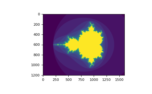
You can look at the following
example to see
how to use boolean indexing to generate an image of the Mandelbrot
set:
>>> import numpy as np
>>> import matplotlib.pyplot as plt
>>> def mandelbrot(h, w, maxit=20, r=2):
...     """Returns an image of the Mandelbrot fractal of size (h,w)."""
...     x = np.linspace(-2.5, 1.5, 4*h+1)
...     y = np.linspace(-1.5, 1.5, 3*w+1)
...     A, B = np.meshgrid(x, y)
...     C = A + B*1j
...     z = np.zeros_like(C)
...     divtime = maxit + np.zeros(z.shape, dtype=int)
...
...     for i in range(maxit):
...         z = z**2 + C
...         diverge = abs(z) > r                    # who is diverging
...         div_now = diverge & (divtime == maxit)  # who is diverging now
...         divtime[div_now] = i                    # note when
...         z[diverge] = r                          # avoid diverging too much
...
...     return divtime
>>> plt.clf()
>>> plt.imshow(mandelbrot(400, 400))
The second way of indexing with booleans is more similar to integer
indexing; for each dimension of the array we give a 1D boolean array
selecting the slices we want:
>>> a = np.arange(12).reshape(3, 4)
>>> b1 = np.array([False, True, True])         # first dim selection
>>> b2 = np.array([True, False, True, False])  # second dim selection
>>>
>>> a[b1, :]                                   # selecting rows
array([[ 4,  5,  6,  7],
       [ 8,  9, 10, 11]])
>>>
>>> a[b1]                                      # same thing
array([[ 4,  5,  6,  7],
       [ 8,  9, 10, 11]])
>>>
>>> a[:, b2]                                   # selecting columns
array([[ 0,  2],
       [ 4,  6],
       [ 8, 10]])
>>>
>>> a[b1, b2]                                  # a weird thing to do
array([ 4, 10])
Note that the length of the 1D boolean array must coincide with the
length of the dimension (or axis) you want to slice. In the previous
example, b1 has length 3 (the number of rows in a), and
b2 (of length 4) is suitable to index the 2nd axis (columns) of
a.
The ix_() function#
The ix_ function can be used to combine different vectors so as to
obtain the result for each n-uplet. For example, if you want to compute
all the a+b*c for all the triplets taken from each of the vectors a, b
and c:
>>> a = np.array([2, 3, 4, 5])
>>> b = np.array([8, 5, 4])
>>> c = np.array([5, 4, 6, 8, 3])
>>> ax, bx, cx = np.ix_(a, b, c)
>>> ax
array([[[2]],

       [[3]],

       [[4]],

       [[5]]])
>>> bx
array([[[8],
        [5],
        [4]]])
>>> cx
array([[[5, 4, 6, 8, 3]]])
>>> ax.shape, bx.shape, cx.shape
((4, 1, 1), (1, 3, 1), (1, 1, 5))
>>> result = ax + bx * cx
>>> result
array([[[42, 34, 50, 66, 26],
        [27, 22, 32, 42, 17],
        [22, 18, 26, 34, 14]],

       [[43, 35, 51, 67, 27],
        [28, 23, 33, 43, 18],
        [23, 19, 27, 35, 15]],

       [[44, 36, 52, 68, 28],
        [29, 24, 34, 44, 19],
        [24, 20, 28, 36, 16]],

       [[45, 37, 53, 69, 29],
        [30, 25, 35, 45, 20],
        [25, 21, 29, 37, 17]]])
>>> result[3, 2, 4]
17
>>> a[3] + b[2] * c[4]
17
You could also implement the reduce as follows:
>>> def ufunc_reduce(ufct, *vectors):
...    vs = np.ix_(*vectors)
...    r = ufct.identity
...    for v in vs:
...        r = ufct(r, v)
...    return r
and then use it as:
>>> ufunc_reduce(np.add, a, b, c)
array([[[15, 14, 16, 18, 13],
        [12, 11, 13, 15, 10],
        [11, 10, 12, 14,  9]],

       [[16, 15, 17, 19, 14],
        [13, 12, 14, 16, 11],
        [12, 11, 13, 15, 10]],

       [[17, 16, 18, 20, 15],
        [14, 13, 15, 17, 12],
        [13, 12, 14, 16, 11]],

       [[18, 17, 19, 21, 16],
        [15, 14, 16, 18, 13],
        [14, 13, 15, 17, 12]]])
The advantage of this version of reduce compared to the normal
ufunc.reduce is that it makes use of the
broadcasting rules
in order to avoid creating an argument array the size of the output
times the number of vectors.
Indexing with strings#
See Structured arrays.
Tricks and Tips#
Here we give a list of short and useful tips.
“Automatic” Reshaping#
To change the dimensions of an array, you can omit one of the sizes
which will then be deduced automatically:
>>> a = np.arange(30)
>>> b = a.reshape((2, -1, 3))  # -1 means "whatever is needed"
>>> b.shape
(2, 5, 3)
>>> b
array([[[ 0,  1,  2],
        [ 3,  4,  5],
        [ 6,  7,  8],
        [ 9, 10, 11],
        [12, 13, 14]],

       [[15, 16, 17],
        [18, 19, 20],
        [21, 22, 23],
        [24, 25, 26],
        [27, 28, 29]]])
Vector Stacking#
How do we construct a 2D array from a list of equally-sized row vectors?
In MATLAB this is quite easy: if x and y are two vectors of the
same length you only need do m=[x;y]. In NumPy this works via the
functions column_stack, dstack, hstack and vstack,
depending on the dimension in which the stacking is to be done. For
example:
>>> x = np.arange(0, 10, 2)
>>> y = np.arange(5)
>>> m = np.vstack([x, y])
>>> m
array([[0, 2, 4, 6, 8],
       [0, 1, 2, 3, 4]])
>>> xy = np.hstack([x, y])
>>> xy
array([0, 2, 4, 6, 8, 0, 1, 2, 3, 4])
The logic behind those functions in more than two dimensions can be
strange.
Histograms#
The NumPy histogram function applied to an array returns a pair of
vectors: the histogram of the array and a vector of the bin edges. Beware:
matplotlib also has a function to build histograms (called hist,
as in Matlab) that differs from the one in NumPy. The main difference is
that pylab.hist plots the histogram automatically, while
numpy.histogram only generates the data.
>>> import numpy as np
>>> rg = np.random.default_rng(1)
>>> import matplotlib.pyplot as plt
>>> # Build a vector of 10000 normal deviates with variance 0.5^2 and mean 2
>>> mu, sigma = 2, 0.5
>>> v = rg.normal(mu, sigma, 10000)
>>> # Plot a normalized histogram with 50 bins
>>> plt.hist(v, bins=50, density=True)       # matplotlib version (plot)
(array...)
>>> # Compute the histogram with numpy and then plot it
>>> (n, bins) = np.histogram(v, bins=50, density=True)  # NumPy version (no plot)
>>> plt.plot(.5 * (bins[1:] + bins[:-1]), n)
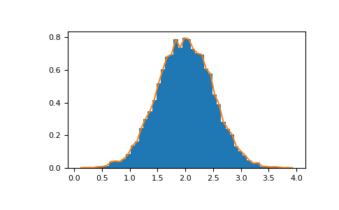
With Matplotlib >=3.4 you can also use plt.stairs(n, bins).
Further reading#
-
The Python tutorial
-
NumPy Reference
-
SciPy Tutorial
-
SciPy Lecture Notes
-
A matlab, R, IDL, NumPy/SciPy dictionary
-
tutorial-svd
Welcome to the absolute beginner’s guide to NumPy! If you have comments or
suggestions, please don’t hesitate to reach out!
Welcome to NumPy!#
NumPy (Numerical Python) is an open source Python library that’s used in
almost every field of science and engineering. It’s the universal standard for
working with numerical data in Python, and it’s at the core of the scientific
Python and PyData ecosystems. NumPy users include everyone from beginning coders
to experienced researchers doing state-of-the-art scientific and industrial
research and development. The NumPy API is used extensively in Pandas, SciPy,
Matplotlib, scikit-learn, scikit-image and most other data science and
scientific Python packages.
The NumPy library contains multidimensional array and matrix data structures
(you’ll find more information about this in later sections). It provides
ndarray, a homogeneous n-dimensional array object, with methods to
efficiently operate on it. NumPy can be used to perform a wide variety of
mathematical operations on arrays. It adds powerful data structures to Python
that guarantee efficient calculations with arrays and matrices and it supplies
an enormous library of high-level mathematical functions that operate on these
arrays and matrices.
Learn more about NumPy here!
Installing NumPy#
To install NumPy, we strongly recommend using a scientific Python distribution.
If you’re looking for the full instructions for installing NumPy on your
operating system, see Installing NumPy.
If you already have Python, you can install NumPy with:
or
If you don’t have Python yet, you might want to consider using Anaconda. It’s the easiest way to get started. The good
thing about getting this distribution is the fact that you don’t need to worry
too much about separately installing NumPy or any of the major packages that
you’ll be using for your data analyses, like pandas, Scikit-Learn, etc.
How to import NumPy#
To access NumPy and its functions import it in your Python code like this:
We shorten the imported name to np for better readability of code using
NumPy. This is a widely adopted convention that you should follow so that
anyone working with your code can easily understand it.
Reading the example code#
If you aren’t already comfortable with reading tutorials that contain a lot of code,
you might not know how to interpret a code block that looks
like this:
>>> a = np.arange(6)
>>> a2 = a[np.newaxis, :]
>>> a2.shape
(1, 6)
If you aren’t familiar with this style, it’s very easy to understand.
If you see >>>, you’re looking at input, or the code that
you would enter. Everything that doesn’t have >>> in front of it
is output, or the results of running your code. This is the style
you see when you run python on the command line, but if you’re using
IPython, you might see a different style. Note that it is not part of the
code and will cause an error if typed or pasted into the Python
shell. It can be safely typed or pasted into the IPython shell; the >>>
is ignored.
What’s the difference between a Python list and a NumPy array?#
NumPy gives you an enormous range of fast and efficient ways of creating arrays
and manipulating numerical data inside them. While a Python list can contain
different data types within a single list, all of the elements in a NumPy array
should be homogeneous. The mathematical operations that are meant to be performed
on arrays would be extremely inefficient if the arrays weren’t homogeneous.
Why use NumPy?
NumPy arrays are faster and more compact than Python lists. An array consumes
less memory and is convenient to use. NumPy uses much less memory to store data
and it provides a mechanism of specifying the data types. This allows the code
to be optimized even further.
What is an array?#
An array is a central data structure of the NumPy library. An array is a grid of
values and it contains information about the raw data, how to locate an element,
and how to interpret an element. It has a grid of elements that can be indexed
in various ways.
The elements are all of the same type, referred to as the array dtype.
An array can be indexed by a tuple of nonnegative integers, by booleans, by
another array, or by integers. The rank of the array is the number of
dimensions. The shape of the array is a tuple of integers giving the size of
the array along each dimension.
One way we can initialize NumPy arrays is from Python lists, using nested lists
for two- or higher-dimensional data.
For example:
>>> a = np.array([1, 2, 3, 4, 5, 6])
or:
>>> a = np.array([[1, 2, 3, 4], [5, 6, 7, 8], [9, 10, 11, 12]])
We can access the elements in the array using square brackets. When you’re
accessing elements, remember that indexing in NumPy starts at 0. That means that
if you want to access the first element in your array, you’ll be accessing
element “0”.
>>> print(a[0])
[1 2 3 4]
More information about arrays#
This section covers 1D array, 2D array, ndarray, vector, matrix
You might occasionally hear an array referred to as a “ndarray,” which is
shorthand for “N-dimensional array.” An N-dimensional array is simply an array
with any number of dimensions. You might also hear 1-D, or one-dimensional
array, 2-D, or two-dimensional array, and so on. The NumPy ndarray class
is used to represent both matrices and vectors. A vector is an array with a
single dimension (there’s no difference
between row and column vectors), while a matrix refers to an
array with two dimensions. For 3-D or higher dimensional arrays, the term
tensor is also commonly used.
What are the attributes of an array?
An array is usually a fixed-size container of items of the same type and size.
The number of dimensions and items in an array is defined by its shape. The
shape of an array is a tuple of non-negative integers that specify the sizes of
each dimension.
In NumPy, dimensions are called axes. This means that if you have a 2D array
that looks like this:
[[0., 0., 0.],
 [1., 1., 1.]]
Your array has 2 axes. The first axis has a length of 2 and the second axis has
a length of 3.
Just like in other Python container objects, the contents of an array can be
accessed and modified by indexing or slicing the array. Unlike the typical container
objects, different arrays can share the same data, so changes made on one array might
be visible in another.
Array attributes reflect information intrinsic to the array itself. If you
need to get, or even set, properties of an array without creating a new array,
you can often access an array through its attributes.
Read more about array attributes here and learn about
array objects here.
How to create a basic array#
This section covers np.array(), np.zeros(), np.ones(),
np.empty(), np.arange(), np.linspace(), dtype
To create a NumPy array, you can use the function np.array().
All you need to do to create a simple array is pass a list to it. If you choose
to, you can also specify the type of data in your list.
You can find more information about data types here.
>>> import numpy as np
>>> a = np.array([1, 2, 3])
You can visualize your array this way:

Be aware that these visualizations are meant to simplify ideas and give you a basic understanding of NumPy concepts and mechanics. Arrays and array operations are much more complicated than are captured here!
Besides creating an array from a sequence of elements, you can easily create an
array filled with 0’s:
>>> np.zeros(2)
array([0., 0.])
Or an array filled with 1’s:
>>> np.ones(2)
array([1., 1.])
Or even an empty array! The function empty creates an array whose initial
content is random and depends on the state of the memory. The reason to use
empty over zeros (or something similar) is speed — just make sure to
fill every element afterwards!
>>> # Create an empty array with 2 elements
>>> np.empty(2)
array([3.14, 42.  ])  # may vary
You can create an array with a range of elements:
>>> np.arange(4)
array([0, 1, 2, 3])
And even an array that contains a range of evenly spaced intervals. To do this,
you will specify the first number, last number, and the step size.
>>> np.arange(2, 9, 2)
array([2, 4, 6, 8])
You can also use np.linspace() to create an array with values that are
spaced linearly in a specified interval:
>>> np.linspace(0, 10, num=5)
array([ 0. ,  2.5,  5. ,  7.5, 10. ])
Specifying your data type
While the default data type is floating point (np.float64), you can explicitly
specify which data type you want using the dtype keyword.
>>> x = np.ones(2, dtype=np.int64)
>>> x
array([1, 1])
Learn more about creating arrays here
Adding, removing, and sorting elements#
This section covers np.sort(), np.concatenate()
Sorting an element is simple with np.sort(). You can specify the axis, kind,
and order when you call the function.
If you start with this array:
>>> arr = np.array([2, 1, 5, 3, 7, 4, 6, 8])
You can quickly sort the numbers in ascending order with:
>>> np.sort(arr)
array([1, 2, 3, 4, 5, 6, 7, 8])
In addition to sort, which returns a sorted copy of an array, you can use:
-
argsort, which is an indirect sort along a specified axis, -
lexsort, which is an indirect stable sort on multiple keys, -
searchsorted, which will find elements in a sorted array, and -
partition, which is a partial sort.
To read more about sorting an array, see: sort.
If you start with these arrays:
>>> a = np.array([1, 2, 3, 4])
>>> b = np.array([5, 6, 7, 8])
You can concatenate them with np.concatenate().
>>> np.concatenate((a, b))
array([1, 2, 3, 4, 5, 6, 7, 8])
Or, if you start with these arrays:
>>> x = np.array([[1, 2], [3, 4]])
>>> y = np.array([[5, 6]])
You can concatenate them with:
>>> np.concatenate((x, y), axis=0)
array([[1, 2],
       [3, 4],
       [5, 6]])
In order to remove elements from an array, it’s simple to use indexing to select
the elements that you want to keep.
To read more about concatenate, see: concatenate.
How do you know the shape and size of an array?#
This section covers ndarray.ndim, ndarray.size, ndarray.shape
ndarray.ndim will tell you the number of axes, or dimensions, of the array.
ndarray.size will tell you the total number of elements of the array. This
is the product of the elements of the array’s shape.
ndarray.shape will display a tuple of integers that indicate the number of
elements stored along each dimension of the array. If, for example, you have a
2-D array with 2 rows and 3 columns, the shape of your array is (2, 3).
For example, if you create this array:
>>> array_example = np.array([[[0, 1, 2, 3],
...                            [4, 5, 6, 7]],
...
...                           [[0, 1, 2, 3],
...                            [4, 5, 6, 7]],
...
...                           [[0 ,1 ,2, 3],
...                            [4, 5, 6, 7]]])
To find the number of dimensions of the array, run:
To find the total number of elements in the array, run:
>>> array_example.size
24
And to find the shape of your array, run:
>>> array_example.shape
(3, 2, 4)
Can you reshape an array?#
This section covers arr.reshape()
Yes!
Using arr.reshape() will give a new shape to an array without changing the
data. Just remember that when you use the reshape method, the array you want to
produce needs to have the same number of elements as the original array. If you
start with an array with 12 elements, you’ll need to make sure that your new
array also has a total of 12 elements.
If you start with this array:
>>> a = np.arange(6)
>>> print(a)
[0 1 2 3 4 5]
You can use reshape() to reshape your array. For example, you can reshape
this array to an array with three rows and two columns:
>>> b = a.reshape(3, 2)
>>> print(b)
[[0 1]
 [2 3]
 [4 5]]
With np.reshape, you can specify a few optional parameters:
>>> np.reshape(a, newshape=(1, 6), order='C')
array([[0, 1, 2, 3, 4, 5]])
a is the array to be reshaped.
newshape is the new shape you want. You can specify an integer or a tuple of
integers. If you specify an integer, the result will be an array of that length.
The shape should be compatible with the original shape.
order: C means to read/write the elements using C-like index order,
F means to read/write the elements using Fortran-like index order, A
means to read/write the elements in Fortran-like index order if a is Fortran
contiguous in memory, C-like order otherwise. (This is an optional parameter and
doesn’t need to be specified.)
If you want to learn more about C and Fortran order, you can
read more about the internal organization of NumPy arrays here.
Essentially, C and Fortran orders have to do with how indices correspond
to the order the array is stored in memory. In Fortran, when moving through
the elements of a two-dimensional array as it is stored in memory, the first
index is the most rapidly varying index. As the first index moves to the next
row as it changes, the matrix is stored one column at a time.
This is why Fortran is thought of as a Column-major language.
In C on the other hand, the last index changes
the most rapidly. The matrix is stored by rows, making it a Row-major
language. What you do for C or Fortran depends on whether it’s more important
to preserve the indexing convention or not reorder the data.
Learn more about shape manipulation here.
How to convert a 1D array into a 2D array (how to add a new axis to an array)#
This section covers np.newaxis, np.expand_dims
You can use np.newaxis and np.expand_dims to increase the dimensions of
your existing array.
Using np.newaxis will increase the dimensions of your array by one dimension
when used once. This means that a 1D array will become a 2D array, a
2D array will become a 3D array, and so on.
For example, if you start with this array:
>>> a = np.array([1, 2, 3, 4, 5, 6])
>>> a.shape
(6,)
You can use np.newaxis to add a new axis:
>>> a2 = a[np.newaxis, :]
>>> a2.shape
(1, 6)
You can explicitly convert a 1D array with either a row vector or a column
vector using np.newaxis. For example, you can convert a 1D array to a row
vector by inserting an axis along the first dimension:
>>> row_vector = a[np.newaxis, :]
>>> row_vector.shape
(1, 6)
Or, for a column vector, you can insert an axis along the second dimension:
>>> col_vector = a[:, np.newaxis]
>>> col_vector.shape
(6, 1)
You can also expand an array by inserting a new axis at a specified position
with np.expand_dims.
For example, if you start with this array:
>>> a = np.array([1, 2, 3, 4, 5, 6])
>>> a.shape
(6,)
You can use np.expand_dims to add an axis at index position 1 with:
>>> b = np.expand_dims(a, axis=1)
>>> b.shape
(6, 1)
You can add an axis at index position 0 with:
>>> c = np.expand_dims(a, axis=0)
>>> c.shape
(1, 6)
Find more information about newaxis here and
expand_dims at expand_dims.
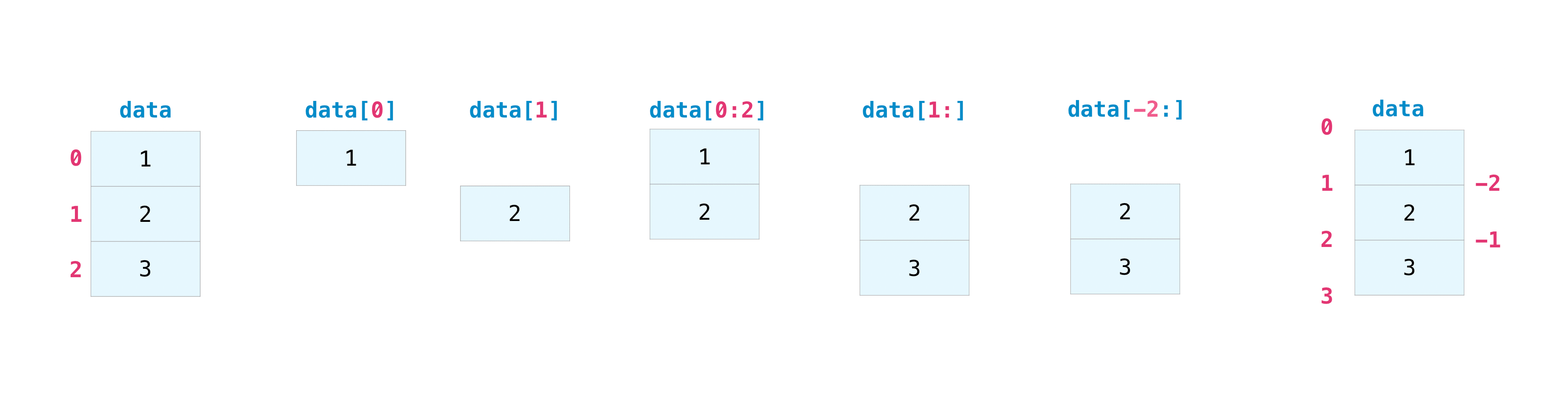
Indexing and slicing#
You can index and slice NumPy arrays in the same ways you can slice Python
lists.
>>> data = np.array([1, 2, 3])

>>> data[1]
2
>>> data[0:2]
array([1, 2])
>>> data[1:]
array([2, 3])
>>> data[-2:]
array([2, 3])
You can visualize it this way:
You may want to take a section of your array or specific array elements to use
in further analysis or additional operations. To do that, you’ll need to subset,
slice, and/or index your arrays.
If you want to select values from your array that fulfill certain conditions,
it’s straightforward with NumPy.
For example, if you start with this array:
>>> a = np.array([[1 , 2, 3, 4], [5, 6, 7, 8], [9, 10, 11, 12]])
You can easily print all of the values in the array that are less than 5.
>>> print(a[a < 5])
[1 2 3 4]
You can also select, for example, numbers that are equal to or greater than 5,
and use that condition to index an array.
>>> five_up = (a >= 5)
>>> print(a[five_up])
[ 5  6  7  8  9 10 11 12]
You can select elements that are divisible by 2:
>>> divisible_by_2 = a[a%2==0]
>>> print(divisible_by_2)
[ 2  4  6  8 10 12]
Or you can select elements that satisfy two conditions using the & and |
operators:
>>> c = a[(a > 2) & (a < 11)]
>>> print(c)
[ 3  4  5  6  7  8  9 10]
You can also make use of the logical operators & and | in order to
return boolean values that specify whether or not the values in an array fulfill
a certain condition. This can be useful with arrays that contain names or other
categorical values.
>>> five_up = (a > 5) | (a == 5)
>>> print(five_up)
[[False False False False]
 [ True  True  True  True]
 [ True  True  True True]]
You can also use np.nonzero() to select elements or indices from an array.
Starting with this array:
>>> a = np.array([[1, 2, 3, 4], [5, 6, 7, 8], [9, 10, 11, 12]])
You can use np.nonzero() to print the indices of elements that are, for
example, less than 5:
>>> b = np.nonzero(a < 5)
>>> print(b)
(array([0, 0, 0, 0]), array([0, 1, 2, 3]))
In this example, a tuple of arrays was returned: one for each dimension. The
first array represents the row indices where these values are found, and the
second array represents the column indices where the values are found.
If you want to generate a list of coordinates where the elements exist, you can
zip the arrays, iterate over the list of coordinates, and print them. For
example:
>>> list_of_coordinates= list(zip(b[0], b[1]))

>>> for coord in list_of_coordinates:
...     print(coord)
(0, 0)
(0, 1)
(0, 2)
(0, 3)
You can also use np.nonzero() to print the elements in an array that are less
than 5 with:
>>> print(a[b])
[1 2 3 4]
If the element you’re looking for doesn’t exist in the array, then the returned
array of indices will be empty. For example:
>>> not_there = np.nonzero(a == 42)
>>> print(not_there)
(array([], dtype=int64), array([], dtype=int64))
Learn more about indexing and slicing here
and here.
Read more about using the nonzero function at: nonzero.
How to create an array from existing data#
This section covers slicing and indexing, np.vstack(), np.hstack(),
np.hsplit(), .view(), copy()
You can easily create a new array from a section of an existing array.
Let’s say you have this array:
>>> a = np.array([1, 2, 3, 4, 5, 6, 7, 8, 9, 10])
You can create a new array from a section of your array any time by specifying
where you want to slice your array.
>>> arr1 = a[3:8]
>>> arr1
array([4, 5, 6, 7, 8])
Here, you grabbed a section of your array from index position 3 through index
position 8.
You can also stack two existing arrays, both vertically and horizontally. Let’s
say you have two arrays, a1 and a2:
>>> a1 = np.array([[1, 1],
...                [2, 2]])

>>> a2 = np.array([[3, 3],
...                [4, 4]])
You can stack them vertically with vstack:
>>> np.vstack((a1, a2))
array([[1, 1],
       [2, 2],
       [3, 3],
       [4, 4]])
Or stack them horizontally with hstack:
>>> np.hstack((a1, a2))
array([[1, 1, 3, 3],
       [2, 2, 4, 4]])
You can split an array into several smaller arrays using hsplit. You can
specify either the number of equally shaped arrays to return or the columns
after which the division should occur.
Let’s say you have this array:
>>> x = np.arange(1, 25).reshape(2, 12)
>>> x
array([[ 1,  2,  3,  4,  5,  6,  7,  8,  9, 10, 11, 12],
       [13, 14, 15, 16, 17, 18, 19, 20, 21, 22, 23, 24]])
If you wanted to split this array into three equally shaped arrays, you would
run:
>>> np.hsplit(x, 3)
  [array([[ 1,  2,  3,  4],
         [13, 14, 15, 16]]), array([[ 5,  6,  7,  8],
         [17, 18, 19, 20]]), array([[ 9, 10, 11, 12],
         [21, 22, 23, 24]])]
If you wanted to split your array after the third and fourth column, you’d run:
>>> np.hsplit(x, (3, 4))
  [array([[ 1,  2,  3],
         [13, 14, 15]]), array([[ 4],
         [16]]), array([[ 5,  6,  7,  8,  9, 10, 11, 12],
         [17, 18, 19, 20, 21, 22, 23, 24]])]
Learn more about stacking and splitting arrays here.
You can use the view method to create a new array object that looks at the
same data as the original array (a shallow copy).
Views are an important NumPy concept! NumPy functions, as well as operations
like indexing and slicing, will return views whenever possible. This saves
memory and is faster (no copy of the data has to be made). However it’s
important to be aware of this — modifying data in a view also modifies the
original array!
Let’s say you create this array:
>>> a = np.array([[1, 2, 3, 4], [5, 6, 7, 8], [9, 10, 11, 12]])
Now we create an array b1 by slicing a and modify the first element of
b1. This will modify the corresponding element in a as well!
>>> b1 = a[0, :]
>>> b1
array([1, 2, 3, 4])
>>> b1[0] = 99
>>> b1
array([99,  2,  3,  4])
>>> a
array([[99,  2,  3,  4],
       [ 5,  6,  7,  8],
       [ 9, 10, 11, 12]])
Using the copy method will make a complete copy of the array and its data (a
deep copy). To use this on your array, you could run:
Learn more about copies and views here.
Basic array operations#
This section covers addition, subtraction, multiplication, division, and more
Once you’ve created your arrays, you can start to work with them. Let’s say,
for example, that you’ve created two arrays, one called “data” and one called
“ones”
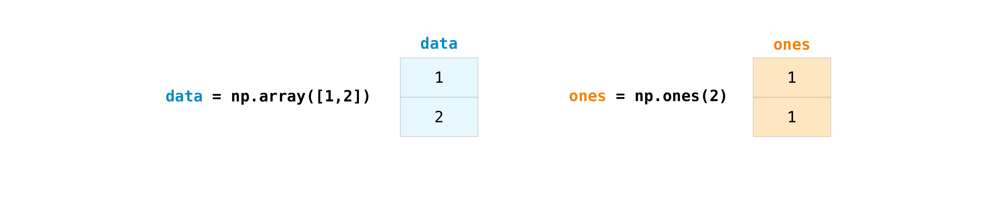
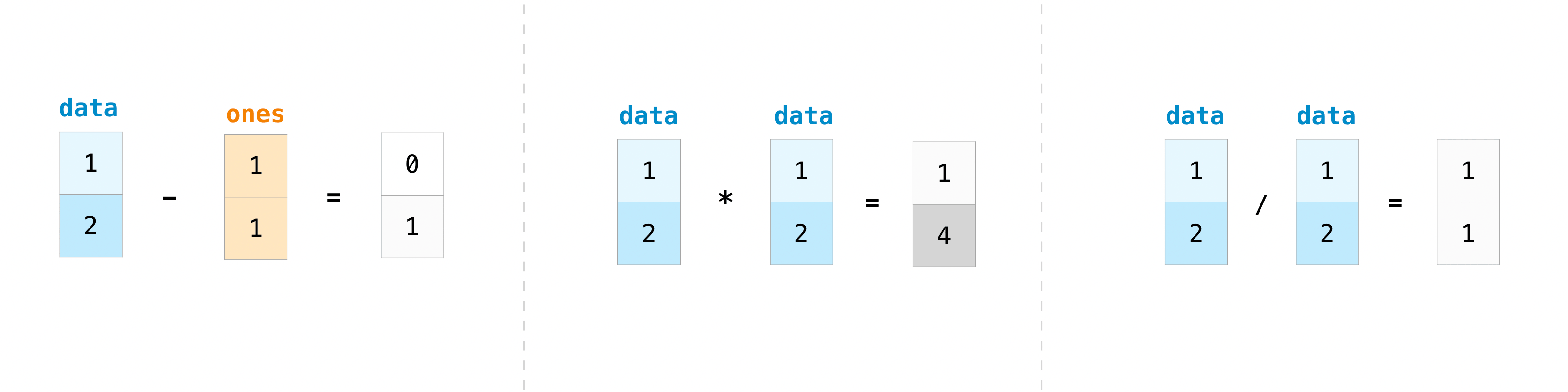
You can add the arrays together with the plus sign.
>>> data = np.array([1, 2])
>>> ones = np.ones(2, dtype=int)
>>> data + ones
array([2, 3])

You can, of course, do more than just addition!
>>> data - ones
array([0, 1])
>>> data * data
array([1, 4])
>>> data / data
array([1., 1.])
Basic operations are simple with NumPy. If you want to find the sum of the
elements in an array, you’d use sum(). This works for 1D arrays, 2D arrays,
and arrays in higher dimensions.
>>> a = np.array([1, 2, 3, 4])

>>> a.sum()
10
To add the rows or the columns in a 2D array, you would specify the axis.
If you start with this array:
>>> b = np.array([[1, 1], [2, 2]])
You can sum over the axis of rows with:
>>> b.sum(axis=0)
array([3, 3])
You can sum over the axis of columns with:
>>> b.sum(axis=1)
array([2, 4])
Learn more about basic operations here.
Broadcasting#
There are times when you might want to carry out an operation between an array
and a single number (also called an operation between a vector and a scalar)
or between arrays of two different sizes. For example, your array (we’ll call it
“data”) might contain information about distance in miles but you want to
convert the information to kilometers. You can perform this operation with:
>>> data = np.array([1.0, 2.0])
>>> data * 1.6
array([1.6, 3.2])
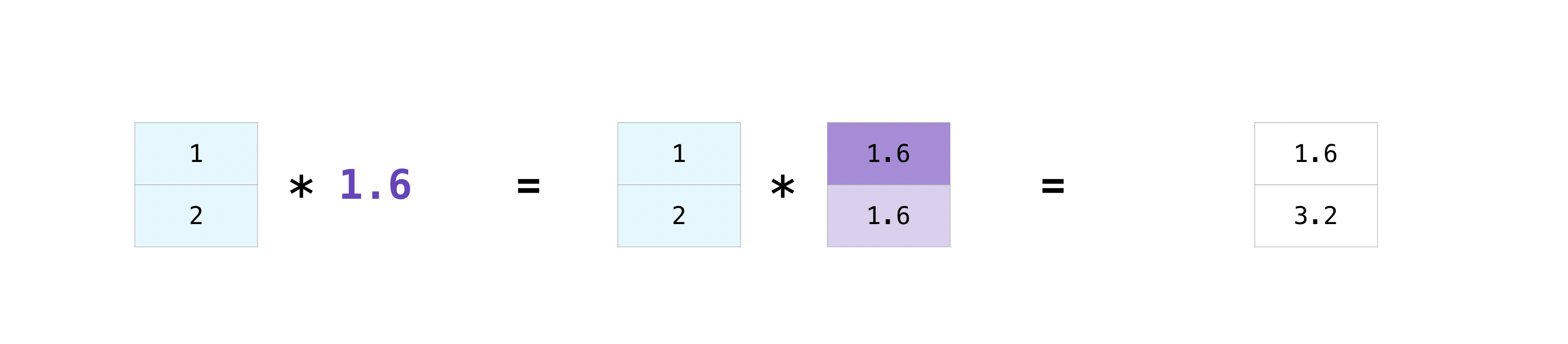
NumPy understands that the multiplication should happen with each cell. That
concept is called broadcasting. Broadcasting is a mechanism that allows
NumPy to perform operations on arrays of different shapes. The dimensions of
your array must be compatible, for example, when the dimensions of both arrays
are equal or when one of them is 1. If the dimensions are not compatible, you
will get a ValueError.
Learn more about broadcasting here.
More useful array operations#
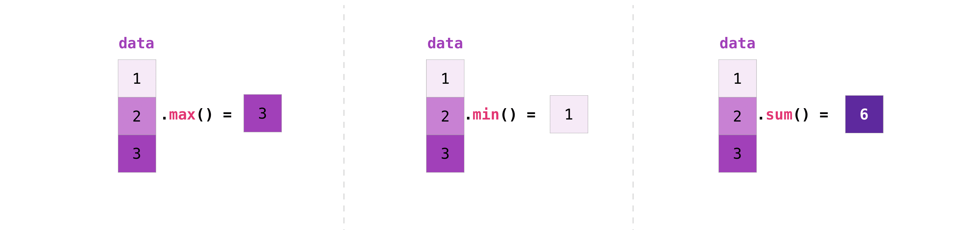
This section covers maximum, minimum, sum, mean, product, standard deviation, and more
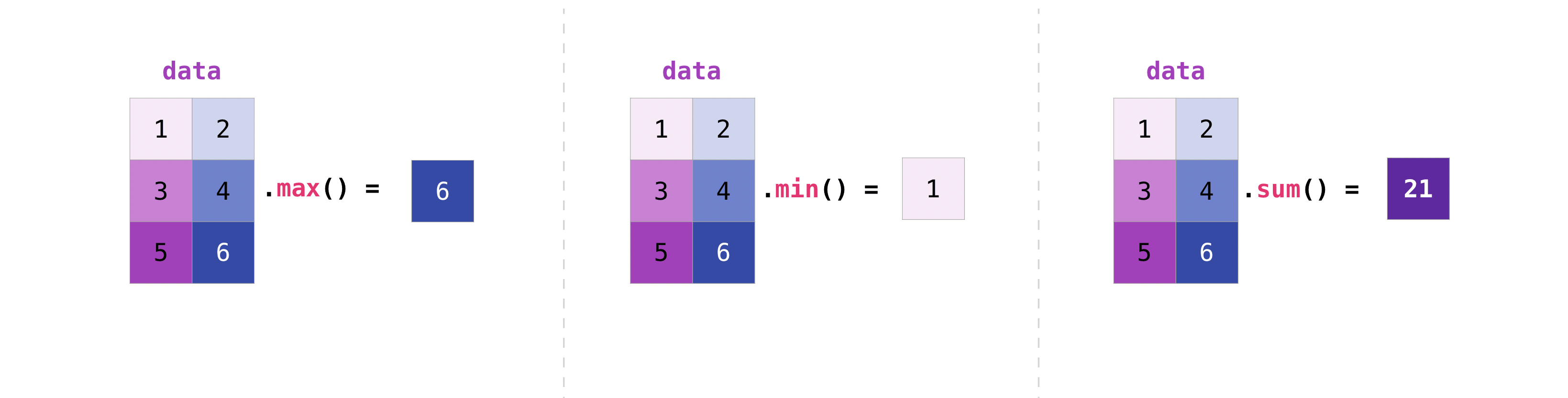
NumPy also performs aggregation functions. In addition to min, max, and
sum, you can easily run mean to get the average, prod to get the
result of multiplying the elements together, std to get the standard
deviation, and more.
>>> data.max()
2.0
>>> data.min()
1.0
>>> data.sum()
3.0
Let’s start with this array, called “a”
>>> a = np.array([[0.45053314, 0.17296777, 0.34376245, 0.5510652],
...               [0.54627315, 0.05093587, 0.40067661, 0.55645993],
...               [0.12697628, 0.82485143, 0.26590556, 0.56917101]])
It’s very common to want to aggregate along a row or column. By default, every
NumPy aggregation function will return the aggregate of the entire array. To
find the sum or the minimum of the elements in your array, run:
Or:
You can specify on which axis you want the aggregation function to be computed.
For example, you can find the minimum value within each column by specifying
axis=0.
>>> a.min(axis=0)
array([0.12697628, 0.05093587, 0.26590556, 0.5510652 ])
The four values listed above correspond to the number of columns in your array.
With a four-column array, you will get four values as your result.
Read more about array methods here.
Creating matrices#
You can pass Python lists of lists to create a 2-D array (or “matrix”) to
represent them in NumPy.
>>> data = np.array([[1, 2], [3, 4], [5, 6]])
>>> data
array([[1, 2],
       [3, 4],
       [5, 6]])

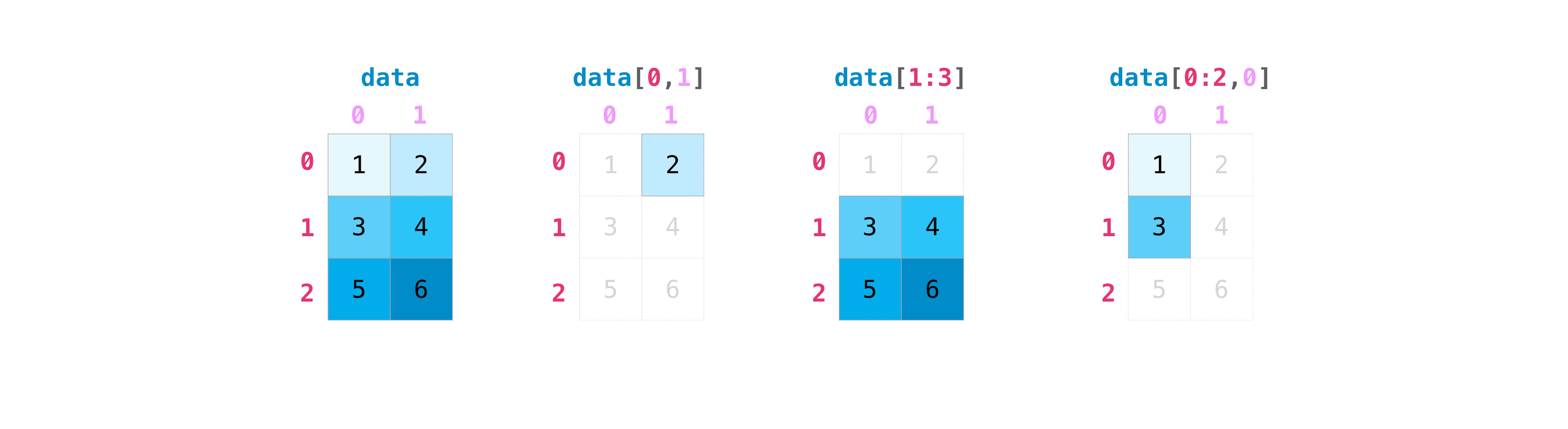
Indexing and slicing operations are useful when you’re manipulating matrices:
>>> data[0, 1]
2
>>> data[1:3]
array([[3, 4],
       [5, 6]])
>>> data[0:2, 0]
array([1, 3])
You can aggregate matrices the same way you aggregated vectors:
>>> data.max()
6
>>> data.min()
1
>>> data.sum()
21
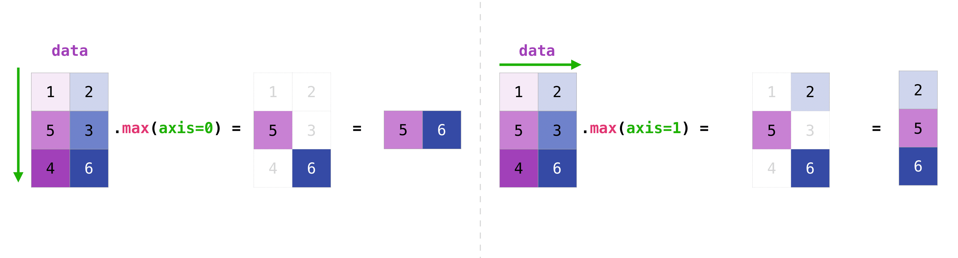
You can aggregate all the values in a matrix and you can aggregate them across
columns or rows using the axis parameter. To illustrate this point, let’s
look at a slightly modified dataset:
>>> data = np.array([[1, 2], [5, 3], [4, 6]])
>>> data
array([[1, 2],
       [5, 3],
       [4, 6]])
>>> data.max(axis=0)
array([5, 6])
>>> data.max(axis=1)
array([2, 5, 6])
Once you’ve created your matrices, you can add and multiply them using
arithmetic operators if you have two matrices that are the same size.
>>> data = np.array([[1, 2], [3, 4]])
>>> ones = np.array([[1, 1], [1, 1]])
>>> data + ones
array([[2, 3],
       [4, 5]])

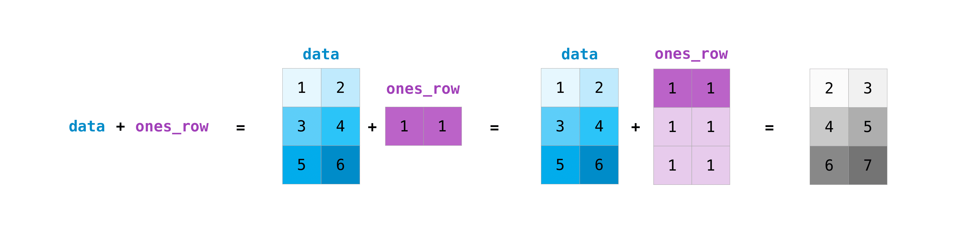
You can do these arithmetic operations on matrices of different sizes, but only
if one matrix has only one column or one row. In this case, NumPy will use its
broadcast rules for the operation.
>>> data = np.array([[1, 2], [3, 4], [5, 6]])
>>> ones_row = np.array([[1, 1]])
>>> data + ones_row
array([[2, 3],
       [4, 5],
       [6, 7]])
Be aware that when NumPy prints N-dimensional arrays, the last axis is looped
over the fastest while the first axis is the slowest. For instance:
>>> np.ones((4, 3, 2))
array([[[1., 1.],
        [1., 1.],
        [1., 1.]],

       [[1., 1.],
        [1., 1.],
        [1., 1.]],

       [[1., 1.],
        [1., 1.],
        [1., 1.]],

       [[1., 1.],
        [1., 1.],
        [1., 1.]]])
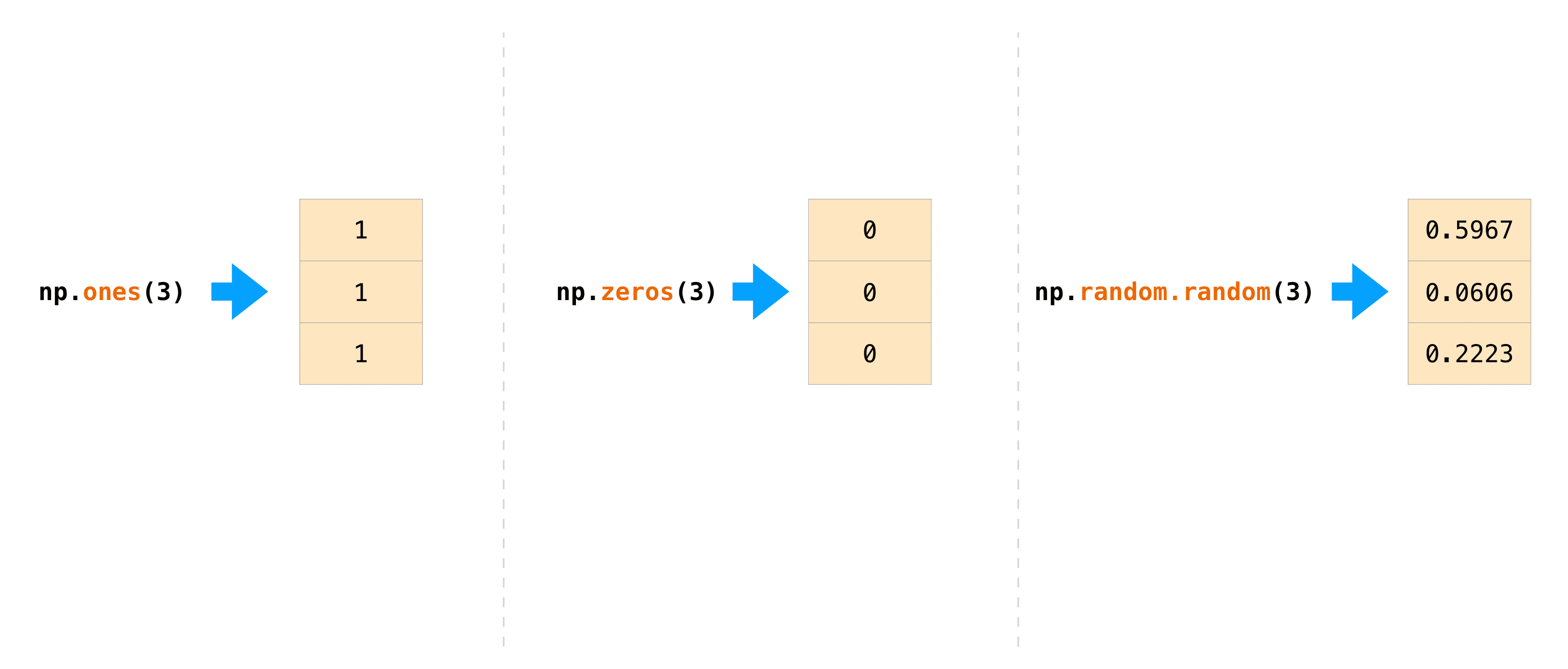
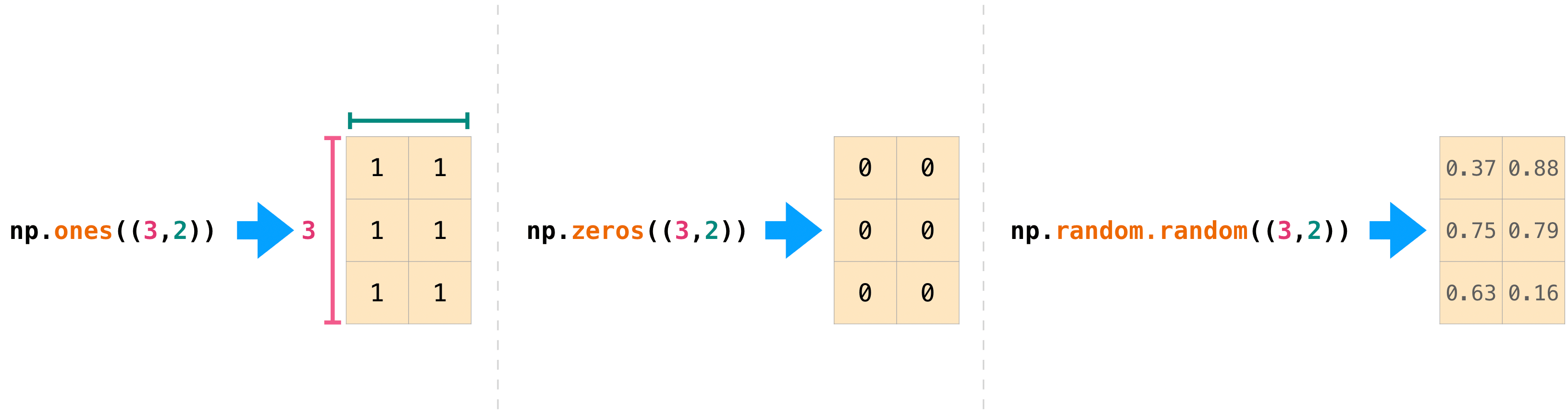
There are often instances where we want NumPy to initialize the values of an
array. NumPy offers functions like ones() and zeros(), and the
random.Generator class for random number generation for that.
All you need to do is pass in the number of elements you want it to generate:
>>> np.ones(3)
array([1., 1., 1.])
>>> np.zeros(3)
array([0., 0., 0.])
>>> rng = np.random.default_rng()  # the simplest way to generate random numbers
>>> rng.random(3)
array([0.63696169, 0.26978671, 0.04097352])
You can also use ones(), zeros(), and random() to create
a 2D array if you give them a tuple describing the dimensions of the matrix:
>>> np.ones((3, 2))
array([[1., 1.],
       [1., 1.],
       [1., 1.]])
>>> np.zeros((3, 2))
array([[0., 0.],
       [0., 0.],
       [0., 0.]])
>>> rng.random((3, 2))
array([[0.01652764, 0.81327024],
       [0.91275558, 0.60663578],
       [0.72949656, 0.54362499]])  # may vary
Read more about creating arrays, filled with 0’s, 1’s, other values or
uninitialized, at array creation routines.
Generating random numbers#
The use of random number generation is an important part of the configuration
and evaluation of many numerical and machine learning algorithms. Whether you
need to randomly initialize weights in an artificial neural network, split data
into random sets, or randomly shuffle your dataset, being able to generate
random numbers (actually, repeatable pseudo-random numbers) is essential.
With Generator.integers, you can generate random integers from low (remember
that this is inclusive with NumPy) to high (exclusive). You can set
endpoint=True to make the high number inclusive.
You can generate a 2 x 4 array of random integers between 0 and 4 with:
>>> rng.integers(5, size=(2, 4))
array([[2, 1, 1, 0],
       [0, 0, 0, 4]])  # may vary
Read more about random number generation here.
How to get unique items and counts#
This section covers np.unique()
You can find the unique elements in an array easily with np.unique.
For example, if you start with this array:
>>> a = np.array([11, 11, 12, 13, 14, 15, 16, 17, 12, 13, 11, 14, 18, 19, 20])
you can use np.unique to print the unique values in your array:
>>> unique_values = np.unique(a)
>>> print(unique_values)
[11 12 13 14 15 16 17 18 19 20]
To get the indices of unique values in a NumPy array (an array of first index
positions of unique values in the array), just pass the return_index
argument in np.unique() as well as your array.
>>> unique_values, indices_list = np.unique(a, return_index=True)
>>> print(indices_list)
[ 0  2  3  4  5  6  7 12 13 14]
You can pass the return_counts argument in np.unique() along with your
array to get the frequency count of unique values in a NumPy array.
>>> unique_values, occurrence_count = np.unique(a, return_counts=True)
>>> print(occurrence_count)
[3 2 2 2 1 1 1 1 1 1]
This also works with 2D arrays!
If you start with this array:
>>> a_2d = np.array([[1, 2, 3, 4], [5, 6, 7, 8], [9, 10, 11, 12], [1, 2, 3, 4]])
You can find unique values with:
>>> unique_values = np.unique(a_2d)
>>> print(unique_values)
[ 1  2  3  4  5  6  7  8  9 10 11 12]
If the axis argument isn’t passed, your 2D array will be flattened.
If you want to get the unique rows or columns, make sure to pass the axis
argument. To find the unique rows, specify axis=0 and for columns, specify
axis=1.
>>> unique_rows = np.unique(a_2d, axis=0)
>>> print(unique_rows)
[[ 1  2  3  4]
 [ 5  6  7  8]
 [ 9 10 11 12]]
To get the unique rows, index position, and occurrence count, you can use:
>>> unique_rows, indices, occurrence_count = np.unique(
...      a_2d, axis=0, return_counts=True, return_index=True)
>>> print(unique_rows)
[[ 1  2  3  4]
 [ 5  6  7  8]
 [ 9 10 11 12]]
>>> print(indices)
[0 1 2]
>>> print(occurrence_count)
[2 1 1]
To learn more about finding the unique elements in an array, see unique.
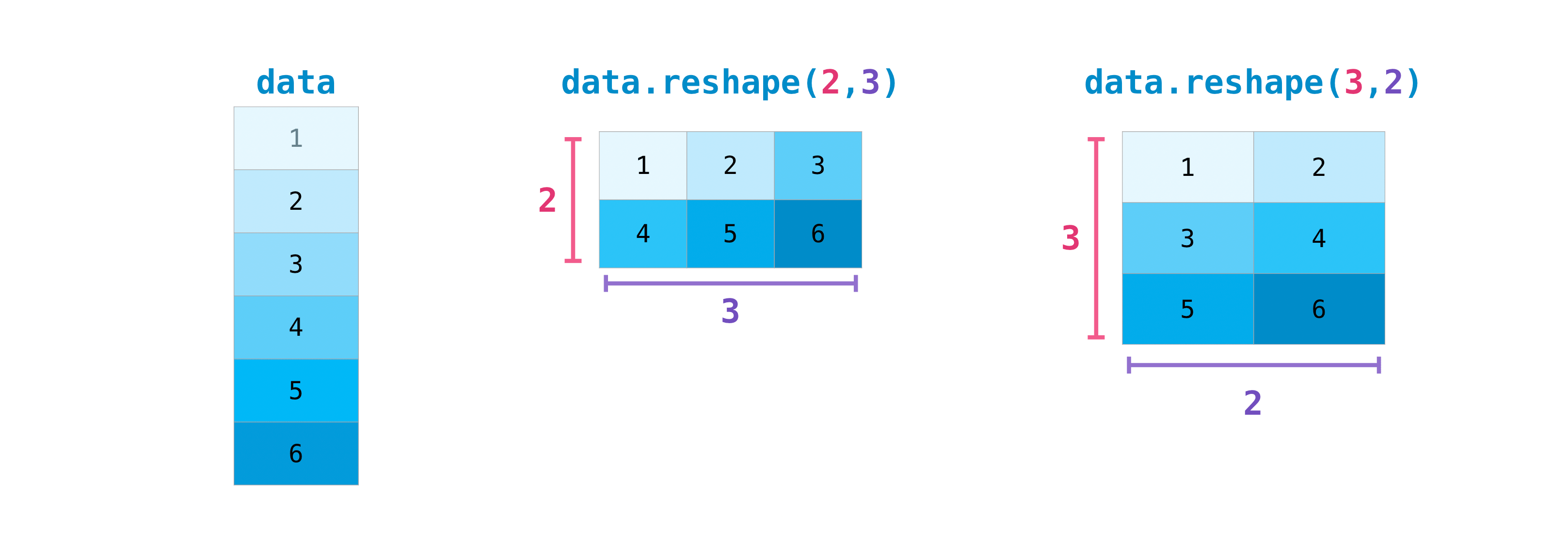
Transposing and reshaping a matrix#
This section covers arr.reshape(), arr.transpose(), arr.T
It’s common to need to transpose your matrices. NumPy arrays have the property
T that allows you to transpose a matrix.

You may also need to switch the dimensions of a matrix. This can happen when,
for example, you have a model that expects a certain input shape that is
different from your dataset. This is where the reshape method can be useful.
You simply need to pass in the new dimensions that you want for the matrix.
>>> data.reshape(2, 3)
array([[1, 2, 3],
       [4, 5, 6]])
>>> data.reshape(3, 2)
array([[1, 2],
       [3, 4],
       [5, 6]])
You can also use .transpose() to reverse or change the axes of an array
according to the values you specify.
If you start with this array:
>>> arr = np.arange(6).reshape((2, 3))
>>> arr
array([[0, 1, 2],
       [3, 4, 5]])
You can transpose your array with arr.transpose().
>>> arr.transpose()
array([[0, 3],
       [1, 4],
       [2, 5]])
You can also use arr.T:
>>> arr.T
array([[0, 3],
       [1, 4],
       [2, 5]])
To learn more about transposing and reshaping arrays, see transpose and
reshape.
How to reverse an array#
This section covers np.flip()
NumPy’s np.flip() function allows you to flip, or reverse, the contents of
an array along an axis. When using np.flip(), specify the array you would like
to reverse and the axis. If you don’t specify the axis, NumPy will reverse the
contents along all of the axes of your input array.
Reversing a 1D array
If you begin with a 1D array like this one:
>>> arr = np.array([1, 2, 3, 4, 5, 6, 7, 8])
You can reverse it with:
>>> reversed_arr = np.flip(arr)
If you want to print your reversed array, you can run:
>>> print('Reversed Array: ', reversed_arr)
Reversed Array:  [8 7 6 5 4 3 2 1]
Reversing a 2D array
A 2D array works much the same way.
If you start with this array:
>>> arr_2d = np.array([[1, 2, 3, 4], [5, 6, 7, 8], [9, 10, 11, 12]])
You can reverse the content in all of the rows and all of the columns with:
>>> reversed_arr = np.flip(arr_2d)
>>> print(reversed_arr)
[[12 11 10  9]
 [ 8  7  6  5]
 [ 4  3  2  1]]
You can easily reverse only the rows with:
>>> reversed_arr_rows = np.flip(arr_2d, axis=0)
>>> print(reversed_arr_rows)
[[ 9 10 11 12]
 [ 5  6  7  8]
 [ 1  2  3  4]]
Or reverse only the columns with:
>>> reversed_arr_columns = np.flip(arr_2d, axis=1)
>>> print(reversed_arr_columns)
[[ 4  3  2  1]
 [ 8  7  6  5]
 [12 11 10  9]]
You can also reverse the contents of only one column or row. For example, you
can reverse the contents of the row at index position 1 (the second row):
>>> arr_2d[1] = np.flip(arr_2d[1])
>>> print(arr_2d)
[[ 1  2  3  4]
 [ 8  7  6  5]
 [ 9 10 11 12]]
You can also reverse the column at index position 1 (the second column):
>>> arr_2d[:,1] = np.flip(arr_2d[:,1])
>>> print(arr_2d)
[[ 1 10  3  4]
 [ 8  7  6  5]
 [ 9  2 11 12]]
Read more about reversing arrays at flip.
Reshaping and flattening multidimensional arrays#
This section covers .flatten(), ravel()
There are two popular ways to flatten an array: .flatten() and .ravel().
The primary difference between the two is that the new array created using
ravel() is actually a reference to the parent array (i.e., a “view”). This
means that any changes to the new array will affect the parent array as well.
Since ravel does not create a copy, it’s memory efficient.
If you start with this array:
>>> x = np.array([[1 , 2, 3, 4], [5, 6, 7, 8], [9, 10, 11, 12]])
You can use flatten to flatten your array into a 1D array.
>>> x.flatten()
array([ 1,  2,  3,  4,  5,  6,  7,  8,  9, 10, 11, 12])
When you use flatten, changes to your new array won’t change the parent
array.
For example:
>>> a1 = x.flatten()
>>> a1[0] = 99
>>> print(x)  # Original array
[[ 1  2  3  4]
 [ 5  6  7  8]
 [ 9 10 11 12]]
>>> print(a1)  # New array
[99  2  3  4  5  6  7  8  9 10 11 12]
But when you use ravel, the changes you make to the new array will affect
the parent array.
For example:
>>> a2 = x.ravel()
>>> a2[0] = 98
>>> print(x)  # Original array
[[98  2  3  4]
 [ 5  6  7  8]
 [ 9 10 11 12]]
>>> print(a2)  # New array
[98  2  3  4  5  6  7  8  9 10 11 12]
Read more about flatten at ndarray.flatten and ravel at ravel.
How to access the docstring for more information#
This section covers help(), ?, ??
When it comes to the data science ecosystem, Python and NumPy are built with the
user in mind. One of the best examples of this is the built-in access to
documentation. Every object contains the reference to a string, which is known
as the docstring. In most cases, this docstring contains a quick and concise
summary of the object and how to use it. Python has a built-in help()
function that can help you access this information. This means that nearly any
time you need more information, you can use help() to quickly find the
information that you need.
For example:
>>> help(max)
Help on built-in function max in module builtins:

max(...)
    max(iterable, *[, default=obj, key=func]) -> value
    max(arg1, arg2, *args, *[, key=func]) -> value

    With a single iterable argument, return its biggest item. The
    default keyword-only argument specifies an object to return if
    the provided iterable is empty.
    With two or more arguments, return the largest argument.
Because access to additional information is so useful, IPython uses the ?
character as a shorthand for accessing this documentation along with other
relevant information. IPython is a command shell for interactive computing in
multiple languages.
You can find more information about IPython here.
For example:
In [0]: max?
max(iterable, *[, default=obj, key=func]) -> value
max(arg1, arg2, *args, *[, key=func]) -> value

With a single iterable argument, return its biggest item. The
default keyword-only argument specifies an object to return if
the provided iterable is empty.
With two or more arguments, return the largest argument.
Type:      builtin_function_or_method
You can even use this notation for object methods and objects themselves.
Let’s say you create this array:
>>> a = np.array([1, 2, 3, 4, 5, 6])
Then you can obtain a lot of useful information (first details about a itself,
followed by the docstring of ndarray of which a is an instance):
In [1]: a?
Type:            ndarray
String form:     [1 2 3 4 5 6]
Length:          6
File:            ~/anaconda3/lib/python3.9/site-packages/numpy/__init__.py
Docstring:       <no docstring>
Class docstring:
ndarray(shape, dtype=float, buffer=None, offset=0,
        strides=None, order=None)

An array object represents a multidimensional, homogeneous array
of fixed-size items.  An associated data-type object describes the
format of each element in the array (its byte-order, how many bytes it
occupies in memory, whether it is an integer, a floating point number,
or something else, etc.)

Arrays should be constructed using `array`, `zeros` or `empty` (refer
to the See Also section below).  The parameters given here refer to
a low-level method (`ndarray(...)`) for instantiating an array.

For more information, refer to the `numpy` module and examine the
methods and attributes of an array.

Parameters
----------
(for the __new__ method; see Notes below)

shape : tuple of ints
        Shape of created array.
...
This also works for functions and other objects that you create. Just
remember to include a docstring with your function using a string literal
(""" """ or ''' ''' around your documentation).
For example, if you create this function:
>>> def double(a):
...   '''Return a * 2'''
...   return a * 2
You can obtain information about the function:
In [2]: double?
Signature: double(a)
Docstring: Return a * 2
File:      ~/Desktop/<ipython-input-23-b5adf20be596>
Type:      function
You can reach another level of information by reading the source code of the
object you’re interested in. Using a double question mark (??) allows you to
access the source code.
For example:
In [3]: double??
Signature: double(a)
Source:
def double(a):
    '''Return a * 2'''
    return a * 2
File:      ~/Desktop/<ipython-input-23-b5adf20be596>
Type:      function
If the object in question is compiled in a language other than Python, using
?? will return the same information as ?. You’ll find this with a lot of
built-in objects and types, for example:
In [4]: len?
Signature: len(obj, /)
Docstring: Return the number of items in a container.
Type:      builtin_function_or_method
and :
In [5]: len??
Signature: len(obj, /)
Docstring: Return the number of items in a container.
Type:      builtin_function_or_method
have the same output because they were compiled in a programming language other
than Python.
Working with mathematical formulas#
The ease of implementing mathematical formulas that work on arrays is one of
the things that make NumPy so widely used in the scientific Python community.
For example, this is the mean square error formula (a central formula used in
supervised machine learning models that deal with regression):
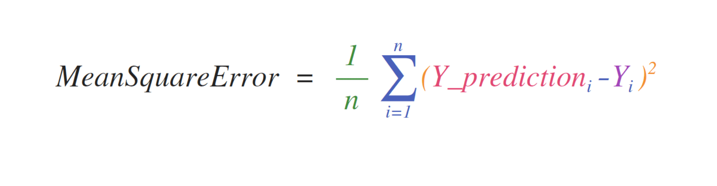
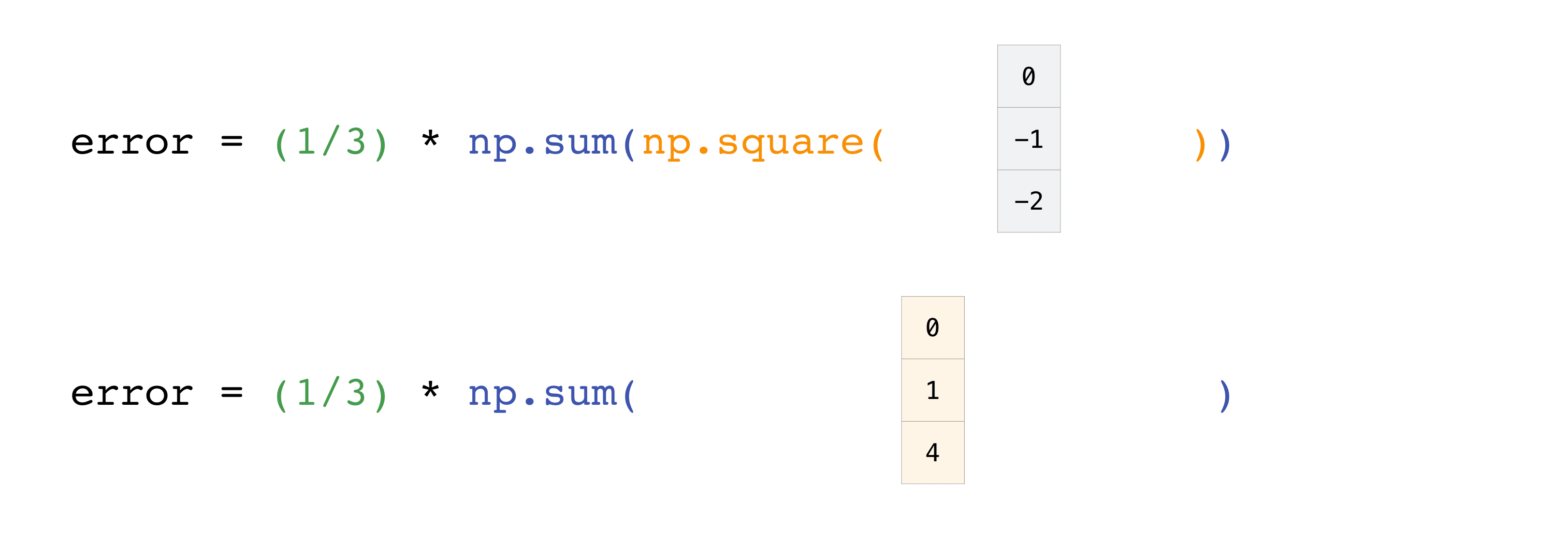
Implementing this formula is simple and straightforward in NumPy:
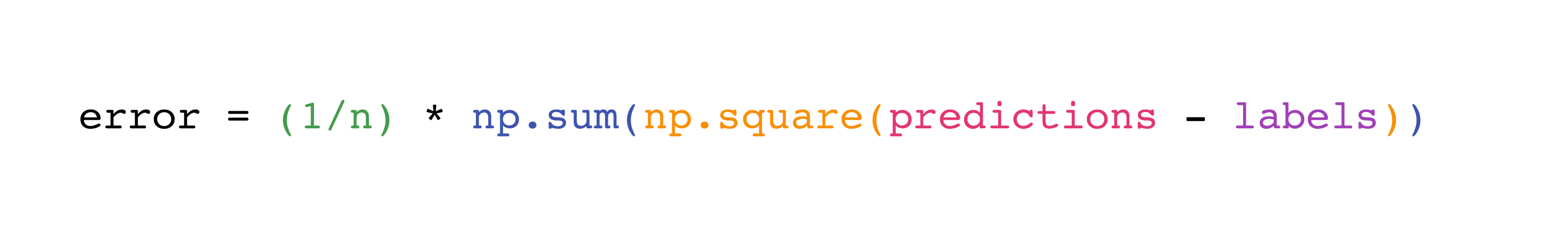
What makes this work so well is that predictions and labels can contain
one or a thousand values. They only need to be the same size.
You can visualize it this way:
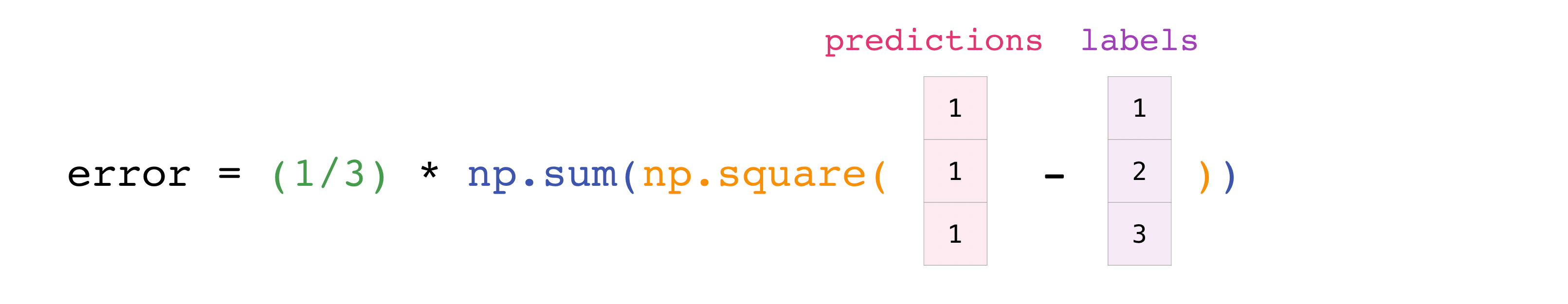
In this example, both the predictions and labels vectors contain three values,
meaning n has a value of three. After we carry out subtractions the values
in the vector are squared. Then NumPy sums the values, and your result is the
error value for that prediction and a score for the quality of the model.

How to save and load NumPy objects#
This section covers np.save, np.savez, np.savetxt,
np.load, np.loadtxt
You will, at some point, want to save your arrays to disk and load them back
without having to re-run the code. Fortunately, there are several ways to save
and load objects with NumPy. The ndarray objects can be saved to and loaded from
the disk files with loadtxt and savetxt functions that handle normal
text files, load and save functions that handle NumPy binary files with
a .npy file extension, and a savez function that handles NumPy files
with a .npz file extension.
The .npy and .npz files store data, shape, dtype, and other information
required to reconstruct the ndarray in a way that allows the array to be
correctly retrieved, even when the file is on another machine with different
architecture.
If you want to store a single ndarray object, store it as a .npy file using
np.save. If you want to store more than one ndarray object in a single file,
save it as a .npz file using np.savez. You can also save several arrays
into a single file in compressed npz format with savez_compressed.
It’s easy to save and load and array with np.save(). Just make sure to
specify the array you want to save and a file name. For example, if you create
this array:
>>> a = np.array([1, 2, 3, 4, 5, 6])
You can save it as “filename.npy” with:
>>> np.save('filename', a)
You can use np.load() to reconstruct your array.
>>> b = np.load('filename.npy')
If you want to check your array, you can run:
>>> print(b)
[1 2 3 4 5 6]
You can save a NumPy array as a plain text file like a .csv or .txt file
with np.savetxt.
For example, if you create this array:
>>> csv_arr = np.array([1, 2, 3, 4, 5, 6, 7, 8])
You can easily save it as a .csv file with the name “new_file.csv” like this:
>>> np.savetxt('new_file.csv', csv_arr)
You can quickly and easily load your saved text file using loadtxt():
>>> np.loadtxt('new_file.csv')
array([1., 2., 3., 4., 5., 6., 7., 8.])
The savetxt() and loadtxt() functions accept additional optional
parameters such as header, footer, and delimiter. While text files can be easier
for sharing, .npy and .npz files are smaller and faster to read. If you need more
sophisticated handling of your text file (for example, if you need to work with
lines that contain missing values), you will want to use the genfromtxt
function.
With savetxt, you can specify headers, footers, comments, and more.
Learn more about input and output routines here.
Importing and exporting a CSV#
It’s simple to read in a CSV that contains existing information. The best and
easiest way to do this is to use
Pandas.
>>> import pandas as pd

>>> # If all of your columns are the same type:
>>> x = pd.read_csv('music.csv', header=0).values
>>> print(x)
[['Billie Holiday' 'Jazz' 1300000 27000000]
 ['Jimmie Hendrix' 'Rock' 2700000 70000000]
 ['Miles Davis' 'Jazz' 1500000 48000000]
 ['SIA' 'Pop' 2000000 74000000]]

>>> # You can also simply select the columns you need:
>>> x = pd.read_csv('music.csv', usecols=['Artist', 'Plays']).values
>>> print(x)
[['Billie Holiday' 27000000]
 ['Jimmie Hendrix' 70000000]
 ['Miles Davis' 48000000]
 ['SIA' 74000000]]
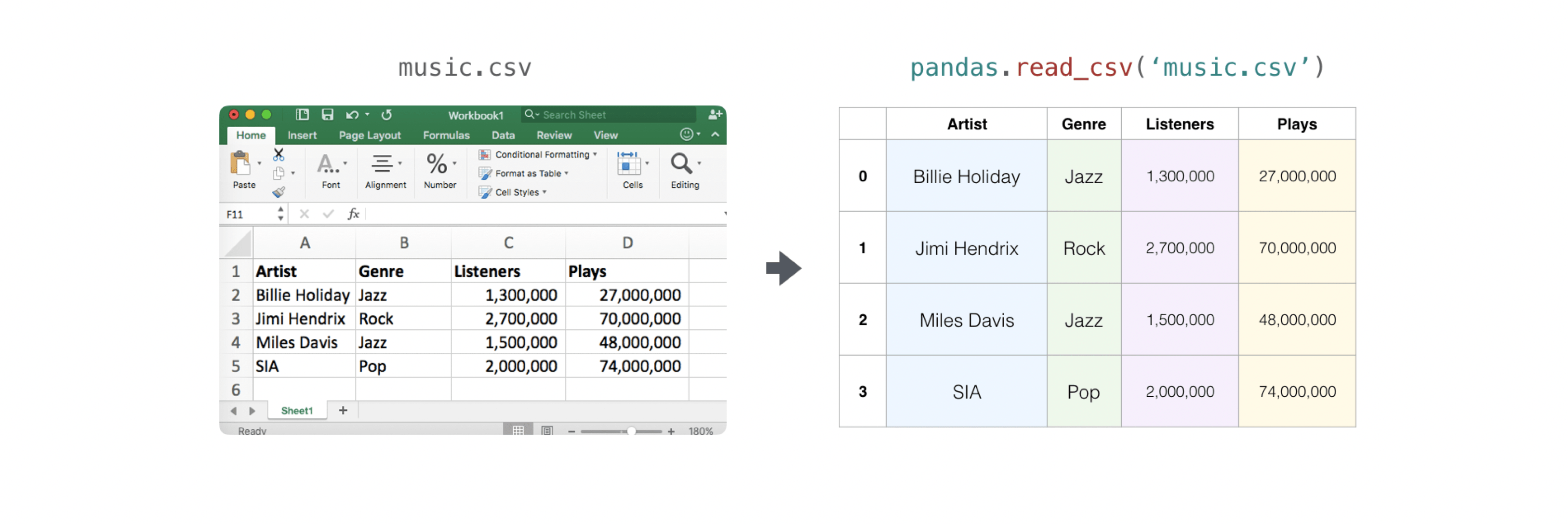
It’s simple to use Pandas in order to export your array as well. If you are new
to NumPy, you may want to create a Pandas dataframe from the values in your
array and then write the data frame to a CSV file with Pandas.
If you created this array “a”
>>> a = np.array([[-2.58289208,  0.43014843, -1.24082018, 1.59572603],
...               [ 0.99027828, 1.17150989,  0.94125714, -0.14692469],
...               [ 0.76989341,  0.81299683, -0.95068423, 0.11769564],
...               [ 0.20484034,  0.34784527,  1.96979195, 0.51992837]])
You could create a Pandas dataframe
>>> df = pd.DataFrame(a)
>>> print(df)
          0         1         2         3
0 -2.582892  0.430148 -1.240820  1.595726
1  0.990278  1.171510  0.941257 -0.146925
2  0.769893  0.812997 -0.950684  0.117696
3  0.204840  0.347845  1.969792  0.519928
You can easily save your dataframe with:
And read your CSV with:
>>> data = pd.read_csv('pd.csv')
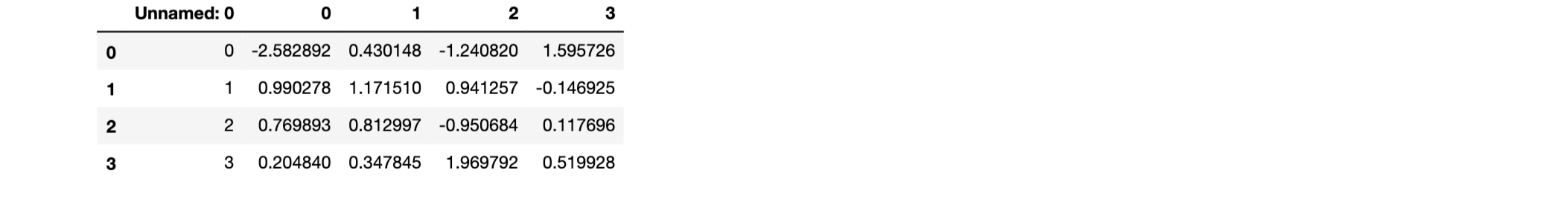
You can also save your array with the NumPy savetxt method.
>>> np.savetxt('np.csv', a, fmt='%.2f', delimiter=',', header='1, 2, 3, 4')
If you’re using the command line, you can read your saved CSV any time with a
command such as:
$ cat np.csv
#  1,  2,  3,  4
-2.58,0.43,-1.24,1.60
0.99,1.17,0.94,-0.15
0.77,0.81,-0.95,0.12
0.20,0.35,1.97,0.52
Or you can open the file any time with a text editor!
If you’re interested in learning more about Pandas, take a look at the
official Pandas documentation.
Learn how to install Pandas with the
official Pandas installation information.
Plotting arrays with Matplotlib#
If you need to generate a plot for your values, it’s very simple with
Matplotlib.
For example, you may have an array like this one:
>>> a = np.array([2, 1, 5, 7, 4, 6, 8, 14, 10, 9, 18, 20, 22])
If you already have Matplotlib installed, you can import it with:
>>> import matplotlib.pyplot as plt

# If you're using Jupyter Notebook, you may also want to run the following
# line of code to display your code in the notebook:

%matplotlib inline
All you need to do to plot your values is run:
>>> plt.plot(a)

# If you are running from a command line, you may need to do this:
# >>> plt.show()
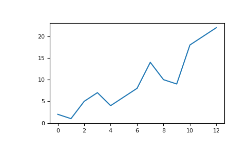
For example, you can plot a 1D array like this:
>>> x = np.linspace(0, 5, 20)
>>> y = np.linspace(0, 10, 20)
>>> plt.plot(x, y, 'purple') # line
>>> plt.plot(x, y, 'o')      # dots
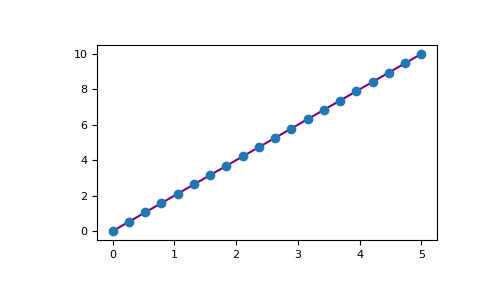
With Matplotlib, you have access to an enormous number of visualization options.
>>> fig = plt.figure()
>>> ax = fig.add_subplot(projection='3d')
>>> X = np.arange(-5, 5, 0.15)
>>> Y = np.arange(-5, 5, 0.15)
>>> X, Y = np.meshgrid(X, Y)
>>> R = np.sqrt(X**2 + Y**2)
>>> Z = np.sin(R)

>>> ax.plot_surface(X, Y, Z, rstride=1, cstride=1, cmap='viridis')
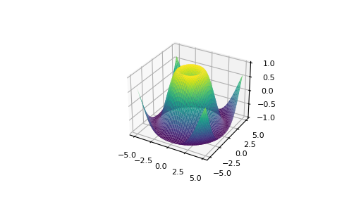
To read more about Matplotlib and what it can do, take a look at
the official documentation.
For directions regarding installing Matplotlib, see the official
installation section.
Image credits: Jay Alammar http://jalammar.github.io/
Время на прочтение
5 мин
Количество просмотров 357K
Предисловие переводчика
Доброго времени суток, Хабр. Запускаю цикл статей, которые являются переводом небольшого мана по numpy, ссылочка. Приятного чтения.
- Часть 2
- Часть 3
- Часть 4
Введение
NumPy это open-source модуль для python, который предоставляет общие математические и числовые операции в виде пре-скомпилированных, быстрых функций. Они объединяются в высокоуровневые пакеты. Они обеспечивают функционал, который можно сравнить с функционалом MatLab. NumPy (Numeric Python) предоставляет базовые методы для манипуляции с большими массивами и матрицами. SciPy (Scientific Python) расширяет функционал numpy огромной коллекцией полезных алгоритмов, таких как минимизация, преобразование Фурье, регрессия, и другие прикладные математические техники.
Установка
Если у вас есть Python(x, y) (Примечание переводчика: Python(x, y), это дистрибутив свободного научного и инженерного программного обеспечения для численных расчётов, анализа и визуализации данных на основе языка программирования Python и большого числа модулей (библиотек)) на платформе Windows, то вы готовы начинать. Если же нет, то после установки python, вам нужно установить пакеты самостоятельно, сначала NumPy потом SciPy. Установка доступна здесь. Следуйте установке на странице, там всё предельно понятно.
Немного дополнительной информации
Сообщество NumPy и SciPy поддерживает онлайн руководство, включающие гайды и туториалы, тут: docs.scipy.org/doc.
Импорт модуля numpy
Есть несколько путей импорта. Стандартный метод это — использовать простое выражение:
>>> import numpyТем не менее, для большого количества вызовов функций numpy, становится утомительно писать numpy.X снова и снова. Вместо этого намного легче сделать это так:
>>> import numpy as npЭто выражение позволяет нам получать доступ к numpy объектам используя np.X вместо numpy.X. Также можно импортировать numpy прямо в используемое пространство имен, чтобы вообще не использовать функции через точку, а вызывать их напрямую:
>>> from numpy import *Однако, этот вариант не приветствуется в программировании на python, так как убирает некоторые полезные структуры, которые модуль предоставляет. До конца этого туториала мы будем использовать второй вариант импорта (import numpy as np).
Массивы
Главной особенностью numpy является объект array. Массивы схожи со списками в python, исключая тот факт, что элементы массива должны иметь одинаковый тип данных, как float и int. С массивами можно проводить числовые операции с большим объемом информации в разы быстрее и, главное, намного эффективнее чем со списками.
Создание массива из списка:
a = np.array([1, 4, 5, 8], float)
>>> a
array([ 1.,  4.,  5.,  8.])
>>> type(a)
<class 'numpy.ndarray'>
Здесь функция array принимает два аргумента: список для конвертации в массив и тип для каждого элемента. Ко всем элементам можно получить доступ и манипулировать ими так же, как вы бы это делали с обычными списками:
>>> a[:2]
array([ 1.,  4.])
>>> a[3]
8.0
>>> a[0] = 5.
>>> a
array([ 5.,  4.,  5.,  8.])
Массивы могут быть и многомерными. В отличии от списков можно использовать запятые в скобках. Вот пример двумерного массива (матрица):
>>> a = np.array([[1, 2, 3], [4, 5, 6]], float)
>>> a
array([[ 1.,  2.,  3.],
[ 4.,  5.,  6.]])
>>> a[0,0]
1.0
>>> a[0,1]
2.0
Array slicing работает с многомерными массивами аналогично, как и с одномерными, применяя каждый срез, как фильтр для установленного измерения. Используйте «:» в измерении для указывания использования всех элементов этого измерения:
>>> a = np.array([[1, 2, 3], [4, 5, 6]], float)
>>> a[1,:]
array([ 4.,  5.,  6.])
>>> a[:,2]
array([ 3.,  6.])
>>> a[-1:, -2:]
array([[ 5.,  6.]])
Метод shape возвращает количество строк и столбцов в матрице:
>>> a.shape
(2, 3)
Метод dtype возвращает тип переменных, хранящихся в массиве:
>>> a.dtype
dtype('float64')
Тут float64, это числовой тип данных в numpy, который используется для хранения вещественных чисел двойной точности. Так же как float в Python.
Метод len возвращает длину первого измерения (оси):
a = np.array([[1, 2, 3], [4, 5, 6]], float)
>>> len(a)
2
Метод in используется для проверки на наличие элемента в массиве:
>>> a = np.array([[1, 2, 3], [4, 5, 6]], float)
>>> 2 in a
True
>>> 0 in a
False
Массивы можно переформировать при помощи метода, который задает новый многомерный массив. Следуя следующему примеру, мы переформатируем одномерный массив из десяти элементов во двумерный массив, состоящий из пяти строк и двух столбцов:
>>> a = np.array(range(10), float)
>>> a
array([ 0.,  1.,  2., 3.,  4.,  5.,  6.,  7.,  8.,  9.])
>>> a = a.reshape((5, 2))
>>> a
array([[ 0.,  1.],
[ 2.,  3.],
[ 4.,  5.],
[ 6.,  7.],
[ 8.,  9.]])
>>> a.shape
(5, 2)
Обратите внимание, метод reshape создает новый массив, а не модифицирует оригинальный.
Имейте ввиду, связывание имен в python работает и с массивами. Метод copy используется для создания копии существующего массива в памяти:
>>> a = np.array([1, 2, 3], float)
>>> b = a
>>> c =  a.copy()
>>> a[0] = 0
>>> a
array([0., 2., 3.])
>>> b
array([0., 2., 3.])
>>> c
array([1., 2., 3.])
Списки можно тоже создавать с массивов:
>>> a = np.array([1, 2, 3], float)
>>> a.tolist()
[1.0, 2.0, 3.0]
>>> list(a)
[1.0, 2.0, 3.0]
Можно также переконвертировать массив в бинарную строку (то есть, не human-readable форму). Используйте метод tostring для этого. Метод fromstring работает в для обратного преобразования. Эти операции иногда полезны для сохранения большого количества данных в файлах, которые могут быть считаны в будущем.
>>> a = array([1, 2, 3], float)
>>> s = a.tostring()
>>> s
'x00x00x00x00x00x00xf0?x00x00x00x00x00x00x00@x00x00x00x00x00x00x08@'
>>> np.fromstring(s)
array([ 1.,  2.,  3.])
Заполнение массива одинаковым значением.
>>> a = array([1, 2, 3], float)
>>> a
array([ 1.,  2.,  3.])
>>> a.fill(0)
>>> a
array([ 0.,  0.,  0.])
Транспонирование массивов также возможно, при этом создается новый массив:
>>> a = np.array(range(6), float).reshape((2, 3))
>>> a
array([[ 0.,  1.,  2.],
[ 3.,  4.,  5.]])
>>> a.transpose()
array([[ 0.,  3.],
[ 1.,  4.],
[ 2.,  5.]])
Многомерный массив можно переконвертировать в одномерный при помощи метода flatten:
>>> a = np.array([[1, 2, 3], [4, 5, 6]], float)
>>> a
array([[ 1.,  2.,  3.],
[ 4.,  5.,  6.]])
>>> a.flatten()
array([ 1.,  2.,  3.,  4.,  5.,  6.])
Два или больше массивов можно сконкатенировать при помощи метода concatenate:
>>> a = np.array([1,2], float)
>>> b = np.array([3,4,5,6], float)
>>> c = np.array([7,8,9], float)
>>> np.concatenate((a, b, c))
array([1., 2., 3., 4., 5., 6., 7., 8., 9.])
Если массив не одномерный, можно задать ось, по которой будет происходить соединение. По умолчанию (не задавая значения оси), соединение будет происходить по первому измерению:
>>> a = np.array([[1, 2], [3, 4]], float)
>>> b = np.array([[5, 6], [7,8]], float)
>>> np.concatenate((a,b))
array([[ 1.,  2.],
[ 3.,  4.],
[ 5.,  6.],
[ 7.,  8.]])
>>> np.concatenate((a,b), axis=0)
array([[ 1.,  2.],
[ 3.,  4.],
[ 5.,  6.],
[ 7.,  8.]])
>>>
np.concatenate((a,b), axis=1)
array([[ 1.,  2.,  5.,  6.],
[ 3.,  4.,  7.,  8.]])
В заключении, размерность массива может быть увеличена при использовании константы newaxis в квадратных скобках:
>>> a = np.array([1, 2, 3], float)
>>> a
array([1., 2., 3.])
>>> a[:,np.newaxis]
array([[ 1.],
[ 2.],
[ 3.]])
>>> a[:,np.newaxis].shape
(3,1)
>>> b[np.newaxis,:]
array([[ 1.,  2.,  3.]])
>>> b[np.newaxis,:].shape
(1,3)
Заметьте, тут каждый массив двумерный; созданный при помощи newaxis имеет размерность один. Метод newaxis подходит для удобного создания надлежаще-мерных массивов в векторной и матричной математике.
На этом у нас конец первой части перевода. Спасибо за внимание.
#статьи
- 28 окт 2022
-

0
Подробный гайд по самому популярному Python-инструменту для анализа данных и обучения нейронных сетей.
Иллюстрация: A Wolker / Pexels / Colowgee для Skillbox Media

Любитель научной фантастики и технологического прогресса. Хорошо сочетает в себе заумного технаря и утончённого гуманитария. Пишет про IT и радуется этому.
NumPy — это открытая бесплатная Python-библиотека для работы с многомерными массивами, этакий питонячий аналог Matlab. NumPy чаще всего используют в анализе данных и обучении нейронных сетей — в каждой из этих областей нужно проводить много вычислений с такими матрицами.
В этой статье мы собрали всё необходимое для старта работы с этой библиотекой — вам хватит получаса, чтобы разобраться в основных возможностях.
- Базовые функции
- Доступ к элементам
- Создание специальных массивов
- Математические операции
- Копирование и организации
- Дополнительные возможности
Что запомнить
NumPy не просто работает с многомерными массивами, но и делает это быстро. Вообще, интерпретируемые языки производят вычисления медленнее компилируемых, а Python как раз язык интерпретируемый. NumPy же сделана так, чтобы эффективно работать с наборами чисел любого размера в Python.
Библиотека частично написана на Python, а частично на C и C++ — в тех местах, которые требуют скорости. Кроме того, код NumPy оптимизирован под большинство современных процессоров. Кстати, как и у Matlab, для NumPy существуют пакеты, расширяющие её функциональность, — например, библиотека SciPy или Matplotlib.
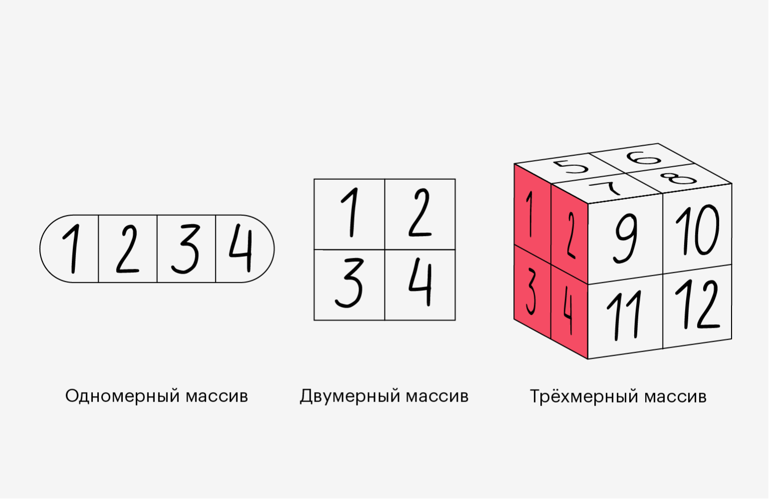
Инфографика: Оля Ежак для Skillbox Media
Массивы в NumPy отличаются от обычных списков и кортежей в Python тем, что они должны состоять только из элементов одного типа. Такое ограничение позволяет увеличить скорость вычислений в 50 раз, а также избежать ненужных ошибок с приведением и обработкой типов.
Мы установим NumPy через платформу Anaconda, которая содержит много разных библиотек для Python. А ещё покажем, как это сделать через PIP.
NumPy можно также использовать через Jupyter Notebook, Google Colab или другими средствами — как вам удобнее. Поэтому выбирайте любой способ и пойдёмте изучать его.
Сначала надо зайти на официальный сайт Anaconda, чтобы скачать последнюю версию Python и NumPy: есть готовые пакеты под macOS, Windows и Linux.

Скриншот: Skillbox Media
Затем открываем установщик, соглашаемся со всеми пунктами и выбираем место для установки.

Скриншот: Skillbox Media
Чтобы убедиться, что Python точно установился, открываем консоль и вводим туда команду python3 — должен запуститься интерпретатор Python, в котором можно писать код. Выглядит всё это примерно так:
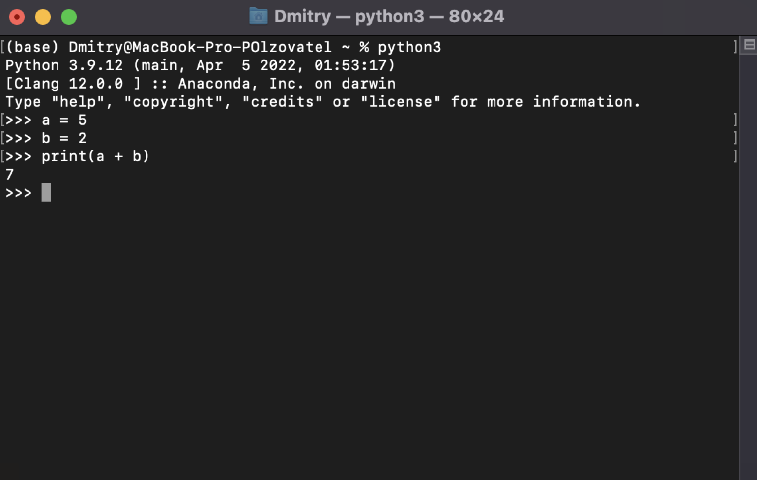
Скриншот: Skillbox Media
Anaconda уже содержит в себе много полезностей — например, NumPy, SciPy, Pandas. Поэтому больше ничего устанавливать не нужно. Достаточно проверить, что библиотека NumPy действительно работает. Введите в интерпретаторе Python в консоли такие команды — пока не важно, что это и как работает, об этом поговорим ниже.
import numpy as np
Следом вот это:
a = np.array ([1,2,3])
А потом выводим значение переменной a — чтобы убедиться, что всё работает:
print (a)
Должно получиться что-то вроде вывода на скриншоте:
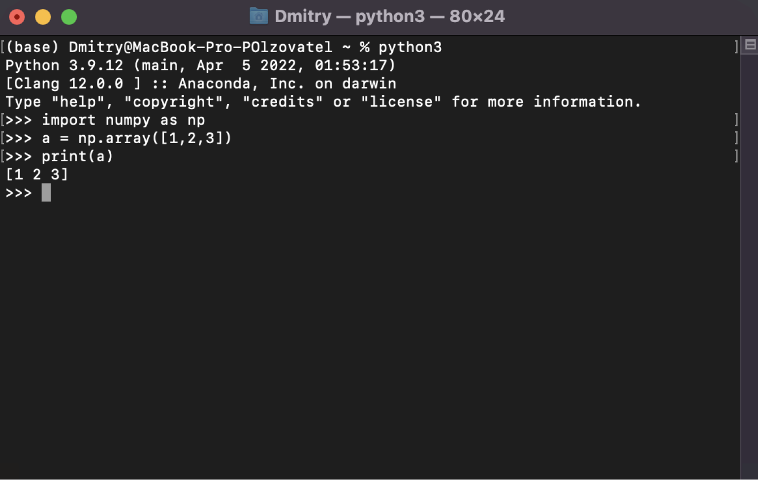
Скриншот: Skillbox Media
Если вам не хочется скачивать огромный пакет Anaconda, вы можете установить только NumPy с помощью встроенного питоновского менеджера пакетов PIP.
Для этого сначала нужно установить Python с официального сайта. Заходим на него, переходим во вкладку Downloads и видим справа последнюю актуальную версию Python:

Скриншот: Skillbox Media
После этого начинается стандартная процедура: выбираем место установки и соглашаемся со всеми пунктами.

В конце нас должны поздравить.

Скриншот: Skillbox Media
Теперь нужно скачать библиотеку NumPy. Открываем консоль и вводим туда команду pip install numpy.
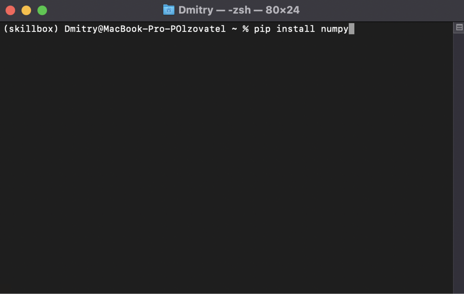
Скриншот: Skillbox Media
Если вдруг у вас выпала ошибка, значит, нужно написать другую похожую команду — pip3 install numpy.
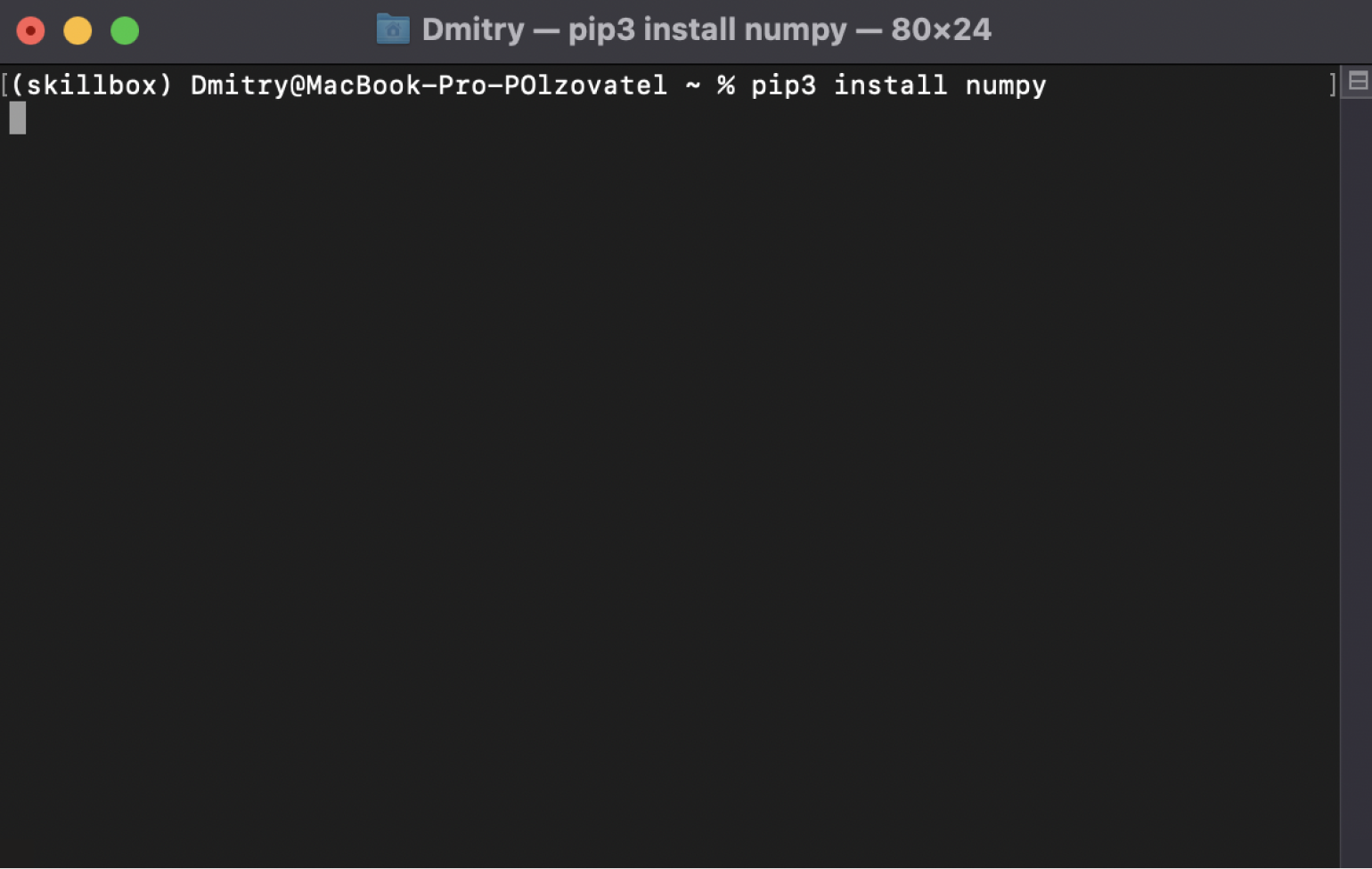
Скриншот: Skillbox Media
Теперь у нас точно должна установиться NumPy. Правда, тут нас уже никто не поздравляет — лишь сухо отмечают, что установка завершилась успешно.
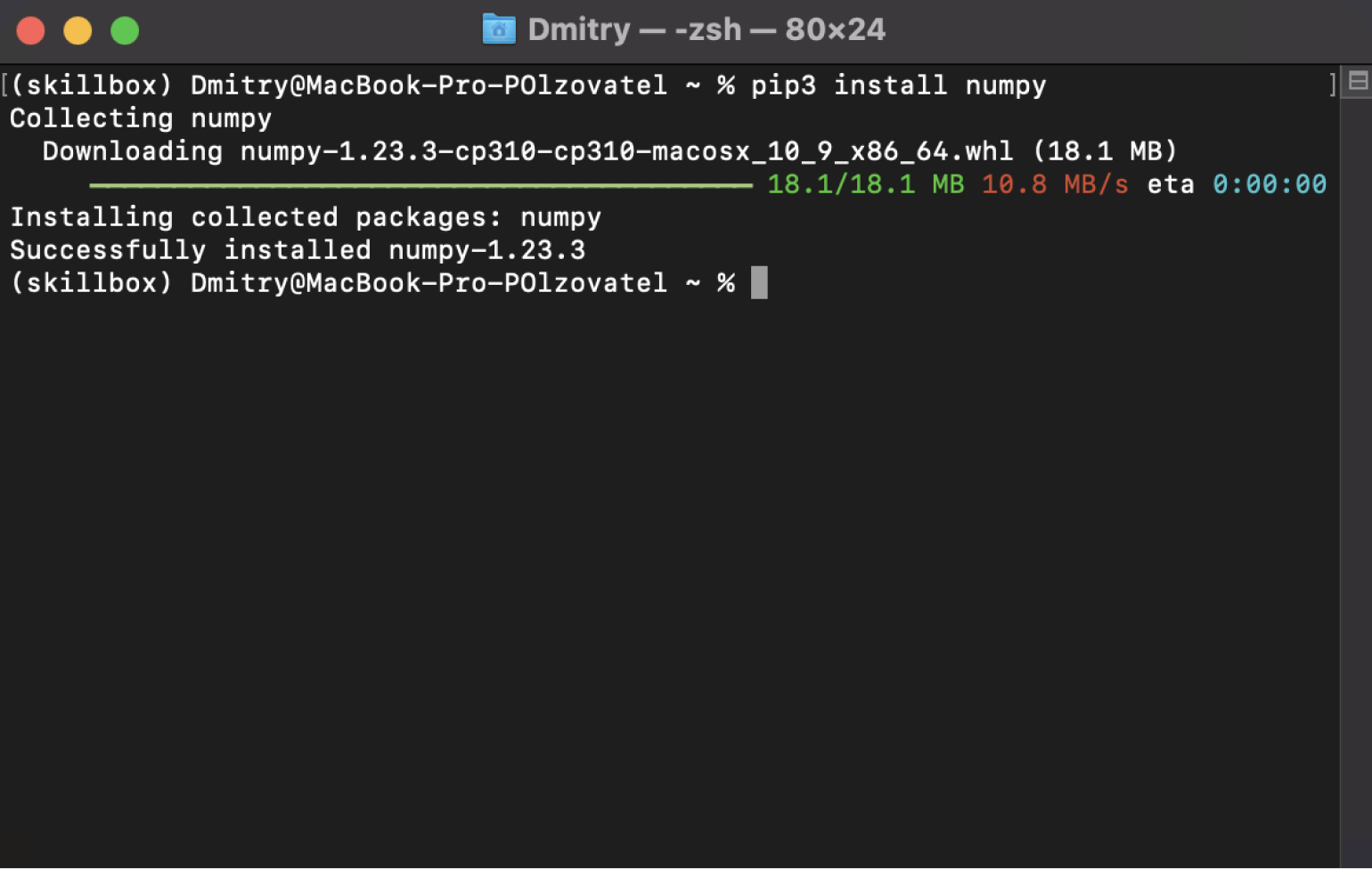
Скриншот: Skillbox Media
Перед тем как использовать NumPy, нужно подключить библиотеку в Python-коде — а вы думали, достаточно установить его? Нет, Python ещё должен узнать, что конкретно в этом проекте NumPy нам нужен.
import numpy as np
np — это уже привычное сокращение для NumPy в Python-сообществе. Оно позволяет быстро обращаться к методам библиотеки (две буквы проще, чем пять). Мы тоже будем придерживаться этого сокращения — мы же профессионалы! Хотя можно использовать NumPy и без присваивания отдельного сокращения или назвать её любыми приятными для вас буквами и символами. Но всё же рекомендуем следовать традициям сообщества, чтобы избежать недопонимания со стороны других программистов.
Теперь приступим к изучению базовых понятий и функций NumPy. А чтобы лучше усвоить изученный материал, рекомендуем внимательно изучать код, самостоятельно переписывать его и поиграться с параметрами и числами.
Главный объект библиотеки NumPy — массив. Создаётся он очень просто:
a = np.array([1, 2, 3])
Мы объявили переменную a и использовали встроенную функцию array. В неё нужно положить сам Python-список, который мы хотим создать. Он может быть любой формы: одномерный, двумерный, трёхмерный и так далее. Выше мы создали одномерный массив. Давайте создадим и другие:
a2 = np.array([[1, 2, 3], [4, 5, 6]])
a3 = np.array([[[1, 2, 3], [4, 5, 6]], [[7, 8, 9], [10, 11, 12]]])
Получилось огромное количество скобок. Чтобы понять, как всё это выглядит, воспользуемся функцией print:
print(a)
[1 2 3]

print(a2)
[[1 2 3]
 [4 5 6]]

print(a3)
[[[1 2 3]
  [4 5 6]]

 [[7 8 9]
  [10 11 12]]]
Как мы видим, в первом случае получился двумерный массив, который состоит из двух одномерных. А во втором — трёхмерный, состоящий из двумерных. Если двигаться вверх по измерениям, то они будут следовать похожей логике:
- четырёхмерный массив состоит из трёхмерных;
- пятимерный массив — это несколько четырёхмерных;
- n-мерный массив — это несколько (n-1)-мерных.
Проще показать это на иллюстрации (главное, не потеряйтесь в измерениях):
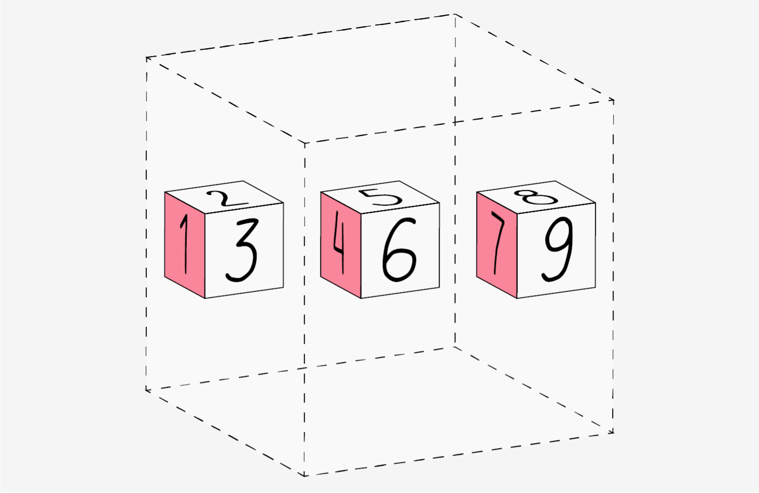
Инфографика: Оля Ежак для Skillbox Media
В NumPy-массивы можно передавать не только целые числа, но и дробные:
b = np.array([1.4, 2.5, 3.7])

print(b)
[1.4 2.5 3.7]
А если вы хотите указать конкретный тип, то это можно сделать с помощью дополнительного параметра dtype:
c = np.array([1, 2, 3], dtype='float32')

print(c)
[1. 2. 3.]
Целые числа сразу были приведены к числам с плавающей точкой. Таких преобразований существует много — они нужны, чтобы не занимать лишнюю память. Например, числа int32 занимают 32 бита, или 4 байта, а int16 — 16 бит, или 2 байта. Программисты используют параметр dtype, когда точно знают, что их переменные будут находиться в диапазоне от −32 768 до 32 767.
Если реальные значения элементов массива выйдут за рамки явно указанного типа, то их значения в какой-то момент просто обнулятся и начнут отсчёт заново:
# Допустим, a — это переменная типа int16, у которой максимальное значение — 32 767

a = 32 000

b = 768
print(a + b)
-32768
Как мы видим, результат обнулился до своего минимального значения — –32 768.
Теперь, когда мы умеем создавать массивы и задавать им разные значения, давайте узнаем, какие у них есть встроенные функции.
Допустим, у нас есть такой объект:
a = np.array([1,2,3], dtype='int32')

print(a)
[1 2 3]
Чтобы узнать, сколько у него измерений, воспользуемся функцией ndim:
print(a.ndim)
1
Всё верно, ведь у нас одномерный массив, или вектор. Если бы он был двумерным, то и результат оказался бы другим:
b = np.array([[1, 2, 3], [4, 5, 6]])

print(b.ndim)
2
Хорошо, с размерностью понятно. А как посчитать количество строк и столбцов? Для этого есть функция shape:
print(a.shape)
(3, )
Получилось слегка странно, но всему есть объяснение. Дело в том, что вектор — это всего лишь одномерный массив. У векторов в библиотеке NumPy есть только строки — или элементы. Поэтому функция shape выдала число 3.
С двумерными массивами ситуация понятнее:
print(b.shape)
(2, 3)
В b — 2 строки и 3 столбца.
Для трёхмерных и n-мерных массивов функция shape будет добавлять дополнительные цифры в кортеже через запятую:
с = np.array([[[1, 2, 3], [4, 5, 6]], [[7, 8, 9], [10, 11, 12]]])

print(c.shape)
(2, 2, 3)
Читается это так: в объекте c два трёхмерных массива с двумя строками и тремя столбцами.
Кроме размерностей, можно также узнать тип элементов — в этом поможет функция dtype (не путайте её с одноимённым параметром):
a = np.array([1,2,3], dtype='int32')

print(a.dtype)
dtype('int32')
Если не присваивать тип элементам вручную, по умолчанию будет задан int32.
Ещё можно узнать количество элементов с помощью функции size:
print(a.size)
3
А через функции itemsize и nbytes можно узнать, какое количество байт в памяти занимает один элемент и какое количество байт занимает весь массив:
b = np.array([[1, 2, 3], [4, 5, 6]], dtype='int16')

print(b.itemsize)
2

print(b.nbytes)
12
Один элемент занимает 2 байта, а весь объект b из 6 элементов — 2 × 6 = 12 байтов.
В NumPy можно обращаться к отдельным элементам, строкам или столбцам, а также точечно выбирать последовательность нужных элементов. Рассмотрим всё подробнее.
Допустим, у нас есть двумерный массив:
a = np.array([[1, 2, 3, 4, 5, 6, 7], [8, 9, 10, 11, 12, 13, 14]])

print(a)
[[ 1  2  3  4  5  6  7]
 [ 8  9 10 11 12 13 14]]
И мы хотим достать их него элемент, который находится в первой строке на пятом месте. Сделать это можно с помощью специального оператора []:
print(a[0, 4])
5
Почему 0 и 4? Потому что нумерация элементов в Python начинается с нуля, а значит, первая строка будет нулевой, а пятый столбец — четвёртым.
Если бы у нас был трёхмерный массив, обращение к его элементам было бы похожим:
c = np.array([[[1, 2, 3], [4, 5, 6]], [[7, 8, 9], [10, 11, 12]]])

print(c)
[[[ 1  2  3]
  [ 4  5  6]]

 [[ 7  8  9]
  [10 11 12]]]

print(c[1, 1, 1])
11
Здесь мы сначала обратились ко второму двумерному массиву, а затем выбрали в нём вторую строку и второй столбец. Там и находилось число 11.
Кроме отдельных элементов, в библиотеке NumPy можно обратиться к целой строке или столбцу с помощью оператора :. Он позволяет выбрать все элементы указанной строки или столбца:
print(a[0, :])
[1 2 3 4 5 6 7]

print(a[:, 0])
[1 8]
В первом случае мы выбрали всю первую строку, а во втором — первый столбец.
Ещё можно использовать продвинутые способы выделения нужных нам элементов.
Кстати, оператор : на самом деле представляет собой сокращённую форму конструкции начальный_индекс: конечный_индекс: шаг.
Давайте остановимся на ней подробнее:
b = np.array([[1, 2, 3, 4], [5, 6, 7, 8]])

print(b[0, 1:4:2])
[2 4]
Мы указали, что хотим выбрать первую строку, а затем уточнили, какие именно столбцы нам нужны: 1:4:2.
- Первое число означает, что мы начинаем брать элементы с первого индекса — второго столбца.
- Второе число — что мы заканчиваем итерацию на четвёртом индексе, то есть проходим всю строку.
- Третье число указывает, с каким шагом мы идём по строке. В нашем примере — с шагом в два элемента. То есть мы пройдём по элементам 1, 3 и 5.
Давайте посмотрим на другой пример:
a = np.array([[1, 2, 3, 4, 5, 6, 7], [8, 9, 10, 11, 12, 13, 14]])

print(a)
[[ 1  2  3  4  5  6  7]
 [ 8  9 10 11 12 13 14]]

print(a[1, 0:-1:3])
[8, 11]
Здесь мы использовали отрицательные индексы — они позволяют считать индексы элементов справа налево. –1 означает, что последний индекс — это последний столбец второй строки. Заметьте, что 6-й столбец не вывелся. Это значит, что NumPy не доходит до этого индекса, а заканчивает обход на один индекс раньше.
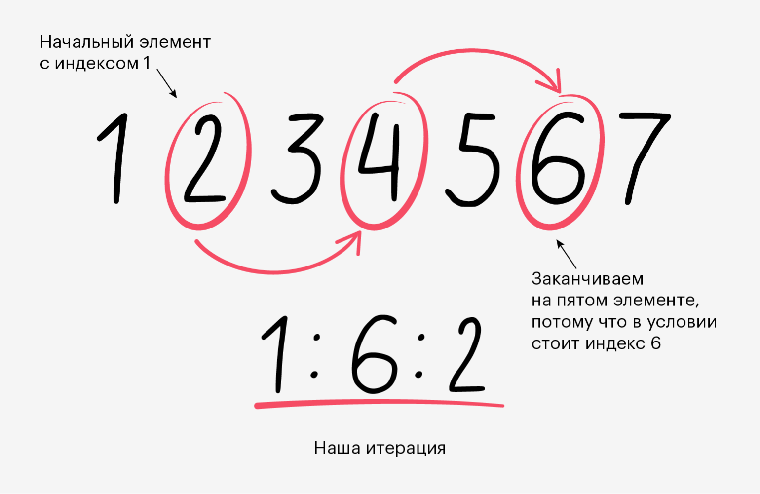
Инфографика: Оля Ежак для Skillbox Media
Ещё мы можем менять значения в NumPy-массиве с помощью той же операции доступа к элементам. Например:
c = np.array([[0, 2], [4, 6]])
c[0, 0] = 1

print(c)
[[1 2]
 [4 6]]
Мы заменили элемент из первой строки и первого столбца (элемент 0) на единицу. И наш массив успешно изменился.
Кроме отдельных элементов, можно заменять любые последовательности элементов с помощью конструкции начальный_индекс: конечный_индекс: шаг и её упрощённой версии — :.
c = np.array([[0, 2], [4, 6]]) с[0, :] = [3, 3] print(c) [[3 3] [4 6]]
Теперь в с вся первая строка заменилась на тройки. Главное при такой замене — учитывать размер строки, чтобы не возникло ошибок. Например, если присвоить первой строке вектор из трёх элементов, интерпретатор будет ругаться:
c = np.array([[0, 2], [4, 6]]) c[0, :] = [3, 3, 3] Traceback (most recent call last): File "<stdin>", line 1, in <module> ValueError: could not broadcast input array from shape (3,) into shape (2,)
Текст ошибки сообщает, что нельзя присвоить одномерному массиву с размером 2 массив размером 3.
Мы научились создавать массивы любой размерности. Но иногда хочется создать их с уже заполненными значениями — например, забить все ячейки нулями или единицами. NumPy может и это.
Массив из нулей. Чтобы создать его, используем функцию zeros.
a = np.zeros((2, 2)) print(a) [[0. 0.] [0. 0.]]
Первое, что нужно помнить, — как задавать размер. Он задаётся кортежем (2, 2). Если указать размер без скобок, то снова получим ошибку:
a = np.zeros(2, 2) Traceback (most recent call last): File "<stdin>", line 1, in <module> TypeError: Cannot interpret '2' as a data type
А всё потому, что без скобок NumPy расценивает второй элемент (число 2) как тип данных, который должен быть указан для параметра dtype.
Если указать только одно число, создастся вектор размером два элемента. В этом случае уже не нужно ставить дополнительные скобки:
a = np.zeros(2) print(a) [0. 0.]
Ещё стоит отметить, что элементам по умолчанию присваивается тип float64. Это дробные числа, которые занимают в памяти 64 бита, или 8 байт. Если нужны именно целые числа, то мы по старой схеме указываем это в параметре dtype — через запятую:
a = np.zeros(2, dtype='int32') print(a) [0 0]
Массив из единиц. Он создаётся точно так же, как и из нулей, но используется функция ones:
b = np.ones((4, 2, 2), dtype='int32') print(b) [[[1 1] [1 1]] [[1 1] [1 1]] [[1 1] [1 1]] [[1 1] [1 1]]]
Здесь мы создали трёхмерный массив из четырёх двумерных, каждый из которых имеет две строки и два столбца. А также указали, что элементы должны иметь тип int32.
Массив из произвольных чисел. Иногда бывает нужно заполнить массив какими-то отличными от нуля и единицы числами. В этом поможет функция full:
c = np.full((2, 2), 5) print(c) [[5 5] [5 5]]
Здесь мы сначала указали, какой размер должен быть у массива через кортеж, — (2,2), а затем число, которым мы хотим заполнить все его элементы, — 5.
Равно как и у функций zeros и ones, элементы по умолчанию будут иметь тип float64. А размер должен передаваться в виде кортежа — (2, 2).
Массив случайных чисел. Он создаётся с помощью функции random.rand:
d = np.random.rand(3, 2) print(d) [[0.76088962 0.14281283] [0.32124888 0.34894434] [0.66903093 0.72899792]]
Получилось что-то странное. Но так и должно быть — ведь NumPy генерирует случайные числа в диапазоне от 0 до 1 с восемью знаками после запятой.
Ещё одна странность — то, как задаётся размер. Здесь это нужно делать не через кортеж (3, 2), а просто указывая размерности через запятую. Всё потому, что в функции random.rand нет параметра dtype.
Чтобы создать массив случайных чисел, нужно воспользоваться функцией random.randint:
e = np.random.randint(-5, 10, size=(4, 4)) print(e) [[ 3 1 -4 3] [ 0 -2 5 3] [ 5 -1 9 2] [ 0 -4 9 -2]]
У нас получился массив размером четыре на четыре — size=(4, 4) — с целыми числами из диапазона от –5 до 10. Как и в предыдущем случае, создаётся такой массив слегка странно — но такова жизнь NumPy-программистов.
Единичная матрица. Она нужна тем, кто занимается линейной алгеброй. По диагонали такой матрицы элементы равны единице, а все остальные элементы — нулю. Создаётся она с помощью функции identity или eye:
i = np.identity(4) print(i) [[1. 0. 0. 0.] [0. 1. 0. 0.] [0. 0. 1. 0.] [0. 0. 0. 1.]]
Здесь задаётся только количество строк матрицы, потому что единичная матрица должна быть симметричной — иметь одинаковое количество строк и столбцов.
И всё также можно указать тип элементов с помощью параметра dtype:
i = np.identity(4, dtype='int32') print(i) [[1 0 0 0] [0 1 0 0] [0 0 1 0] [0 0 0 1]]
Массивы из NumPy поддерживают все стандартные арифметические операции — например, сложение, деление, вычитание. Работает это поэлементно:
a = np.array([1, 2, 3, 4]) print(a) [1 2 3 4] print(a + 3) [4 5 6 7]
К каждому элементу a прибавилось число 3, а размерность не изменилась. Все остальные операции работают точно так же:
print(a - 2) [-1 0 1 2] print(a * 2) [2 4 6 8] print(a / 2) [0.5 1. 1.5 2.] #Здесь тип элементов приведён к 'float64' print(a ** 2) [1 4 9 16]
Ещё можно проводить любые математические операции с массивами одинакового размера:
a = np.array([[1, 2], [3, 4]]) b = np.array([[2, 2], [2, 2]]) print(a + b) [[3 4] [5 6]] print(a * b) [[2 4] [6 8]] print(a ** b) [[ 1 4] [ 9 16]]
Здесь каждый элемент a складывается, умножается и возводится в степень на элемент из такой же позиции массива b.
Кроме примитивных операций, в NumPy можно проводить и более сложные — например, вычислить косинус:
a = np.array([[1, 2], [3, 4]]) print(np.cos(a)) [[ 0.54030231 -0.41614684] [-0.9899925 -0.65364362]]
Все математические функции вызываются по похожему шаблону: сначала пишем np.название_математической_функции, а потом передаём внутрь массив — как мы и сделали выше.
Ещё к массивам можно применять различные операции из линейной алгебры, математической статистики и так далее. Давайте для примера перемножим матрицы по правилам линейной алгебры:
a = np.ones((2, 3)) print(a) [[1. 1. 1.] [1. 1. 1.]] b = np.full((3, 2), 2) print(b) [[2 2] [2 2] [2 2]] print(np.matmul(a, b)) [[6. 6.] [6. 6.]]
Не будем разбирать математическую составляющую — предполагается, что вы уже знакомы с математикой и используете NumPy для выражения операций языком программирования. Полный список всех поддерживаемых в библиотеке операций можно найти в официальной документации.
Если в NumPy вы присвоите массив другой переменной, то просто создадите ссылку на него. Разберём на примере:
a = np.array([1, 2, 3]) b = a b[0] = 5 print(b) [5 2 3] print(a) [5 2 3]
Как мы видим, при изменении b меняется также и a. Дело в том, что массивы в NumPy — это только ссылки на области в памяти. Поэтому, когда мы присвоили a переменной b, на самом деле мы просто присвоили ей ссылку на первый элемент a в памяти.
Чтобы создать независимую копию a, используйте функцию copy:
a = np.array([1, 2, 3]) b = a.copy() b[0] = 5 print(b) [5 2 3] print(a) [1 2 3]
Ещё мы можем менять размер массива с помощью функции reshape:
a = np.array([[1, 2, 3, 4], [5, 6, 7, 8]]) print(a) [[1 2 3 4] [5 6 7 8]] b = a.reshape((4, 2)) print(b) [[1 2] [3 4] [5 6] [7 8]]
Изначально размер a был 2 на 4. Мы переделали его под 4 на 2. Заметьте: новые размеры должны соответствовать количеству элементов. В противном случае Python вернет ошибку:
a = np.array([[1, 2, 3, 4], [5, 6, 7, 8]]) b = a.reshape((4, 3)) Traceback (most recent call last): File "<stdin>", line 1, in <module> ValueError: cannot reshape array of size 8 into shape (4,3)
Ещё NumPy позволяет нам «наслаивать» массивы друг на друга и соединять их с помощью функций vstack и hstack:
v1 = np.array([1, 2, 3]) v2 = np.array([9, 8, 7]) v3 = np.vstack([v1, v2]) print(v3) [[1 2 3] [9 8 7]]
Здесь мы создали двумерный массив из двух векторов одинакового размера, которые «поставили» друг на друга. То же самое можно сделать и горизонтально:
h1 = np.ones((2, 4)) h2 = np.zeros((2, 2)) h3 = np.hstack((h1, h2)) print(h3) [[1. 1. 1. 1. 0. 0.] [1. 1. 1. 1. 0. 0.]]
К массиву из единиц справа присоединился массив из нулей. Главное — чтобы количество строк в обоих было одинаковым, иначе вылезет ошибка:
h1 = np.ones((2, 4)) h2 = np.zeros((3, 2)) h3 = np.hstack((h1, h2)) Traceback (most recent call last): File "<stdin>", line 1, in <module> File "<__array_function__ internals>", line 5, in hstack File "/Users/Dmitry/opt/anaconda3/lib/python3.9/site-packages/numpy/core/shape_base.py", line 345, in hstack return _nx.concatenate(arrs, 1) File "<__array_function__ internals>", line 5, in concatenate ValueError: all the input array dimensions for the concatenation axis must match exactly, but along dimension 0, the array at index 0 has size 2 and the array at index 1 has size 3
Эта ошибка говорит, что количество строк не совпадает.
NumPy поддерживает другие полезные функции, которые используются реже, но знать о которых полезно. Например, одна из таких функций — чтение файлов с жёсткого диска.
Чтение данных из файла. Допустим, у нас есть файл data.txt с таким содержимым:
1,2,3,5,6,7 8,1,4,2,6,4 9,0,1,7,3,4
Мы можем записать числа в NumPy-массив с помощью функции genfromtxt:
filedata = np.genfromtxt('data.txt', delimiter=',') filedata = filedata.astype('int32') print(filedata) [[1 2 3 5 6 7] [8 1 4 2 6 4] [9 0 1 7 3 4]]
Сначала мы достали данные из файла data.txt через функцию genfromtxt. В ней нужно указать считываемый файл, а затем разделитель — чтобы NumPy понимал, где начинаются и заканчиваются числа. У нас разделителем будет ,.
Затем нам нужно привести числа к формату int32 с помощью функции astype, передав в неё нужный нам тип.
Булевы выражения. Ещё одна из возможностей NumPy — булевы выражения для элементов массива. Они позволяют узнать, какие элементы отвечают определённым условиям — например, больше ли каждое число массива 50.
Допустим, у нас есть массив a и мы хотим проверить, действительно ли все его элементы больше 5:
a = np.array([[1, 5, 8], [3, 4, 2]]) print(a > 5) [[False False True] [False False False]]
На выходе — массив с «ответом» для каждого элемента: больше ли он числа 5. Если меньше или равно, то стоит False, иначе — True.
С помощью булевых выражений можно составлять и более сложные конструкции — например, создавать новые массивы из элементов, которые отвечают определённым условиям:
a = np.array([[1, 5, 8], [3, 4, 2], [2, 6, 7]]) print(a[a > 3]) [5 8 4 6 7]
Мы получили вектор, состоящий из элементов массива a, которые больше трёх.
- NumPy — это библиотека для эффективной работы с массивами любого размера. Она достигает высокой производительности, потому что написана частично на C и C++ и в ней соблюдается принцип локальности — она хранит все элементы последовательно в одном месте.
- Перед тем как использовать NumPy в коде, его нужно подключить с помощью команды import numpy as np.
- Основа NumPy — массив. Чтобы его создать, нужно использовать функцию array и передать туда список в качестве первого аргумента. Вторым аргументом через dtype можно указать тип для всех элементов — например, int16 или float32. По умолчанию для целых чисел указывается int32, а для десятичных — float64.
- Функция ndim позволяет узнать, сколько измерений у массива; shape — его структуру (сколько столбцов и строк); dtype — какой тип у элементов; size — количество элементов; itemsize — сколько байтов занимает один элемент; nbytes — сколько всего памяти занимает массив.
- К элементам массива можно обращаться с помощью оператора [], где указываются индексы нужного элемента. Важно помнить, что индексация начинается с нуля. А ещё в NumPy можно выбирать сразу целые строки или столбцы с помощью оператора : и его продвинутой версии — начальный_индекс: конечный_индекс: шаг.
- Функции zeros, ones, full, random.rand, random.randint, identity и eye помогают быстро создать массивы любого размера с заполненными элементами.
- Все арифметические операции, которые доступны в Python, применимы и к массивам NumPy. Главное — помнить, что операции проводятся поэлементно. А для сложных операций, таких как вычисление производной, также есть свои функции.
- NumPy-массивы нельзя просто присвоить другой переменной, чтобы скопировать. Для этого существует функция copy. А чтобы поменять структуру данных, можно применить функции reshape, vstack и hstack.
- Ещё в NumPy есть дополнительные функции — например, чтение из файла с помощью genfromtxt и булевы выражения, которые позволяют выбирать элементы из набора данных по заданным условиям.

Научитесь: Профессия Data Scientist
Узнать больше
Предок NumPy, Numeric, был разработан Джимом Хугунином. Также был создан пакет Numarray с дополнительной функциональностью. В 2005 году Трэвис Олифант выпустил пакет NumPy, добавив особенности Numarray в Numeric. Это проект с исходным кодом, и в его развитии поучаствовало уже много человек.
NumPy или Numerical Python — это библиотека Python, которая предлагает следующее:
- Мощный N-мерный массив
- Высокоуровневые функции
- Инструменты для интеграции кода C/C++ и Fortran
- Использование линейной алгебры, Преобразований Фурье и возможностей случайных чисел
Она также предлагает эффективный многомерный контейнер общих данных. С ее помощью можно определять произвольные типы данных. Официальный сайт библиотеки — www.numpy.org
Установка NumPy в Python
-
Ubuntu Linux
sudo apt update -y sudo apt upgrade -y sudo apt install python3-tk python3-pip -y sudo pip install numpy -y -
Anaconda
conda install -c anaconda numpy
Это мощный многомерный массив в форме строк и колонок. С помощью библиотеки можно создавать массивы NumPy из вложенного списка Python и получать доступ к его элементам.
Массив NumPy — это не то же самое, что и класс array.array из Стандартной библиотеки Python, который работает только с одномерными массивами.
-
Одномерный массив NumPy.
import numpy as np a = np.array([1,2,3]) print(a)Результатом кода выше будет
[1 2 3]. -
Многомерные массивы.
import numpy as np a = np.array([[1,2,3],[4,5,6]]) print(a)Результат —
[[1 2 3] [4 5 6]].
Атрибуты массива NumPy
-
ndarray.ndim
Возвращает количество измерений массива.import numpy as np a = np.array([[1,2,3],[4,5,6]]) print(a.ndim)Вывод кода сверху будет 2, поскольку «a» — это 2-мерный массив.
-
ndarray.shape
Возвращает кортеж размера массива, то есть (n,m), где n — это количество строк, а m — количество колонок.import numpy as np a = np.array([[1,2,3],[4,5,6]]) print(a.shape)Вывод кода — (2,3), то есть 2 строки и 3 колонки.
-
ndarray.size
Возвращает общее количество элементов в массиве.import numpy as np a = np.array([[1,2,3],[4,5,6]]) print(a.size)Вывод — 6, потому что 2 х 3.
-
ndarray.dtype
Возвращает объект, описывающий тип элементов в массиве.import numpy as np a = np.array([[1,2,3],[4,5,6]]) print(a.dtype)Вывод — «int32», поскольку это 32-битное целое число.
Можно явно определить тип данных массива NumPy.import numpy as np a = np.array([[1,2,3],[4,5,6]], dtype = float) print(a.dtype)Этот код вернет
float64, потому что это 64-битное число с плавающей точкой. -
ndarray.itemsize
Возвращает размер каждого элемента в массиве в байтах.import numpy as np a = np.array([[1,2,3],[4,5,6]]) print(a.itemsize)Вывод — 4, потому что 32/8.
-
ndarray.data
Возвращает буфер с актуальными элементами массива. Это альтернативный способ получения доступа к элементам через их индексы.import numpy as np a = np.array([[1,2,3],[4,5,6]]) print(a.data)Этот код вернет список элементов.
-
ndarray.sum()
Функция вернет сумму все элементов ndarray.import numpy as np a = np.random.random((2,3)) print(a) print(a.sum())Сгенерированная в этом примере матрица —
[[0.46541517 0.66668157 0.36277909] [0.7115755 0.57306008 0.64267163]], следовательно код вернет3.422183052180838. Поскольку используется генератор случайных чисел, ваш результат будет отличаться. -
ndarray.min()
Функция вернет элемент с минимальным значением из ndarray.import numpy as np a = np.random.random((2,3)) print(a.min())Сгенерированная в этом примере матрица —
[[0.46541517 0.66668157 0.36277909] [0.7115755 0.57306008 0.64267163]], следовательно код вернет0.36277909. Поскольку используется генератор случайных чисел, ваш результат будет отличаться. -
ndarray.max()
Функция вернет элемент с максимальным значением из ndarray.import numpy as np a = np.random.random((2,3)) print(a.min())Сгенерированная в этом примере матрица —
[[0.46541517 0.66668157 0.36277909] [0.7115755 0.57306008 0.64267163]], следовательно код вернет0.7115755. Поскольку используется генератор случайных чисел, ваш результат будет отличаться
Функции NumPy
-
type(numpy.ndarray)
Это функция Python, используемая, чтобы вернуть тип переданного параметра. В случае с массивом numpy, она вернетnumpy.ndarray.import numpy as np a = np.array([[1,2,3],[4,5,6]]) print(type(a))Код выше вернет
numpy.ndarray. -
numpy.zeroes()numpy.zeros((rows, columns), dtype)
Эта функция создаст массив numpy с заданным количеством измерений, где каждый элемент будет равняться 0. Если dtype не указан, по умолчанию будет использоваться dtype.import numpy as np np.zeros((3,3)) print(a)Код вернет массив numpy 3×3, где каждый элемент равен 0.
-
numpy.ones()numpy.ones((rows,columns), dtype)
Эта функция создаст массив numpy с заданным количеством измерений, где каждый элемент будет равняться 1. Если dtype не указан, по умолчанию будет использоваться dtype.import numpy as np np.ones((3,3)) print(a)Код вернет массив numpy 3 x 3, где каждый элемент равен 1.
-
numpy.empty()numpy.empty((rows,columns))
Эта функция создаст массив, содержимое которого будет случайным — оно зависит от состояния памяти.import numpy as np np.empty((3,3)) print(a)Код вернет массив numpy 3×3, где каждый элемент будет случайным.
-
numpy.arrange()numpy.arrange(start, stop, step)
Эта функция используется для создания массива numpy, элементы которого лежат в диапазоне значений отstartдоstopс разницей равнойstep.import numpy as np a=np.arange(5,25,4) print(a)Вывод этого кода —
[5 9 13 17 21] -
numpy.linspace()numpy.linspace(start, stop, num_of_elements)
Эта функция создаст массив numpy, элементы которого лежат в диапазоне значений междуstartдоstop, аnum_of_elements— это размер массива. Тип по умолчанию —float64.import numpy as np a=np.linspace(5,25,5) print(a)Вывод —
[5 10 15 20 25]. -
numpy.logspace()numpy.logspace(start, stop, num_of_elements)
Эта функция используется для создания массива numpy, элементы которого лежат в диапазоне значений отstartдоstop, аnum_of_elements— это размер массива. Тип по умолчанию — float64. Все элементы находятся в пределах логарифмической шкалы, то есть представляют собой логарифмы соответствующих элементов.import numpy as np a = np.logspace(5,25,5) print(a)Вывод —
[1.e+05 1.e+10 1.e+15 1.e+20 1.e+25]. -
numpy.sin()numpy.sin(numpy.ndarray)
Этот код вернет синус параметра.import numpy as np a = np.logspace(5,25,2) print(np.sin(a))Вывод кода сверху равен
[0.0357488 -0.3052578]. Также естьcos(),tan()и так далее. -
numpy.reshape()numpy.reshape(dimensions)
Эта функция используется для изменения количества измерений массива numpy. От количества аргументов вreshapeзависит, сколько измерений будет в массиве numpy.import numpy as np a = np.arange(9).reshape(3,3) print(a)Вывод этого года — 2-мерный массив 3×3.
-
numpy.random.random()numpy.random.random((rows, column))
Эта функция возвращает массив с заданным количеством измерений, где каждый элемент генерируется случайным образом.a = np.random.random((2,2))Этот код вернет ndarray 2×2.
-
numpy.exp()numpy.exp(numpy.ndarray)
Функция вернет ndarray с экспоненциальной величиной каждого элемента.b = np.exp([10])Значением кода выше будет
22025.4657948. -
numpy.sqrt()numpy.sqrt(numpy.ndarray)
Эта функция вернет ndarray с квадратным корнем каждого элемента.b = np.sqrt([16])Этот код вернет значение 4.
Базовые операции NumPy
a = np.array([5, 10, 15, 20, 25])
b = np.array([0, 1, 2, 3])
-
Этот код вернет разницу двух массивов
c = a - b. -
Этот код вернет массив, где каждое значение возведено в квадрат
b**2. -
Этот код вернет значение в соответствии с заданным выражением
10 * np.sin(a). -
Этот код вернет
Trueдля каждого элемента, чье значение удовлетворяет условиеa < 15.
Базовые операции с массивом NumPy
a = np.array([[1,1], [0,1]])
b = np.array([[2,0],[3,4]])
-
Этот код вернет произведение элементов обоих массивов
a * b. -
Этот код вернет матричное произведение обоих массивов
a @ b
илиa.dot(b).
Выводы
Из этого материала вы узнали, что такое numpy и как его устанавливать, познакомились с массивов numpy, атрибутами и операциями массива numpy, а также базовыми операциями numpy.