What’s new in PyTorch tutorials?
-
Implementing High Performance Transformers with Scaled Dot Product Attention
-
torch.compile Tutorial
-
Per Sample Gradients
-
Jacobians, Hessians, hvp, vhp, and more: composing function transforms
-
Model Ensembling
-
Neural Tangent Kernels
-
Reinforcement Learning (PPO) with TorchRL Tutorial
-
Changing Default Device
Learn the Basics
Familiarize yourself with PyTorch concepts and modules. Learn how to load data, build deep neural networks, train and save your models in this quickstart guide.
Get started with PyTorch
PyTorch Recipes
Bite-size, ready-to-deploy PyTorch code examples.
Explore Recipes
Learn the Basics
A step-by-step guide to building a complete ML workflow with PyTorch.
Getting-Started

Introduction to PyTorch on YouTube
An introduction to building a complete ML workflow with PyTorch. Follows the PyTorch Beginner Series on YouTube.
Getting-Started
![]()
Learning PyTorch with Examples
This tutorial introduces the fundamental concepts of PyTorch through self-contained examples.
Getting-Started

What is torch.nn really?
Use torch.nn to create and train a neural network.
Getting-Started

Visualizing Models, Data, and Training with TensorBoard
Learn to use TensorBoard to visualize data and model training.
Interpretability,Getting-Started,TensorBoard

TorchVision Object Detection Finetuning Tutorial
Finetune a pre-trained Mask R-CNN model.
Image/Video
Transfer Learning for Computer Vision Tutorial
Train a convolutional neural network for image classification using transfer learning.
Image/Video
![]()
Optimizing Vision Transformer Model
Apply cutting-edge, attention-based transformer models to computer vision tasks.
Image/Video
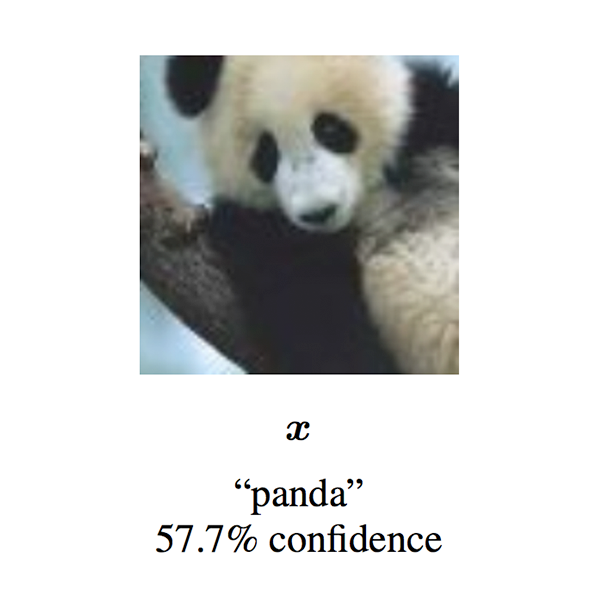
Adversarial Example Generation
Train a convolutional neural network for image classification using transfer learning.
Image/Video
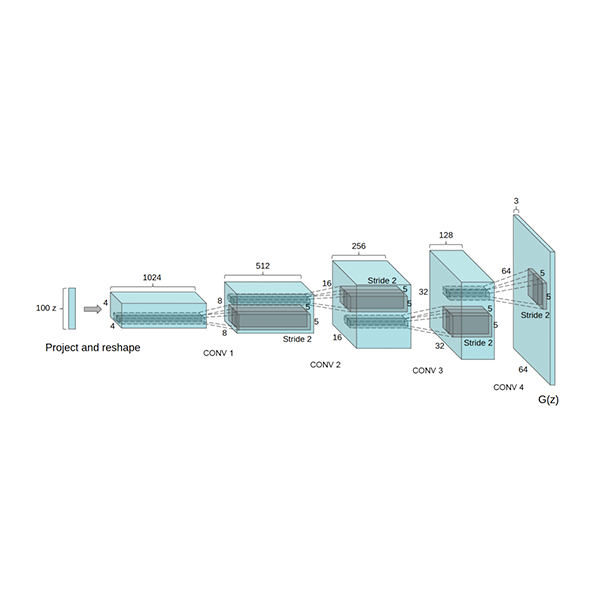
DCGAN Tutorial
Train a generative adversarial network (GAN) to generate new celebrities.
Image/Video
Spatial Transformer Networks Tutorial
Learn how to augment your network using a visual attention mechanism.
Image/Video

Audio IO
Learn to load data with torchaudio.
Audio

Audio Resampling
Learn to resample audio waveforms using torchaudio.
Audio
Audio Data Augmentation
Learn to apply data augmentations using torchaudio.
Audio
Audio Feature Extractions
Learn to extract features using torchaudio.
Audio
Audio Feature Augmentation
Learn to augment features using torchaudio.
Audio
Audio Datasets
Learn to use torchaudio datasets.
Audio
Automatic Speech Recognition with Wav2Vec2 in torchaudio
Learn how to use torchaudio’s pretrained models for building a speech recognition application.
Audio
Speech Command Classification
Learn how to correctly format an audio dataset and then train/test an audio classifier network on the dataset.
Audio

Text-to-Speech with torchaudio
Learn how to use torchaudio’s pretrained models for building a text-to-speech application.
Audio
Forced Alignment with Wav2Vec2 in torchaudio
Learn how to use torchaudio’s Wav2Vec2 pretrained models for aligning text to speech
Audio
Fast Transformer Inference with Better Transformer
Deploy a PyTorch Transformer model using Better Transformer with high performance for inference
Production,Text
![]()
Sequence-to-Sequence Modeling with nn.Transformer and torchtext
Learn how to train a sequence-to-sequence model that uses the nn.Transformer module.
Text
![]()
NLP from Scratch: Classifying Names with a Character-level RNN
Build and train a basic character-level RNN to classify word from scratch without the use of torchtext. First in a series of three tutorials.
Text
NLP from Scratch: Generating Names with a Character-level RNN
After using character-level RNN to classify names, learn how to generate names from languages. Second in a series of three tutorials.
Text
NLP from Scratch: Translation with a Sequence-to-sequence Network and Attention
This is the third and final tutorial on doing “NLP From Scratch”, where we write our own classes and functions to preprocess the data to do our NLP modeling tasks.
Text
![]()
Text Classification with Torchtext
Learn how to build the dataset and classify text using torchtext library.
Text
Language Translation with Transformer
Train a language translation model from scratch using Transformer.
Text
![]()
Reinforcement Learning (DQN)
Learn how to use PyTorch to train a Deep Q Learning (DQN) agent on the CartPole-v0 task from the OpenAI Gym.
Reinforcement-Learning

Reinforcement Learning (PPO) with TorchRL
Learn how to use PyTorch and TorchRL to train a Proximal Policy Optimization agent on the Inverted Pendulum task from Gym.
Reinforcement-Learning

Train a Mario-playing RL Agent
Use PyTorch to train a Double Q-learning agent to play Mario.
Reinforcement-Learning

Deploying PyTorch in Python via a REST API with Flask
Deploy a PyTorch model using Flask and expose a REST API for model inference using the example of a pretrained DenseNet 121 model which detects the image.
Production

Introduction to TorchScript
Introduction to TorchScript, an intermediate representation of a PyTorch model (subclass of nn.Module) that can then be run in a high-performance environment such as C++.
Production,TorchScript

Loading a TorchScript Model in C++
Learn how PyTorch provides to go from an existing Python model to a serialized representation that can be loaded and executed purely from C++, with no dependency on Python.
Production,TorchScript

(optional) Exporting a Model from PyTorch to ONNX and Running it using ONNX Runtime
Convert a model defined in PyTorch into the ONNX format and then run it with ONNX Runtime.
Production

Building a Convolution/Batch Norm fuser in FX
Build a simple FX pass that fuses batch norm into convolution to improve performance during inference.
FX
Building a Simple Performance Profiler with FX
Build a simple FX interpreter to record the runtime of op, module, and function calls and report statistics
FX
(beta) Channels Last Memory Format in PyTorch
Get an overview of Channels Last memory format and understand how it is used to order NCHW tensors in memory preserving dimensions.
Memory-Format,Best-Practice,Frontend-APIs
Using the PyTorch C++ Frontend
Walk through an end-to-end example of training a model with the C++ frontend by training a DCGAN – a kind of generative model – to generate images of MNIST digits.
Frontend-APIs,C++
Custom C++ and CUDA Extensions
Create a neural network layer with no parameters using numpy. Then use scipy to create a neural network layer that has learnable weights.
Extending-PyTorch,Frontend-APIs,C++,CUDA

Extending TorchScript with Custom C++ Operators
Implement a custom TorchScript operator in C++, how to build it into a shared library, how to use it in Python to define TorchScript models and lastly how to load it into a C++ application for inference workloads.
Extending-PyTorch,Frontend-APIs,TorchScript,C++

Extending TorchScript with Custom C++ Classes
This is a continuation of the custom operator tutorial, and introduces the API we’ve built for binding C++ classes into TorchScript and Python simultaneously.
Extending-PyTorch,Frontend-APIs,TorchScript,C++

Dynamic Parallelism in TorchScript
This tutorial introduces the syntax for doing *dynamic inter-op parallelism* in TorchScript.
Frontend-APIs,TorchScript,C++
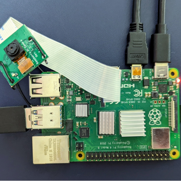
Real Time Inference on Raspberry Pi 4
This tutorial covers how to run quantized and fused models on a Raspberry Pi 4 at 30 fps.
TorchScript,Model-Optimization,Image/Video,Quantization
Autograd in C++ Frontend
The autograd package helps build flexible and dynamic nerural netorks. In this tutorial, exploreseveral examples of doing autograd in PyTorch C++ frontend
Frontend-APIs,C++

Registering a Dispatched Operator in C++
The dispatcher is an internal component of PyTorch which is responsible for figuring out what code should actually get run when you call a function like torch::add.
Extending-PyTorch,Frontend-APIs,C++
![]()
Extending Dispatcher For a New Backend in C++
Learn how to extend the dispatcher to add a new device living outside of the pytorch/pytorch repo and maintain it to keep in sync with native PyTorch devices.
Extending-PyTorch,Frontend-APIs,C++
![]()
Custom Function Tutorial: Double Backward
Learn how to write a custom autograd Function that supports double backward.
Extending-PyTorch,Frontend-APIs
![]()
Custom Function Tutorial: Fusing Convolution and Batch Norm
Learn how to create a custom autograd Function that fuses batch norm into a convolution to improve memory usage.
Extending-PyTorch,Frontend-APIs
![]()
Forward-mode Automatic Differentiation
Learn how to use forward-mode automatic differentiation.
Frontend-APIs
![]()
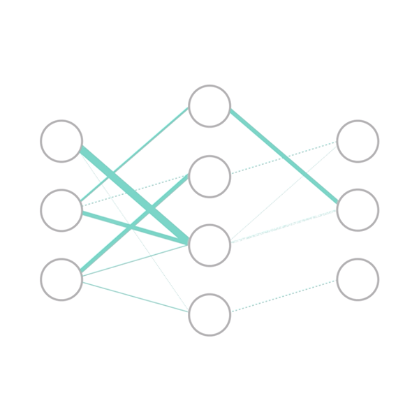
Jacobians, Hessians, hvp, vhp, and more
Learn how to compute advanced autodiff quantities using torch.func
Frontend-APIs
![]()
Model Ensembling
Learn how to ensemble models using torch.vmap
Frontend-APIs
![]()
Per-Sample-Gradients
Learn how to compute per-sample-gradients using torch.func
Frontend-APIs
![]()
Neural Tangent Kernels
Learn how to compute neural tangent kernels using torch.func
Frontend-APIs
![]()
Performance Profiling in PyTorch
Learn how to use the PyTorch Profiler to benchmark your module’s performance.
Model-Optimization,Best-Practice,Profiling

Performance Profiling in TensorBoard
Learn how to use the TensorBoard plugin to profile and analyze your model’s performance.
Model-Optimization,Best-Practice,Profiling,TensorBoard
Hyperparameter Tuning Tutorial
Learn how to use Ray Tune to find the best performing set of hyperparameters for your model.
Model-Optimization,Best-Practice

Optimizing Vision Transformer Model
Learn how to use Facebook Data-efficient Image Transformers DeiT and script and optimize it for mobile.
Model-Optimization,Best-Practice,Mobile

Parametrizations Tutorial
Learn how to use torch.nn.utils.parametrize to put constriants on your parameters (e.g. make them orthogonal, symmetric positive definite, low-rank…)
Model-Optimization,Best-Practice

Pruning Tutorial
Learn how to use torch.nn.utils.prune to sparsify your neural networks, and how to extend it to implement your own custom pruning technique.
Model-Optimization,Best-Practice
(beta) Dynamic Quantization on an LSTM Word Language Model
Apply dynamic quantization, the easiest form of quantization, to a LSTM-based next word prediction model.
Text,Quantization,Model-Optimization
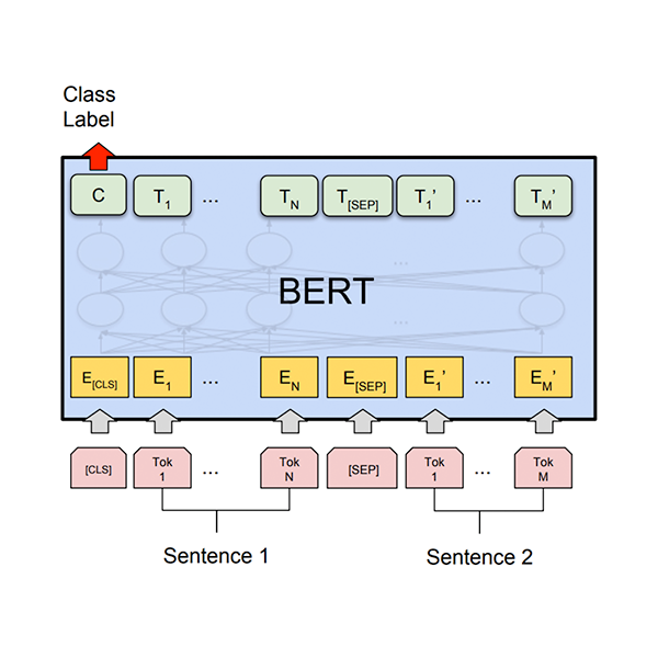
(beta) Dynamic Quantization on BERT
Apply the dynamic quantization on a BERT (Bidirectional Embedding Representations from Transformers) model.
Text,Quantization,Model-Optimization
(beta) Quantized Transfer Learning for Computer Vision Tutorial
Extends the Transfer Learning for Computer Vision Tutorial using a quantized model.
Image/Video,Quantization,Model-Optimization
(beta) Static Quantization with Eager Mode in PyTorch
This tutorial shows how to do post-training static quantization.
Quantization
Grokking PyTorch Intel CPU Performance from First Principles
A case study on the TorchServe inference framework optimized with Intel® Extension for PyTorch.
Model-Optimization,Production
![]()
Grokking PyTorch Intel CPU Performance from First Principles (Part 2)
A case study on the TorchServe inference framework optimized with Intel® Extension for PyTorch (Part 2).
Model-Optimization,Production
![]()
Multi-Objective Neural Architecture Search with Ax
Learn how to use Ax to search over architectures find optimal tradeoffs between accuracy and latency.
Model-Optimization,Best-Practice,Ax,TorchX
![]()
torch.compile Tutorial
Speed up your models with minimal code changes using torch.compile, the latest PyTorch compiler solution.
Model-Optimization
![]()
(beta) Implementing High-Performance Transformers with SCALED DOT PRODUCT ATTENTION
This tutorial explores the new torch.nn.functional.scaled_dot_product_attention and how it can be used to construct Transformer components.
Model-Optimization,Attention,Transformer
![]()
PyTorch Distributed Overview
Briefly go over all concepts and features in the distributed package. Use this document to find the distributed training technology that can best serve your application.
Parallel-and-Distributed-Training

Distributed Data Parallel in PyTorch — Video Tutorials
This series of video tutorials walks you through distributed training in PyTorch via DDP.
Parallel-and-Distributed-Training
Single-Machine Model Parallel Best Practices
Learn how to implement model parallel, a distributed training technique which splits a single model onto different GPUs, rather than replicating the entire model on each GPU
Parallel-and-Distributed-Training

Getting Started with Distributed Data Parallel
Learn the basics of when to use distributed data paralle versus data parallel and work through an example to set it up.
Parallel-and-Distributed-Training

Writing Distributed Applications with PyTorch
Set up the distributed package of PyTorch, use the different communication strategies, and go over some the internals of the package.
Parallel-and-Distributed-Training

Customize Process Group Backends Using Cpp Extensions
Extend ProcessGroup with custom collective communication implementations.
Parallel-and-Distributed-Training

Getting Started with Distributed RPC Framework
Learn how to build distributed training using the torch.distributed.rpc package.
Parallel-and-Distributed-Training

Implementing a Parameter Server Using Distributed RPC Framework
Walk through a through a simple example of implementing a parameter server using PyTorch’s Distributed RPC framework.
Parallel-and-Distributed-Training

Distributed Pipeline Parallelism Using RPC
Demonstrate how to implement distributed pipeline parallelism using RPC
Parallel-and-Distributed-Training

Implementing Batch RPC Processing Using Asynchronous Executions
Learn how to use rpc.functions.async_execution to implement batch RPC
Parallel-and-Distributed-Training

Combining Distributed DataParallel with Distributed RPC Framework
Walk through a through a simple example of how to combine distributed data parallelism with distributed model parallelism.
Parallel-and-Distributed-Training

Training Transformer models using Pipeline Parallelism
Walk through a through a simple example of how to train a transformer model using pipeline parallelism.
Parallel-and-Distributed-Training
![]()
Training Transformer models using Distributed Data Parallel and Pipeline Parallelism
Walk through a through a simple example of how to train a transformer model using Distributed Data Parallel and Pipeline Parallelism
Parallel-and-Distributed-Training
![]()
Getting Started with Fully Sharded Data Parallel(FSDP)
Learn how to train models with Fully Sharded Data Parallel package.
Parallel-and-Distributed-Training

Advanced Model Training with Fully Sharded Data Parallel (FSDP)
Explore advanced model training with Fully Sharded Data Parallel package.
Parallel-and-Distributed-Training
Image Segmentation DeepLabV3 on iOS
A comprehensive step-by-step tutorial on how to prepare and run the PyTorch DeepLabV3 image segmentation model on iOS.
Mobile

Image Segmentation DeepLabV3 on Android
A comprehensive step-by-step tutorial on how to prepare and run the PyTorch DeepLabV3 image segmentation model on Android.
Mobile

Introduction to TorchRec
TorchRec is a PyTorch domain library built to provide common sparsity & parallelism primitives needed for large-scale recommender systems.
TorchRec,Recommender

Exploring TorchRec sharding
This tutorial covers the sharding schemes of embedding tables by using EmbeddingPlanner and DistributedModelParallel API.
TorchRec,Recommender
Introduction to TorchMultimodal
TorchMultimodal is a library that provides models, primitives and examples for training multimodal tasks
TorchMultimodal
Additional Resources
Examples of PyTorch
A set of examples around PyTorch in Vision, Text, Reinforcement Learning that you can incorporate in your existing work.
Check Out Examples
PyTorch Cheat Sheet
Quick overview to essential PyTorch elements.
Open
Tutorials on GitHub
Access PyTorch Tutorials from GitHub.
Go To GitHub
Run Tutorials on Google Colab
Learn how to copy tutorial data into Google Drive so that you can run tutorials on Google Colab.
Open
beginner/basics/quickstart_tutorial

Run in Google Colab
Colab

Download Notebook
Notebook

View on GitHub
GitHub
Note
Click here
to download the full example code
Learn the Basics ||
Quickstart ||
Tensors ||
Datasets & DataLoaders ||
Transforms ||
Build Model ||
Autograd ||
Optimization ||
Save & Load Model
This section runs through the API for common tasks in machine learning. Refer to the links in each section to dive deeper.
Working with data
PyTorch has two primitives to work with data:
torch.utils.data.DataLoader and torch.utils.data.Dataset.
Dataset stores the samples and their corresponding labels, and DataLoader wraps an iterable around
the Dataset.
import torch
from torch import nn
from torch.utils.data import DataLoader
from torchvision import datasets
from torchvision.transforms import ToTensor
PyTorch offers domain-specific libraries such as TorchText,
TorchVision, and TorchAudio,
all of which include datasets. For this tutorial, we will be using a TorchVision dataset.
The torchvision.datasets module contains Dataset objects for many real-world vision data like
CIFAR, COCO (full list here). In this tutorial, we
use the FashionMNIST dataset. Every TorchVision Dataset includes two arguments: transform and
target_transform to modify the samples and labels respectively.
Downloading http://fashion-mnist.s3-website.eu-central-1.amazonaws.com/train-images-idx3-ubyte.gz
Downloading http://fashion-mnist.s3-website.eu-central-1.amazonaws.com/train-images-idx3-ubyte.gz to data/FashionMNIST/raw/train-images-idx3-ubyte.gz

  0%|          | 0/26421880 [00:00<?, ?it/s]
  0%|          | 32768/26421880 [00:00<01:25, 308059.63it/s]
  0%|          | 65536/26421880 [00:00<01:26, 303043.56it/s]
  0%|          | 131072/26421880 [00:00<00:59, 439681.08it/s]
  1%|          | 229376/26421880 [00:00<00:42, 622716.53it/s]
  2%|1         | 491520/26421880 [00:00<00:20, 1265101.23it/s]
  4%|3         | 950272/26421880 [00:00<00:11, 2266393.32it/s]
  7%|7         | 1933312/26421880 [00:00<00:05, 4470475.50it/s]
 15%|#4        | 3833856/26421880 [00:00<00:02, 8597667.83it/s]
 26%|##6       | 6946816/26421880 [00:00<00:01, 14826408.11it/s]
 37%|###7      | 9830400/26421880 [00:01<00:00, 18325880.89it/s]
 49%|####8     | 12943360/26421880 [00:01<00:00, 21430109.73it/s]
 61%|######    | 16023552/26421880 [00:01<00:00, 23472607.90it/s]
 73%|#######2  | 19169280/26421880 [00:01<00:00, 25026445.68it/s]
 84%|########4 | 22249472/26421880 [00:01<00:00, 26065062.25it/s]
 96%|#########5| 25362432/26421880 [00:01<00:00, 26792582.99it/s]
100%|##########| 26421880/26421880 [00:01<00:00, 16092036.37it/s]
Extracting data/FashionMNIST/raw/train-images-idx3-ubyte.gz to data/FashionMNIST/raw

Downloading http://fashion-mnist.s3-website.eu-central-1.amazonaws.com/train-labels-idx1-ubyte.gz
Downloading http://fashion-mnist.s3-website.eu-central-1.amazonaws.com/train-labels-idx1-ubyte.gz to data/FashionMNIST/raw/train-labels-idx1-ubyte.gz

  0%|          | 0/29515 [00:00<?, ?it/s]
100%|##########| 29515/29515 [00:00<00:00, 270168.86it/s]
100%|##########| 29515/29515 [00:00<00:00, 268807.84it/s]
Extracting data/FashionMNIST/raw/train-labels-idx1-ubyte.gz to data/FashionMNIST/raw

Downloading http://fashion-mnist.s3-website.eu-central-1.amazonaws.com/t10k-images-idx3-ubyte.gz
Downloading http://fashion-mnist.s3-website.eu-central-1.amazonaws.com/t10k-images-idx3-ubyte.gz to data/FashionMNIST/raw/t10k-images-idx3-ubyte.gz

  0%|          | 0/4422102 [00:00<?, ?it/s]
  1%|          | 32768/4422102 [00:00<00:14, 299095.68it/s]
  1%|1         | 65536/4422102 [00:00<00:14, 297990.20it/s]
  3%|2         | 131072/4422102 [00:00<00:09, 433485.30it/s]
  5%|5         | 229376/4422102 [00:00<00:06, 614892.22it/s]
 11%|#1        | 491520/4422102 [00:00<00:03, 1250662.95it/s]
 21%|##1       | 950272/4422102 [00:00<00:01, 2241530.65it/s]
 44%|####3     | 1933312/4422102 [00:00<00:00, 4417649.12it/s]
 87%|########6 | 3833856/4422102 [00:00<00:00, 8508869.61it/s]
100%|##########| 4422102/4422102 [00:00<00:00, 5003389.55it/s]
Extracting data/FashionMNIST/raw/t10k-images-idx3-ubyte.gz to data/FashionMNIST/raw

Downloading http://fashion-mnist.s3-website.eu-central-1.amazonaws.com/t10k-labels-idx1-ubyte.gz
Downloading http://fashion-mnist.s3-website.eu-central-1.amazonaws.com/t10k-labels-idx1-ubyte.gz to data/FashionMNIST/raw/t10k-labels-idx1-ubyte.gz

  0%|          | 0/5148 [00:00<?, ?it/s]
100%|##########| 5148/5148 [00:00<00:00, 27933087.96it/s]
Extracting data/FashionMNIST/raw/t10k-labels-idx1-ubyte.gz to data/FashionMNIST/raw
We pass the Dataset as an argument to DataLoader. This wraps an iterable over our dataset, and supports
automatic batching, sampling, shuffling and multiprocess data loading. Here we define a batch size of 64, i.e. each element
in the dataloader iterable will return a batch of 64 features and labels.
Shape of X [N, C, H, W]: torch.Size([64, 1, 28, 28])
Shape of y: torch.Size([64]) torch.int64
Read more about loading data in PyTorch.
Creating Models
To define a neural network in PyTorch, we create a class that inherits
from nn.Module. We define the layers of the network
in the __init__ function and specify how data will pass through the network in the forward function. To accelerate
operations in the neural network, we move it to the GPU or MPS if available.
Using cuda device
NeuralNetwork(
  (flatten): Flatten(start_dim=1, end_dim=-1)
  (linear_relu_stack): Sequential(
    (0): Linear(in_features=784, out_features=512, bias=True)
    (1): ReLU()
    (2): Linear(in_features=512, out_features=512, bias=True)
    (3): ReLU()
    (4): Linear(in_features=512, out_features=10, bias=True)
  )
)
Read more about building neural networks in PyTorch.
Optimizing the Model Parameters
To train a model, we need a loss function
and an optimizer.
In a single training loop, the model makes predictions on the training dataset (fed to it in batches), and
backpropagates the prediction error to adjust the model’s parameters.
def train(dataloader, model, loss_fn, optimizer):
    size = len(dataloader.dataset)
    model.train()
    for batch, (X, y) in enumerate(dataloader):
        X, y = X.to(device), y.to(device)

        # Compute prediction error
        pred = model(X)
        loss = loss_fn(pred, y)

        # Backpropagation
        loss.backward()
        optimizer.step()
        optimizer.zero_grad()

        if batch % 100 == 0:
            loss, current = loss.item(), (batch + 1) * len(X)
            print(f"loss: {loss:>7f}  [{current:>5d}/{size:>5d}]")
We also check the model’s performance against the test dataset to ensure it is learning.
def test(dataloader, model, loss_fn):
    size = len(dataloader.dataset)
    num_batches = len(dataloader)
    model.eval()
    test_loss, correct = 0, 0
    with torch.no_grad():
        for X, y in dataloader:
            X, y = X.to(device), y.to(device)
            pred = model(X)
            test_loss += loss_fn(pred, y).item()
            correct += (pred.argmax(1) == y).type(torch.float).sum().item()
    test_loss /= num_batches
    correct /= size
    print(f"Test Error: n Accuracy: {(100*correct):>0.1f}%, Avg loss: {test_loss:>8f} n")
The training process is conducted over several iterations (epochs). During each epoch, the model learns
parameters to make better predictions. We print the model’s accuracy and loss at each epoch; we’d like to see the
accuracy increase and the loss decrease with every epoch.
Epoch 1
-------------------------------
loss: 2.306633  [   64/60000]
loss: 2.295603  [ 6464/60000]
loss: 2.271502  [12864/60000]
loss: 2.269616  [19264/60000]
loss: 2.253280  [25664/60000]
loss: 2.218332  [32064/60000]
loss: 2.235103  [38464/60000]
loss: 2.197699  [44864/60000]
loss: 2.198300  [51264/60000]
loss: 2.167361  [57664/60000]
Test Error:
 Accuracy: 37.9%, Avg loss: 2.158536

Epoch 2
-------------------------------
loss: 2.175986  [   64/60000]
loss: 2.165268  [ 6464/60000]
loss: 2.106405  [12864/60000]
loss: 2.126396  [19264/60000]
loss: 2.074193  [25664/60000]
loss: 2.012309  [32064/60000]
loss: 2.048996  [38464/60000]
loss: 1.968931  [44864/60000]
loss: 1.975772  [51264/60000]
loss: 1.904674  [57664/60000]
Test Error:
 Accuracy: 53.4%, Avg loss: 1.901651

Epoch 3
-------------------------------
loss: 1.935737  [   64/60000]
loss: 1.909086  [ 6464/60000]
loss: 1.796208  [12864/60000]
loss: 1.841555  [19264/60000]
loss: 1.716872  [25664/60000]
loss: 1.672111  [32064/60000]
loss: 1.700074  [38464/60000]
loss: 1.599467  [44864/60000]
loss: 1.618445  [51264/60000]
loss: 1.518378  [57664/60000]
Test Error:
 Accuracy: 60.0%, Avg loss: 1.534658

Epoch 4
-------------------------------
loss: 1.597967  [   64/60000]
loss: 1.569743  [ 6464/60000]
loss: 1.423039  [12864/60000]
loss: 1.498795  [19264/60000]
loss: 1.361838  [25664/60000]
loss: 1.363473  [32064/60000]
loss: 1.379959  [38464/60000]
loss: 1.303219  [44864/60000]
loss: 1.329679  [51264/60000]
loss: 1.238595  [57664/60000]
Test Error:
 Accuracy: 62.6%, Avg loss: 1.261510

Epoch 5
-------------------------------
loss: 1.337658  [   64/60000]
loss: 1.326035  [ 6464/60000]
loss: 1.161518  [12864/60000]
loss: 1.271429  [19264/60000]
loss: 1.130588  [25664/60000]
loss: 1.159320  [32064/60000]
loss: 1.183357  [38464/60000]
loss: 1.119639  [44864/60000]
loss: 1.150976  [51264/60000]
loss: 1.074898  [57664/60000]
Test Error:
 Accuracy: 64.3%, Avg loss: 1.092475

Done!
Read more about Training your model.
Saving Models
A common way to save a model is to serialize the internal state dictionary (containing the model parameters).
Saved PyTorch Model State to model.pth
Loading Models
The process for loading a model includes re-creating the model structure and loading
the state dictionary into it.
<All keys matched successfully>
This model can now be used to make predictions.
classes = [
    "T-shirt/top",
    "Trouser",
    "Pullover",
    "Dress",
    "Coat",
    "Sandal",
    "Shirt",
    "Sneaker",
    "Bag",
    "Ankle boot",
]

model.eval()
x, y = test_data[0][0], test_data[0][1]
with torch.no_grad():
    x = x.to(device)
    pred = model(x)
    predicted, actual = classes[pred[0].argmax(0)], classes[y]
    print(f'Predicted: "{predicted}", Actual: "{actual}"')
Predicted: "Ankle boot", Actual: "Ankle boot"
Read more about Saving & Loading your model.
Total running time of the script: ( 0 minutes 51.128 seconds)
Gallery generated by Sphinx-Gallery
Если вы уже пробовали создавать собственные глубокие нейронные сети с помощью TensorFlow и Keras, то, вероятно, знакомы с чувством разочарования при отлаживании этих библиотек. Хотя они имеют API на Python, всё еще трудно выяснить, что именно пошло не так при ошибке. Они также плохо работают вместе с библиотеками numpy, scipy, scikit-learn, Cython и другими. Библиотека глубокого обучения PyTorch имеет заявленное преимущество — хорошо работает с Python и создана для апологетов Python. Кроме того, приятное свойство PyTorch — построение вычислительного динамического графа, противоположно статическим вычислительным графам, представленным в TensorFlow и Keras. PyTorch сейчас находится на подъеме и используется в разработке Facebook, Twitter, NVIDIA и другими компаниями. Давайте обратимся к туториалу по использованию PyTorch.

Перед вами перевод статьи «A PyTorch tutorial – deep learning in Python», ссылка на оригинал — в подвале статьи.
Первый вопрос для рассмотрения — действительно ли PyTorch лучше TensorFlow? Это субъективно, так как с точки зрения производительности нет больших различий. В любом случае, PyTorch стал серьезным соперником в соревновании между библиотеками глубокого обучения. Давайте начнем изучать библиотеку, оставив для размышлений вопрос о том, что же лучше.
В этом разделе мы обсудим главные идеи, стоящие за PyTorch, начиная с тензоров и вычислительных графов, заканчивая переменными классами и функциональностью автоматического дифференцирования.
Установка на Windows
Стоит сказать, если вы пользователь Windows, на веб-сайте PyTorch нет опции для простой установки библиотеки для этой операционной системы. Однако задача легко решается с помощью этого веб-сайта, где находятся дальнейшие инструкции. Установка стоит затраченных усилий.
Вычислительные графы
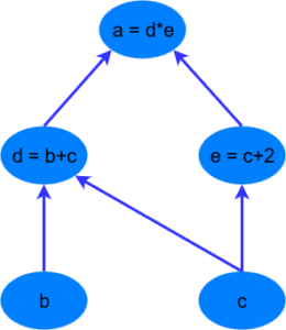
Первое, что необходимо понять о любой библиотеке глубокого обучения — идея вычислительных графов. Вычислительный граф — набор вычислений, которые называются узлами (nodes), и которые соединены в прямом порядке вычислений. Другими словами, выбранный узел зависит от узлов на входе, который в свою очередь производит вычисления для других узлов. Ниже представлен простой пример вычислительного графа для вычисления выражения a = (b + c) * (c + 2). Можно разбить вычисление на следующие шаги:
Преимущества использования вычислительного графа в том, что каждый узел является независимым функционирующим куском кода, если получит все необходимые входные данные. Это позволяет оптимизировать производительность при выполнении расчетов, используя многоканальную обработку, параллельные вычисления. Все основные фреймворки для глубокого обучения (TensorFlow, Theano, PyTorch и так далее) включают в себя конструкции вычислительных графов, с помощью которых выполняются операции внутри нейронных сетей и происходит обратное распространение градиента ошибки.
Тензоры
Тензоры — подобные матрице структуры данных, которые являются неотъемлемыми компонентами в библиотеках глубокого обучения и используются для эффективных вычислений. Графические процессоры (GPU) эффективны при вычислении операций между тензорами, что стимулировало волну возможностей в глубоком обучении. В PyTorch тензоры могут определяться несколькими способами:
import torch
x = torch.Tensor(2, 3)
Этот код создает тензор размера (2,3), заполненный нулями. В данном примере первое число — количество рядов, второе — количество столбцов:
0 0 0
0 0 0
[torch.FloatTensor of size 2x3]
Мы также можем создать тензор, заполненный случайными float-значениями:
x = torch.rand(2, 3)
Умножение тензоров, сложение друг с другом и другие алгебраические операции просты:
x = torch.ones(2,3)
y = torch.ones(2,3) * 2
x + y
Код возвращает:
3 3 3
3 3 3
[torch.FloatTensor of size 2x3]
Также доступна работа с функцией slice в numpy. Например y[:,1]:
y[:,1] = y[:,1] + 1
Которая возвращает:
2 3 2
2 3 2
[torch.FloatTensor of size 2x3]
Теперь вы знаете, как создавать тензоры и работать с ними в PyTorch. Следующим шагом туториала будет обзор более сложных конструкций в библиотеке.
Автоматическое дифференцирование в PyTorch
В библиотеках глубокого обучения есть механизмы вычисления градиента ошибки и обратного распространения ошибки через вычислительный граф. Этот механизм, называемый автоградиентом в PyTorch, легко доступен и интуитивно понятен. Переменный класс — главный компонент автоградиентной системы в PyTorch. Переменный класс обертывает тензор и позволяет автоматически вычислять градиент на тензоре при вызове функции .backward(). Объект содержит данные из тензора, градиент тензора (единожды посчитанный по отношению к некоторому другому значению, потеря) и содержит также ссылку на любую функцию, созданную переменной (если это функция созданная пользователем, ссылка будет пустой).
Создадим переменную из простого тензора:
x = Variable(torch.ones(2, 2) * 2, requires_grad=True)
В объявлении переменной используется двойной тензор размера 2х2 и дополнительно указывается, что переменной необходим градиент. При использовании этой переменной в нейронных сетях, она становится способна к обучению. Если последний параметр будет равен False, то переменная не может использоваться для обучения. В этом простом примере мы ничего не будем тренировать, но хотим запросить градиент для этой переменной, как будет показано ниже.
Далее, создадим новую переменную на основе x.
z = 2 * (x * x) + 5 * x
Чтобы вычислить градиент этой операции по x, dz/dx, можно аналитически получить 4x + 5. Если все элементы x — двойки, то градиент dz/dx — тензор размерности (2,2), заполненный числами 13. Однако сначала необходимо запустить операцию обратного распространения .backwards(), чтобы вычислить градиент относительно чего-либо. В нашем случае инициализируется единичный тензор (2,2), относительно которого считаем градиент. В таком случае вычисление — просто операция d/dx:
z.backward(torch.ones(2, 2))
print(x.grad)
Результатом является следующее:
Variable containing:
13 13
13 13
[torch.FloatTensor of size 2x2]
Заметим, это в точности то, что мы предсказывали вначале. Отметим, градиент хранится в переменной x в свойстве .grad.
Мы научились простейшим операциям с тензорами, переменными и функцией автоградиента в PyTorch. Теперь приступим к написанию простой нейронной сети в PyTorch, которая будет витриной для этих функций в дальнейшем.
Создание нейронной сети в PyTorch
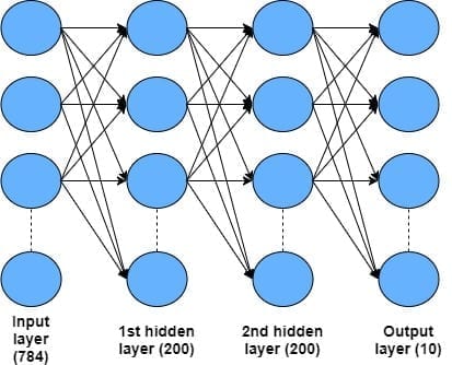
Этот раздел — основной в туториале. Полный код туториала лежит в этом репозитории на GitHub. Здесь мы создадим простую нейронную сеть с 4 слоями, включая входной и два скрытых слоя, для классификации рукописных символов в датасете MNIST. Архитектура, которую мы будем использовать, показана на картинке:
Входной слой состоит из 28 х 28 = 784 пикселей с оттенками серого, которые составляют входные данные в датасете MNIST. Входные данные далее проходят через два скрытых слоя, каждый из которых содержит 200 узлов, использующих линейную выпрямительную функцию активации (ReLU). Наконец, мы имеем выходной слой с десятью узлами, соответствующими десяти рукописным цифрам от 0 до 9. Для такой задачи классификации будем использовать выходной softmax-слой.
Класс для построения нейронной сети
Чтобы создать нейронную сеть в PyTorch, используется класс nn.Module. Чтобы им воспользоваться, необходимо наследование, что позволит использовать весь функционал базового класса nn.Module, но при этом еще имеется возможность переписать базовый класс для конструирования модели или прямого прохождения через сеть. Представленный ниже код поможет объяснить сказанное:
import torch.nn as nn
import torch.nn.functional as F

class Net(nn.Module):
   def __init__(self):
       super(Net, self).__init__()
       self.fc1 = nn.Linear(28 * 28, 200)
       self.fc2 = nn.Linear(200, 200)
       self.fc3 = nn.Linear(200, 10)
В таком определении можно видеть наследование базового класса nn.Module. В первой строке инициализации класса def __init__(self) мы имеем требуемую super() функцию языка Python, которая создает объект базового класса. В следующих трех строках создаем полностью соединенные слои как показано на диаграмме архитектуры. Полностью соединенный слой нейронной сети представлен объектом nn.Linear, в котором первый аргумент — определение количества узлов в i-том слое, а второй — количество узлов в i+1 слое. Из кода видно, первый слой принимает на входе 28×28 пикселей и соединяется с первым скрытым слоем с 200 узлами. Далее идет соединение с другим скрытым слоем с 200 узлами. И, наконец, соединение последнего скрытого слоя с выходным слоем с 10 узлами.
После определения скелета архитектуры сети, необходимо задать принципы, по которым данные будут перемещаться по ней. Это делается с помощью определяемого метода forward(), который переписывает фиктивный метод в базовом классе и требует определения для каждой сети:
def forward(self, x):
   x = F.relu(self.fc1(x))
   x = F.relu(self.fc2(x))
   x = self.fc3(x)
   return F.log_softmax(x)
Для метода forward() берем входные данные x в качестве основного аргумента. Далее, загружаем всё в в первый полностью соединенный слой self.fc1(x) и применяем активационную функцию ReLU для узлов в этом слое, используя F.relu(). Из-за иерархической природы этой нейронной сети, заменяем x на каждой стадии и отправляем на следующий слой. Делаем эту процедуру на трех соединенных слоях, за исключением последнего. На последнем слое возвращаем не ReLU, а логарифмическую softmax активационную функцию. Это, в комбинации с функцией потери отрицательного логарифмического правдоподобия, дает многоклассовую на основе кросс-энтропии функцию потерь, которую мы будет использовать для тренировки сети.
Мы определили нейронную сеть. Следующим шагом будет создание экземпляра (instance) этой архитектуры:
net = Net()
print(net)
При выводе экземпляра класса Net получаем следующее:
Net (
(fc1): Linear (784 -> 200)
(fc2): Linear (200 -> 200)
(fc3): Linear (200 -> 10)
)
Что очень удобно, так как подтверждает структуру нашей нейронной сети.
Тренировка сети
Далее необходимо задать метод оптимизации и критерий качества:
# Осуществляем оптимизацию путем стохастического градиентного спуска
optimizer = optim.SGD(net.parameters(), lr=learning_rate, momentum=0.9)
# Создаем функцию потерь
criterion = nn.NLLLoss()
В первой строке создаем оптимизатор на основе стохастического градиентного спуска, устанавливая скорость обучения (learning rate; в нашем случае определим этот показатель на уровне 0.01) и momentum. Еще в оптимизаторе необходимо определить все остальные параметры сети, но это делается легко в PyTorch благодаря методу .parameters() в базовом классе nn.Module, который наследуется из него в новый класс Net.
Далее устанавливается метрика контроля качества — функция потерь отрицательного логарифмического правдоподобия. Такой вид функции в комбинации с логарифмической softmax-функцией на выходе нейронной сети дает эквивалентную кросс-энтропийную потерю для 10 классов задачи классификации.
Настало время тренировать нейронную сеть. Во время тренировки данные будут извлекаться из объекта загрузки данных, который включен в модуль PyTorch. Здесь не будут рассмотрены детали этого способа, но вы можете найти код в этом репозитории на GitHub. Из загрузчика будут поступать партиями входные и целевые данные, которые будут подаваться в нашу нейронную сеть и функцию потерь, соответственно. Ниже представлен полный код для тренировки:
# запускаем главный тренировочный цикл
for epoch in range(epochs):
   for batch_idx, (data, target) in enumerate(train_loader):
       data, target = Variable(data), Variable(target)
# изменим размер с (batch_size, 1, 28, 28) на (batch_size, 28*28)
       data = data.view(-1, 28*28)
       optimizer.zero_grad()
       net_out = net(data)
       loss = criterion(net_out, target)
       loss.backward()
       optimizer.step()
       if batch_idx % log_interval == 0:
           print('Train Epoch: {} [{}/{} ({:.0f}%)]tLoss: {:.6f}'.format(
                   epoch, batch_idx * len(data), len(train_loader.dataset),
                          100. * batch_idx / len(train_loader), loss.data[0]))
Внешний тренировочный цикл проходит по количеству эпох, а внутренний тренировочный цикл проходит через все тренировочные данные в партиях, размер которых задается в коде как batch_size. На следующей линии конвертируем данные и целевую переменную в переменные PyTorch. Входной датасет MNIST, который находится в пакете torchvision (который вам необходимо установить при помощи pip), имеет размер (batch_size, 1, 28, 28) при извлечении из загрузчика данных. Такой четырехмерный тензор больше подходит для архитектуры сверточной нейронной сети, чем для нашей полностью соединенной сети. Тем не менее, необходимо уменьшить размерность данных с (1,28,28) до одномерного случая для 28 х 28 = 784 входных узла.
Функция .view() работает с переменными PyTorch и преобразует их форму. Если мы точно не знаем размерность данного измерения, можно использовать ‘-1’ нотацию в определении размера. Поэтому при использование data.view(-1,28*28) можно сказать, что второе измерение должно быть равно 28 x 28, а первое измерение должно быть вычислено из размера переменной оригинальных данных. На практике это означает, что данные теперь будут размера (batch_size, 784). Мы можем пропустить эту партию входных данных в нашу нейросеть, и магический PyTorch сделает за нас тяжелую работу, эффективно выполняя необходимые вычисления с тензорами.
В следующей строке запускаем optimizer.zero_grad(), который обнуляет или перезапускает градиенты в модели так, что они готовы для дальнейшего обратного распространения. В других библиотеках это реализовано неявно, но нужно помнить, что в PyTorch это делается явно. Давайте рассмотрим следующий код:
net_out = net(data)
loss = criterion(net_out, target)
Первая строка, в которой подаем порцию данных на вход нашей модели, вызывает метод forward() в классе Net. После запуска строки переменная net_out будет иметь логарифмический softmax-выход из нашей нейронной сети для заданной партии данных. Это одна из самых замечательных особенностей PyTorch, так как можно активировать любой стандартный отладчик Python, который вы обычно используете, и мгновенно узнать, что происходит в нейронной сети. Это противоположно другим библиотекам глубокого обучения, TensorFlow и Keras, в которых требуется производить сложные отладочные действия, чтобы узнать, что ваша нейронная сеть действительно создает. Надеюсь, вы поиграете с кодом для этого туториала и поймете, насколько в PyTorch удобный отладчик.
Во второй строке кода инициализируется функция потери отрицательного логарифмического правдоподобия между выходом нашей нейросети и истинными метками заданной партии данных.
Давайте посмотрим на следующие две строки:
loss.backward()
optimizer.step()
Первая строка запускает операцию обратного распространения ошибки из переменной потери в обратном направлении через нейросеть. Если сравнить это с упомянутой выше операцией .backward(), которую мы рассматривали в туториале, видно, что не используется никакой аргумент в операции .backward(). Скалярные переменные при использовании на них .backward() не требуют аргумента; только тензорам необходим согласованный аргумент для передачи в операцию .backward().
В следующей строке мы просим PyTorch выполнить градиентный спуск по шагам на основе вычисленных во время операции .backward() градиентов.
Наконец, будем выводить результаты каждый раз, когда модель достигает определенного числа итераций:
if batch_idx % log_interval == 0:
   print('Train Epoch: {} [{}/{} ({:.0f}%)]tLoss: {:.6f}'.format(
                   epoch, batch_idx * len(data), len(train_loader.dataset),
                          100. * batch_idx / len(train_loader), loss.data[0]))
Эта функция выводит наш прогресс на протяжении эпох тренировки и показывает ошибку нейросети в этот момент. Отметим, что доступ к потерям находится в свойстве .data у переменной PyTorch, которая в данном случае будет массивом с единственным значением. Получаем скалярную потерю используя loss.data[0].
Запуская этот тренировочный цикл, получаем на выходе следующее:
Train Epoch: 9 [52000/60000 (87%)] Loss: 0.015086

Train Epoch: 9 [52000/60000 (87%)] Loss: 0.015086

Train Epoch: 9 [54000/60000 (90%)] Loss: 0.030631

Train Epoch: 9 [56000/60000 (93%)] Loss: 0.052631

Train Epoch: 9 [58000/60000 (97%)] Loss: 0.052678
После 10 эпох, значение потери по величине должно получиться меньше 0.05.
Тестирование сети
Чтобы проверить нашу обученную нейронную сеть на тестовом датасете MNIST, запустим следующий код:
test_loss = 0
correct = 0
for data, target in test_loader:
   data, target = Variable(data, volatile=True), Variable(target)
   data = data.view(-1, 28 * 28)
   net_out = net(data)
# Суммируем потери со всех партий
   test_loss += criterion(net_out, target).data[0]
   pred = net_out.data.max(1)[1]  # получаем индекс максимального значения
   correct += pred.eq(target.data).sum()

test_loss /= len(test_loader.dataset)
print('nTest set: Average loss: {:.4f}, Accuracy: {}/{} ({:.0f}%)n'.format(
       test_loss, correct, len(test_loader.dataset),
       100. * correct / len(test_loader.dataset)))
Этот цикл совпадает с тренировочным циклом до строки test_loss. Здесь мы извлекаем потери сети используя свойство .data[0] как и раньше, но только все в одной строке. Далее в строке pred используется метод data.max(1), который возвращает индекс наибольшего значения в определенном измерении тензора. Теперь выход нашей нейронной сети будет иметь размер (batch_size, 10), где каждое значение из второго измерения длины 10 — логарифмическая вероятность, которую нейросеть приписывает каждому выходному классу (то есть это логарифмическая вероятность принадлежности картинки к символу от 0 до 9). Поэтому для каждого входного образца в партии net_out.data будет выглядеть следующим образом:
[-1.3106e+01, -1.6731e+01, -1.1728e+01, -1.1995e+01, -1.5886e+01, -1.7700e+01, -2.4950e+01, -5.9817e-04, -1.3334e+01, -7.4527e+00]
Значение с наибольшей логарифмической вероятностью — цифра от 0 до 9, которую нейронная сеть распознает на входной картинке. Иначе говоря, это лучшее предсказание для заданного входного объекта. В примере net_out.data таким лучшим предсказанием является значение -5.9817e-04, которое соответствует цифре “7”. Поэтому для этого примера нейросеть предскажет знак “7”. Функция .max(1) определяет это максимальное значение во втором пространстве (если мы хотим найти максимум в первом пространстве, мы должны аргумент функции изменить с 1 на 0) и возвращает сразу и максимальное найденное значение, и индекс ему соответствующий. Поэтому эта конструкция имеет размер (batch_size, 2). В данном случае, нас интересует индекс максимального найденного значения, к которому мы получаем доступ с помощью вызова .max(1)[1].
Теперь у нас есть предсказание нейронной сети для каждого примера в определенной партии входных данных, и можно сравнить его с настоящей меткой класса из тренировочного датасета. Это используется для подсчета количества правильных ответов. Чтобы сделать это в PyTorch, необходимо воспользоваться функцией .eq(), которая сравнивает значения в двух тензорах и при совпадении возвращает единицу. В противном случае, функция возвращает 0:
correct += pred.eq(target.data).sum()
Суммируя выходы функции .eq(), получаем счетчик количества раз, когда нейронная сеть выдает правильный ответ. По накопленной сумме правильных предсказаний можно определить общую точность сети на тренировочном датасете. Наконец, проходя по каждой партии входных данных, выводим среднее значение функции потери и точность модели:
test_loss /= len(test_loader.dataset)
print('nTest set: Average loss: {:.4f}, Accuracy: {}/{} ({:.0f}%)n'.format(
       test_loss, correct, len(test_loader.dataset),
       100. * correct / len(test_loader.dataset)))
После тренировки сети за 10 эпох получаем следующие результаты на тестовой выборке:
Test set: Average loss: 0.0003, Accuracy: 9783/10000 (98%)
Мы получили точность 98%. Весьма неплохо!
В туториале рассмотрены базовые принципы PyTorch, начиная c тензоров до функции автоматического дифференцирования (autograd) и заканчивая пошаговым руководством, как создать полностью соединенную нейронную сеть при помощи nn.Module.
Интересные статьи:
- Как создать чат-бота с нуля на Python: подробная инструкция
- Как создать собственную нейронную сеть с нуля на языке Python
- Как создать собственный датасет из картинок Google
import time
from tqdm.auto import tqdm
from typing import Dict, List, Tuple

def train_step(epoch: int,
               model: torch.nn.Module,
               dataloader: torch.utils.data.DataLoader,
               loss_fn: torch.nn.Module,
               optimizer: torch.optim.Optimizer,
               device: torch.device,
               disable_progress_bar: bool = False) -> Tuple[float, float]:
  """Trains a PyTorch model for a single epoch.

  Turns a target PyTorch model to training mode and then
  runs through all of the required training steps (forward
  pass, loss calculation, optimizer step).

  Args:
    model: A PyTorch model to be trained.
    dataloader: A DataLoader instance for the model to be trained on.
    loss_fn: A PyTorch loss function to minimize.
    optimizer: A PyTorch optimizer to help minimize the loss function.
    device: A target device to compute on (e.g. "cuda" or "cpu").

  Returns:
    A tuple of training loss and training accuracy metrics.
    In the form (train_loss, train_accuracy). For example:

    (0.1112, 0.8743)
  """
  # Put model in train mode
  model.train()

  # Setup train loss and train accuracy values
  train_loss, train_acc = 0, 0

  # Loop through data loader data batches
  progress_bar = tqdm(
        enumerate(dataloader),
        desc=f"Training Epoch {epoch}",
        total=len(dataloader),
        disable=disable_progress_bar
    )

  for batch, (X, y) in progress_bar:
      # Send data to target device
      X, y = X.to(device), y.to(device)

      # 1. Forward pass
      y_pred = model(X)

      # 2. Calculate  and accumulate loss
      loss = loss_fn(y_pred, y)
      train_loss += loss.item()

      # 3. Optimizer zero grad
      optimizer.zero_grad()

      # 4. Loss backward
      loss.backward()

      # 5. Optimizer step
      optimizer.step()

      # Calculate and accumulate accuracy metric across all batches
      y_pred_class = torch.argmax(torch.softmax(y_pred, dim=1), dim=1)
      train_acc += (y_pred_class == y).sum().item()/len(y_pred)

      # Update progress bar
      progress_bar.set_postfix(
            {
                "train_loss": train_loss / (batch + 1),
                "train_acc": train_acc / (batch + 1),
            }
        )


  # Adjust metrics to get average loss and accuracy per batch
  train_loss = train_loss / len(dataloader)
  train_acc = train_acc / len(dataloader)
  return train_loss, train_acc

def test_step(epoch: int,
              model: torch.nn.Module,
              dataloader: torch.utils.data.DataLoader,
              loss_fn: torch.nn.Module,
              device: torch.device,
              disable_progress_bar: bool = False) -> Tuple[float, float]:
  """Tests a PyTorch model for a single epoch.

  Turns a target PyTorch model to "eval" mode and then performs
  a forward pass on a testing dataset.

  Args:
    model: A PyTorch model to be tested.
    dataloader: A DataLoader instance for the model to be tested on.
    loss_fn: A PyTorch loss function to calculate loss on the test data.
    device: A target device to compute on (e.g. "cuda" or "cpu").

  Returns:
    A tuple of testing loss and testing accuracy metrics.
    In the form (test_loss, test_accuracy). For example:

    (0.0223, 0.8985)
  """
  # Put model in eval mode
  model.eval()

  # Setup test loss and test accuracy values
  test_loss, test_acc = 0, 0

  # Loop through data loader data batches
  progress_bar = tqdm(
      enumerate(dataloader),
      desc=f"Testing Epoch {epoch}",
      total=len(dataloader),
      disable=disable_progress_bar
  )

  # Turn on inference context manager
  with torch.no_grad(): # no_grad() required for PyTorch 2.0, I found some errors with `torch.inference_mode()`, please let me know if this is not the case
      # Loop through DataLoader batches
      for batch, (X, y) in progress_bar:
          # Send data to target device
          X, y = X.to(device), y.to(device)

          # 1. Forward pass
          test_pred_logits = model(X)

          # 2. Calculate and accumulate loss
          loss = loss_fn(test_pred_logits, y)
          test_loss += loss.item()

          # Calculate and accumulate accuracy
          test_pred_labels = test_pred_logits.argmax(dim=1)
          test_acc += ((test_pred_labels == y).sum().item()/len(test_pred_labels))

          # Update progress bar
          progress_bar.set_postfix(
              {
                  "test_loss": test_loss / (batch + 1),
                  "test_acc": test_acc / (batch + 1),
              }
          )

  # Adjust metrics to get average loss and accuracy per batch
  test_loss = test_loss / len(dataloader)
  test_acc = test_acc / len(dataloader)
  return test_loss, test_acc

def train(model: torch.nn.Module,
          train_dataloader: torch.utils.data.DataLoader,
          test_dataloader: torch.utils.data.DataLoader,
          optimizer: torch.optim.Optimizer,
          loss_fn: torch.nn.Module,
          epochs: int,
          device: torch.device,
          disable_progress_bar: bool = False) -> Dict[str, List]:
  """Trains and tests a PyTorch model.

  Passes a target PyTorch models through train_step() and test_step()
  functions for a number of epochs, training and testing the model
  in the same epoch loop.

  Calculates, prints and stores evaluation metrics throughout.

  Args:
    model: A PyTorch model to be trained and tested.
    train_dataloader: A DataLoader instance for the model to be trained on.
    test_dataloader: A DataLoader instance for the model to be tested on.
    optimizer: A PyTorch optimizer to help minimize the loss function.
    loss_fn: A PyTorch loss function to calculate loss on both datasets.
    epochs: An integer indicating how many epochs to train for.
    device: A target device to compute on (e.g. "cuda" or "cpu").

  Returns:
    A dictionary of training and testing loss as well as training and
    testing accuracy metrics. Each metric has a value in a list for
    each epoch.
    In the form: {train_loss: [...],
                  train_acc: [...],
                  test_loss: [...],
                  test_acc: [...]}
    For example if training for epochs=2:
                 {train_loss: [2.0616, 1.0537],
                  train_acc: [0.3945, 0.3945],
                  test_loss: [1.2641, 1.5706],
                  test_acc: [0.3400, 0.2973]}
  """
  # Create empty results dictionary
  results = {"train_loss": [],
      "train_acc": [],
      "test_loss": [],
      "test_acc": [],
      "train_epoch_time": [],
      "test_epoch_time": []
  }

  # Loop through training and testing steps for a number of epochs
  for epoch in tqdm(range(epochs), disable=disable_progress_bar):

      # Perform training step and time it
      train_epoch_start_time = time.time()
      train_loss, train_acc = train_step(epoch=epoch,
                                        model=model,
                                        dataloader=train_dataloader,
                                        loss_fn=loss_fn,
                                        optimizer=optimizer,
                                        device=device,
                                        disable_progress_bar=disable_progress_bar)
      train_epoch_end_time = time.time()
      train_epoch_time = train_epoch_end_time - train_epoch_start_time

      # Perform testing step and time it
      test_epoch_start_time = time.time()
      test_loss, test_acc = test_step(epoch=epoch,
                                      model=model,
                                      dataloader=test_dataloader,
                                      loss_fn=loss_fn,
                                      device=device,
                                      disable_progress_bar=disable_progress_bar)
      test_epoch_end_time = time.time()
      test_epoch_time = test_epoch_end_time - test_epoch_start_time

      # Print out what's happening
      print(
          f"Epoch: {epoch+1} | "
          f"train_loss: {train_loss:.4f} | "
          f"train_acc: {train_acc:.4f} | "
          f"test_loss: {test_loss:.4f} | "
          f"test_acc: {test_acc:.4f} | "
          f"train_epoch_time: {train_epoch_time:.4f} | "
          f"test_epoch_time: {test_epoch_time:.4f}"
      )

      # Update results dictionary
      results["train_loss"].append(train_loss)
      results["train_acc"].append(train_acc)
      results["test_loss"].append(test_loss)
      results["test_acc"].append(test_acc)
      results["train_epoch_time"].append(train_epoch_time)
      results["test_epoch_time"].append(test_epoch_time)

  # Return the filled results at the end of the epochs
  return results
import time
from tqdm.auto import tqdm
from typing import Dict, List, Tuple
def train_step(epoch: int,
model: torch.nn.Module,
dataloader: torch.utils.data.DataLoader,
loss_fn: torch.nn.Module,
optimizer: torch.optim.Optimizer,
device: torch.device,
disable_progress_bar: bool = False) -> Tuple[float, float]:
«»»Trains a PyTorch model for a single epoch.
Turns a target PyTorch model to training mode and then
runs through all of the required training steps (forward
pass, loss calculation, optimizer step).
Args:
model: A PyTorch model to be trained.
dataloader: A DataLoader instance for the model to be trained on.
loss_fn: A PyTorch loss function to minimize.
optimizer: A PyTorch optimizer to help minimize the loss function.
device: A target device to compute on (e.g. «cuda» or «cpu»).
Returns:
A tuple of training loss and training accuracy metrics.
In the form (train_loss, train_accuracy). For example:
(0.1112, 0.8743)
«»»
# Put model in train mode
model.train()
# Setup train loss and train accuracy values
train_loss, train_acc = 0, 0
# Loop through data loader data batches
progress_bar = tqdm(
enumerate(dataloader),
desc=f»Training Epoch {epoch}»,
total=len(dataloader),
disable=disable_progress_bar
)
for batch, (X, y) in progress_bar:
# Send data to target device
X, y = X.to(device), y.to(device)
# 1. Forward pass
y_pred = model(X)
# 2. Calculate and accumulate loss
loss = loss_fn(y_pred, y)
train_loss += loss.item()
# 3. Optimizer zero grad
optimizer.zero_grad()
# 4. Loss backward
loss.backward()
# 5. Optimizer step
optimizer.step()
# Calculate and accumulate accuracy metric across all batches
y_pred_class = torch.argmax(torch.softmax(y_pred, dim=1), dim=1)
train_acc += (y_pred_class == y).sum().item()/len(y_pred)
# Update progress bar
progress_bar.set_postfix(
{
«train_loss»: train_loss / (batch + 1),
«train_acc»: train_acc / (batch + 1),
}
)
# Adjust metrics to get average loss and accuracy per batch
train_loss = train_loss / len(dataloader)
train_acc = train_acc / len(dataloader)
return train_loss, train_acc
def test_step(epoch: int,
model: torch.nn.Module,
dataloader: torch.utils.data.DataLoader,
loss_fn: torch.nn.Module,
device: torch.device,
disable_progress_bar: bool = False) -> Tuple[float, float]:
«»»Tests a PyTorch model for a single epoch.
Turns a target PyTorch model to «eval» mode and then performs
a forward pass on a testing dataset.
Args:
model: A PyTorch model to be tested.
dataloader: A DataLoader instance for the model to be tested on.
loss_fn: A PyTorch loss function to calculate loss on the test data.
device: A target device to compute on (e.g. «cuda» or «cpu»).
Returns:
A tuple of testing loss and testing accuracy metrics.
In the form (test_loss, test_accuracy). For example:
(0.0223, 0.8985)
«»»
# Put model in eval mode
model.eval()
# Setup test loss and test accuracy values
test_loss, test_acc = 0, 0
# Loop through data loader data batches
progress_bar = tqdm(
enumerate(dataloader),
desc=f»Testing Epoch {epoch}»,
total=len(dataloader),
disable=disable_progress_bar
)
# Turn on inference context manager
with torch.no_grad(): # no_grad() required for PyTorch 2.0, I found some errors with `torch.inference_mode()`, please let me know if this is not the case
# Loop through DataLoader batches
for batch, (X, y) in progress_bar:
# Send data to target device
X, y = X.to(device), y.to(device)
# 1. Forward pass
test_pred_logits = model(X)
# 2. Calculate and accumulate loss
loss = loss_fn(test_pred_logits, y)
test_loss += loss.item()
# Calculate and accumulate accuracy
test_pred_labels = test_pred_logits.argmax(dim=1)
test_acc += ((test_pred_labels == y).sum().item()/len(test_pred_labels))
# Update progress bar
progress_bar.set_postfix(
{
«test_loss»: test_loss / (batch + 1),
«test_acc»: test_acc / (batch + 1),
}
)
# Adjust metrics to get average loss and accuracy per batch
test_loss = test_loss / len(dataloader)
test_acc = test_acc / len(dataloader)
return test_loss, test_acc
def train(model: torch.nn.Module,
train_dataloader: torch.utils.data.DataLoader,
test_dataloader: torch.utils.data.DataLoader,
optimizer: torch.optim.Optimizer,
loss_fn: torch.nn.Module,
epochs: int,
device: torch.device,
disable_progress_bar: bool = False) -> Dict[str, List]:
«»»Trains and tests a PyTorch model.
Passes a target PyTorch models through train_step() and test_step()
functions for a number of epochs, training and testing the model
in the same epoch loop.
Calculates, prints and stores evaluation metrics throughout.
Args:
model: A PyTorch model to be trained and tested.
train_dataloader: A DataLoader instance for the model to be trained on.
test_dataloader: A DataLoader instance for the model to be tested on.
optimizer: A PyTorch optimizer to help minimize the loss function.
loss_fn: A PyTorch loss function to calculate loss on both datasets.
epochs: An integer indicating how many epochs to train for.
device: A target device to compute on (e.g. «cuda» or «cpu»).
Returns:
A dictionary of training and testing loss as well as training and
testing accuracy metrics. Each metric has a value in a list for
each epoch.
In the form: {train_loss: […],
train_acc: […],
test_loss: […],
test_acc: […]}
For example if training for epochs=2:
{train_loss: [2.0616, 1.0537],
train_acc: [0.3945, 0.3945],
test_loss: [1.2641, 1.5706],
test_acc: [0.3400, 0.2973]}
«»»
# Create empty results dictionary
results = {«train_loss»: [],
«train_acc»: [],
«test_loss»: [],
«test_acc»: [],
«train_epoch_time»: [],
«test_epoch_time»: []
}
# Loop through training and testing steps for a number of epochs
for epoch in tqdm(range(epochs), disable=disable_progress_bar):
# Perform training step and time it
train_epoch_start_time = time.time()
train_loss, train_acc = train_step(epoch=epoch,
model=model,
dataloader=train_dataloader,
loss_fn=loss_fn,
optimizer=optimizer,
device=device,
disable_progress_bar=disable_progress_bar)
train_epoch_end_time = time.time()
train_epoch_time = train_epoch_end_time — train_epoch_start_time
# Perform testing step and time it
test_epoch_start_time = time.time()
test_loss, test_acc = test_step(epoch=epoch,
model=model,
dataloader=test_dataloader,
loss_fn=loss_fn,
device=device,
disable_progress_bar=disable_progress_bar)
test_epoch_end_time = time.time()
test_epoch_time = test_epoch_end_time — test_epoch_start_time
# Print out what’s happening
print(
f»Epoch: {epoch+1} | »
f»train_loss: {train_loss:.4f} | »
f»train_acc: {train_acc:.4f} | »
f»test_loss: {test_loss:.4f} | »
f»test_acc: {test_acc:.4f} | »
f»train_epoch_time: {train_epoch_time:.4f} | »
f»test_epoch_time: {test_epoch_time:.4f}»
)
# Update results dictionary
results[«train_loss»].append(train_loss)
results[«train_acc»].append(train_acc)
results[«test_loss»].append(test_loss)
results[«test_acc»].append(test_acc)
results[«train_epoch_time»].append(train_epoch_time)
results[«test_epoch_time»].append(test_epoch_time)
# Return the filled results at the end of the epochs
return results
PyTorch Tutorials
All the tutorials are now presented as sphinx style documentation at:
https://pytorch.org/tutorials
Contributing
We use sphinx-gallery’s notebook styled examples to create the tutorials. Syntax is very simple. In essence, you write a slightly well formatted Python file and it shows up as an HTML page. In addition, a Jupyter notebook is autogenerated and available to run in Google Colab.
Here is how you can create a new tutorial (for a detailed description, see CONTRIBUTING.md):
- Create a Python file. If you want it executed while inserted into documentation, save the file with the suffix
tutorialso that the file name isyour_tutorial.py. - Put it in one of the
beginner_source,intermediate_source,advanced_sourcedirectory based on the level of difficulty. If it is a recipe, add it torecipes_source. For tutorials demonstrating unstable prototype features, add to theprototype_source. - For Tutorials (except if it is a prototype feature), include it in the
toctreedirective and create acustomcarditemin index.rst. - For Tutorials (except if it is a prototype feature), create a thumbnail in the index.rst file using a command like
.. customcarditem:: beginner/your_tutorial.html. For Recipes, create a thumbnail in the recipes_index.rst
If you are starting off with a Jupyter notebook, you can use this script to convert the notebook to Python file. After conversion and addition to the project, please make sure that section headings and other things are in logical order.
Building locally
The tutorial build is very large and requires a GPU. If your machine does not have a GPU device, you can preview your HTML build without actually downloading the data and running the tutorial code:
- Install required dependencies by running:
pip install -r requirements.txt.
If you want to use
virtualenv, in the root of the repo, run:virtualenv venv, thensource venv/bin/activate.
- If you have a GPU-powered laptop, you can build using
make docs. This will download the data, execute the tutorials and build the documentation todocs/directory. This might take about 60-120 min for systems with GPUs. If you do not have a GPU installed on your system, then see next step. - You can skip the computationally intensive graph generation by running
make html-noplotto build basic html documentation to_build/html. This way, you can quickly preview your tutorial.
If you get ModuleNotFoundError: No module named ‘pytorch_sphinx_theme’ make: *** [html-noplot] Error 2 from /tutorials/src/pytorch-sphinx-theme or /venv/src/pytorch-sphinx-theme (while using virtualenv), run
python setup.py install.
Building a single tutorial
You can build a single tutorial by using the GALLERY_PATTERN environment variable. For example to run only neural_style_transfer_tutorial.py, run:
GALLERY_PATTERN="neural_style_transfer_tutorial.py" make html
or
GALLERY_PATTERN="neural_style_transfer_tutorial.py" sphinx-build . _build
The GALLERY_PATTERN variable respects regular expressions.
About contributing to PyTorch Documentation and Tutorials
- You can find information about contributing to PyTorch documentation in the
PyTorch Repo README.md file. - Additional information can be found in PyTorch CONTRIBUTING.md.