вперед от:https://blog.csdn.net/lidahuilidahui/article/details/99679554
01-Snap и Snappy Invelocment and Installation
- Предисловие
- О Snap
-
- SNAP ВВЕДЕНИЕ
-
- STEP
- SNAP
- Sentinel Toolbox:
- Подвести итог
- SNAP Установка
- Связанные ресурсы:
- О Snappy
-
- Сносы
- Snappy Installation
-
- Поколение Snappy Package
-
- Метод 1 —- непосредственно сгенерирован путем установки SNAP:
- Метод 2 —- Используйте скрипт Snappy-Conf.bat для создания
- Шнульная интерпретация упаковки
- Snappy Package Test
- Вывод
- использованная литература
(Оригинальная статья, пожалуйста, укажите источник, спасибо!)
Предисловие
Эта статья является первым сообщением в блоге «Snap and Snappy» столбца. Благодаря сильной поддержке Европейского космического агентства (ESA), мы можем использовать большое количество получения более качественных данных о бесплатном зондировании (например: Sentinel-1, Sentinel-3 и т. Д.), И европейское бюро воздуха самостоятельно имеет самостоятельно независимо Разработал платформу обработки данных с открытым исходным кодом, которая совместима с этими данными удаленного зондирования. Программное обеспечение Snap с открытым исходным кодом объясняет дух «Open World, Free Science», который приносит удобство для исследователей, связанных с дистанционным зондированием, так что анализ обработки данных дистанционного зондирования может быть лучше разработан. существуетSnap Office ForumСоответствующие эксперты, которые вступили в контакт с Европейским воздушным бюро почувствовали свои твердые и глубокие знания и дух свободной и открытости. В то же время они чувствовали, что на форуме соответствующие научные исследователи в моей стране не обратили достаточно внимания. Большая часть программного обеспечения для обработки в области дистанционного зондирования была монополизирована ENVI, ERDAS, PCI и ARCGIS ForEEENTEMENT SENSING Company. Sensing Software Shape, QGIS и т. Д., Который не способствует избавлению от зависимости от заругания. Цель создания колонки «Snap and Snappy» в основном состоит в том, чтобы содействовать использованию и разработке программного обеспечения для обработки дистанционного зондирования с открытым исходным кодом, а также изучения его расширенной технологии обработки и основных алгоритмов, чтобы лучше обслуживать внутреннюю индустрию дистанционного зондирования в будущее. Последующее содержание столбца будет введено в программное обеспечение с открытым исходным кодом, такое как программное обеспечение с открытым исходным кодом и QGIS, и использовать меньше или даже любое коммерческое программное обеспечение.
О Snap
Дисциплины, связанные с дистанционным зондированием, которые использовали серию данных Sentinel, должны быть подвергнуты этому программному обеспечению SNAP. В Интернете также есть некоторые статьи, но независимо от глубины или широты, преимущество SNAP не может быть отражено далеко. Немногие. несмотря на то чтоОфициальный сайт Bureau Bureau Oukong SnapЕсть много информации о учебниках SNAP, но это вызвало определенные трудности из -за отсутствия соответствующих базовых знаний.
SNAP ВВЕДЕНИЕ
STEP
При поддержке проекта SEOM (научная эксплуатация операционных миссий) он разрабатывает бесплатный и с открытым исходным кодом для глобального спутника научных наблюдений (в основном спутник серии Sentinel). Бюро Eukong помещает эти наборы инструментов, которые открывают исходный код вSTEP(Scientific Toolbox Exploitation Platform)Эта платформа сообщества ESA используется для интервью научных исследователей, загрузки и использования программного обеспечения, связанного с платформой и их документов, общения с разработчиками, диалога в научном сообществе, содействие обмену и улучшению результатов и материалов.
SNAP
Большая часть следующего контента происходит отЗнайте колонку Стражного изображения «Программное обеспечение плана Copernicus -SNAP»Эта статья более полно введена (на самом деле, если вы просмотрели официальный веб -сайт SNAP, содержание статьи в основном переведено на официальный веб -сайт), и изменяется и дополняет некоторые из контента. Большая часть следующего контента происходит отЗнайте колонку Стражного изображения «Программное обеспечение плана Copernicus -SNAP»Эта статья более полно введена (на самом деле, если вы просмотрели официальный веб -сайт SNAP, содержание статьи в основном переведено на официальный веб -сайт), и изменяется и дополняет некоторые из контента.
Инструментарий ESA поддерживает обработку спутниковых данных миссии ERS-Evisat, задачи Sentinel 1/2/3 и серию национальных и сторонних задач. Эти три набора инструментов называются Sentinel 1, 2 и 3 набора инструментов, и они делятся публичной архитектурой под названием SNAP.
Предшественник Snap происходит от функций некоторых исторических наборов инструментов, разработанных в последние несколько лет, например, какBEAM、NEST(Next Esa Sar Toolbox)а такжеOrfeo Toolbox。Если вы обратите внимание на некоторые из ранних статей удаленного зондирования, вы сможете увидеть это программное обеспечение (набор инструментов).
SNAP(Sentinel Application Platform)Это платформа приложений для данных Sentry. Это базовая платформа (публичная архитектура) всех наборов инструментов, которая является платформой C-S со стороны рабочего стола. Он имеет масштабируемость, переносимость и модульный интерфейс.
Главная особенность:
- Общая архитектура всех наборов инструментов;
- Может достичь быстрого отображения и навигации гигабитных изображений;
- Графическая структура обработки (GPF): используется для создания пользовательской цепочки обработки;
- Управление расширенным уровнем: разрешить новые слои суперпозиции добавлять и работать, например, другие изображения полосы, изображения с WMS Server или Shapefile ESRI;
- Богатые заинтересованные области определения ROI, статистика и различные торговые точки;
- Простой расчет группы и суперпозиция;
- Используйте гибкое математическое выражение;
- Точная повторная деятельность и положительная стрельба общей проекции карты;
- Используйте наземные контрольные точки для географического кодирования и отделки;
- Автоматическая SRTM DEM скачать и выберите;
- Библиотека продуктов для сканирования с высокой эффективностью и крупных архивов;
- Многочисленная и многочисленная поддержка процессоров;
- Интегрированная визуализация по всему миру;
Технология, используемая в Snap:
NetBeans platform- настольная платформа приложения;
Install4J- много -платформная установка;
GeoTools- Географическая библиотека инструментов для анализа космического пространства;
GDAL- Чтение и написание сетки, векторные данные;
Jira- отслеживание вопросов;
Git- Управление версией, в хостинге в записи GitHub
Sentinel Toolbox:
- Sentinel-1 Toolbox (S1TBX)
- Большинство характеристик инструментального ящика Nest унаследовали и расширили набор инструментов Nest, которые в основном используются для обработки данных SAR: стандарт излучения, связанные с ними лечение, коррекцию местности, коррекция эллипсоидов, переизопасность, анализ синхронизации, разложение поляризации, классификация, интерференция , интерференционные ожидания обработки
- Поддерживаемые спутниковые данные SAR: Sentinel-1, ERS-1 и 2, Envisat, Alos Palsar, Terrasar-X, Cosmo-Skymed, Radarsat-2 и другие сторонние данные SAR;
- Sentinel-2 Toolbox (S2TBX)
- В основном он используется для обработки многоспектрических данных, включая маску, резку, тяжелую выборку, статистику гистограммы, анализ спектра, тяжелую проекцию, операции полосы, многочисленные операторы индекса (такие как NDVI, NDWI, LAI, CCC и т. Д.) надзор и надзор и надзор, и есть много операций, таких как классификация надзора
- Поддержка многоспектральных спутниковых данных: Sentinel-2, Envisat (Meris and Aatsr), ERS (ATSR), Rapideye, Spot, Modis (Aqua and Terra), Landsat (TM), Avnir & Prism of Alos;
- Sentinel-3 Toolbox (S3TBX)
- Поддержка визуализации данных (пирамида сетки, настройки сетки, лента слоя и т. Д.), Анализ данных (представление раздела, рассеянная карта точек, связанный анализ), обработка данных сетки (тяжелая проекция, инкрустация, кластер, классификация) обработка и т. Д.
- Поддержка типов данных: OLCI и SLSTR, Envisat (Meris and Aatsr), ERS (ATSR), SMOS, MODIS (Aqua и Terra), Landsat (TM), Landst (Avnir &), Prism и т. Д.
- SMOS Toolbox
- Поддержка данных из спутников влажности почвы и солености океана (SMOS), которые поддерживают пользователей (SMO)
- Proba-V Toolbox
- Поддержать пользователей для обработки данных, полученных спутником Proba-V (разработка спутника Proba-V является последующей работой 15-летней задачи наблюдения за точечной эветацией, а также для подготовки к недавно выпущенному Sentinel- 3 Миссия Стеллита Земли и Морского наблюдения. Работа.)
- PolSARPro: Программное обеспечение PolsarPro предложило большое количество известных алгоритмов и инструментов Pol-SAR, которые заложили основу для научного развития и использования технологии измерения поляризации, и использовали Pol-SAR, Pol-NSAR, Pol-Tomosar, Pol-TimeMesar Data Stemulus Research и разработка приложений, он должен быть более знаком с направлением направления исследования Полсара.
- Третий -сторонник -плагин -ин
- Sen2cor: Sentinel-2 L2A генерация продукта и процессор форматирования;Он имеет коррекцию атмосферы, местности и броска входных данных атмосферы L1CСущность SEN2COR создает нижнюю атмосферу, дополнительную местность и обмотки, чтобы отразить изображения; кроме того, она также создаст изображение воздушной оптической толщины, водяного пара, карт классификации сцен и вероятность облака с качественными показателями. Формат продукта его вывода такой же, как и формат пользовательского продукта L1C: изображение формата JPEG 2000, три разных разрешения, 60, 20 и 10 м. Сущность
- Sen2Three: Процессор уровня Sentienl-2 L3, который используется для синтеза изображения временной последовательности для атмосферного коррекционного изображения Sentinel-2 L2A. Все «плохие» пиксели постепенно заменяются «хорошими» пикселями последующей сцены и Синтетическое выходное изображение генерируется.Он может получить данные Sentinel-2 L2A для облачной обработки。
- Sen2Res: Процессор, который увеличивает пространственное разрешение продукта Sentinel-2 до 10 м/пикселей, что может поддерживать отражательную способность продукта.Sentinel-2 MSI не имеет полноцветной группы, Но он содержит 4 10 м/пиксельные полосы. Принцип работы SEN2RES состоит в том, чтобы создать модель, которая описывает, как делиться информацией между этими полосами (то есть контентом пикселя, независимо от отражательной способности), и какая информация специфична для этих полос (то есть цвет контента пикселя). Затем используйте эту модель, чтобы демодировать полосу 20 м/пикселей и полосу 60 м/пиксель, сохраняя при этом ее отражение.
- SNAPHU: Stanford University разработал инструменты для свободной фазы для Insar, которые могут быть интегрированы в SNAP для фазового решения для продуктов Sentinel-IW SLC.
Подвести итог
Фактически, Snap — это универсальная архитектура всех наборов инструментов Sentinel и инструментов SMOS. Архитектура SNAP является идеальной архитектурой для обработки данных и анализа миссии Earth Obervice. У нее есть следующие технологические инновационные точки:Расширение, переносимость, богатая модульная клиентская платформа, Гео (Земля Оберсерская) Абстрактная модель данных, многоуровневая структура управления памятью и графическую структуру (GPT)
Выдающееся преимущество Snap:
- Открытый исходный код (лицензия GPLV3), используйте Java Universal Framework Development
- Спутниковая платформа обработки Sentinel серии оригинальной экологии
- Поддержка графической структуры обработки (GPT).
- Плагин масштабируемого исходного кода Java/Python (Snappy)
- Поддержка двигателя и облачной платформы
- Соло -платформная установка
Для исследователей дистанционного зондирования нашей страны основным недостатком является:
- Не поддерживайте обработку внутренних спутниковых данных на данный момент;
- Многие материалы английский;
- Некоторые операции могут быть не идеальными, а операция более хлопотна.
Короче говоря, SNAP — это отличное программное обеспечение для обработки дистанционного зондирования с открытым исходным кодом, которое стоит изучать и исследовать.
SNAP Установка
Snap был обновлен до версии 7.0Я все еще использую старую версию Snap, рекомендуется обновлять. Фактически, Snap V8.0 вступил в стадию разработки.
SNAP USER DAY Conference (SNAP User Day) Будет проходить 10 сентября 2019 года: В то время эксперт по разработке Snap European Air Bureau примет участие в конференции и ответит на соответствующие вопросы Snap. Я поделюсь хардкорными сухими товарами. Если вам интересно, вы должны обратить внимание.
Загрузите URL -адрес snap v7.0:http://step.esa.int/main/download/snap-download/Сущность Рекомендуется выбрать пакет установки в форме All Toolboxes и сохранить проблемы с установкой некоторых плагин в будущем.
Установка Snap относительно проста.
Блогер в настоящее время использует систему Windows. Ключ шага под системой Windows ниже.
Щелкните левой кнопкой мыши, чтобы загрузить ESA-SNAP_ALL_WINDOWS-X64_7_0.exe (это файл .exe в системе Windows).
Вы можете выбрать путь установки:
Вы можете выбрать установку инструментов, просто по умолчанию.

Выберите, следует ли установить ярлыки и каталог меню, просто по умолчанию.
Если вы установили версию Python (v2.7, v3.3-3.4) перед установкой Snap, Python 3.4.4 используется блоггерами, если вы не устанавливаете Python, вы можете удалить крючки в маленькой квадратной раме. для Snappy File на данный момент. Также можно установить Snap, прежде чем Snappy. Под предпосылкой установки Python вы можете напрямую настроить Snappy: После установки вы можете найти следующие файлы в C: users xxxx.snap snappython path (xxxxxx представляет имя пользователя):
Обычно установлено последующее наблюдение, и на рабочем столе будет генерироваться ярлыки с защелкиванием.
После открытия SNAP, как показано на рисунке:
Связанные ресурсы:
Snap Source Code:https://github.com/senbox-org
Официальный форум SNAP:https://forum.step.esa.int/
Официальный вики -блог Snap:https://senbox.atlassian.net/wiki/spaces/SNAP/overview
Отслеживание версии Snap:https://senbox.atlassian.net/secure/Dashboard.jspa
Snap Engine Java API документ:
http://step.esa.int/docs/v6.0/apidoc/engine/
Snap Desktop Java API документ:http://step.esa.int/docs/v6.0/apidoc/desktop/
О Snappy
Сносы
Как упоминалось ранее, Snap написан в исходном коде Java, и он должен быть разработан с помощью Java для написания программ. Однако, учитывая огромное количество пакетов функций и библиотек в текущем мире с открытым исходным кодом, Snap предоставляет модуль интерфейса Python API для полного использования большого количества высококачественных модулей Python.
, Snap ( (( (( ( sentinel-1, sentinel-2 ) 、 、 , python ( ( ( 、 Scipy, Matplotlib, GDAL, Scikit-Learn) быстро реализует различные пользовательские операции и передовые алгоритмы, такие как сегментация, объектно-ориентированная классификация, классификация CNN и т. Д.。
Существует также два типа резких пакетов, один — CPYTHON (стандартный Python), а другой — Jython. Два типа имеют свои преимущества и недостатки. См. Официальное введение SNAP:https://senbox.atlassian.net/wiki/spaces/SNAP/pages/19300362/How+to+use+the+SNAP+API+from+Python
CPython:
- Если вам нужно использовать библиотеку научных расширения Python, такую как Numpy, Scipy, Matplotlib и т. Д.
- У вас уже есть код CPYTHON, вы хотите объединить функции в SNAP;
- Вы планируете реализовать быструю заглушку процессора данных -в Python;
- Вы не собираетесь разработать расширение пользовательского интерфейса настольного интерфейса Snap;
- Вам не нужно иметь полную портативность на всех платформах;
- Ваш код зависит от (или он будет зависеть от) многих нестандартных библиотек.
Если у вас есть вышеупомянутые потребности, установите Snappy of Standard Python (CPYTHON).
Jython:
- Вы планируете разрабатывать расширение пользовательского интерфейса настольного интерфейса Snap;
- Вы должны быть полностью портативными на всех платформах;
- Не нужно предоставлять мощную мощность обработки данных массива/сетки, обеспечиваемой Numpy (потому что Jython не может поддержать их);
Ввиду приведенных выше характеристик, нет сомнений в том, чтобы выбрать резкую установку CPYTHON, потому что мы хотим использовать большое количество сторонних пакетов (Numpy, Scipy, Scikit-Learn и т. Д.).)
В настоящее время большинство людей на форуме Snap установлены с Snappy Cpython Type. Следующее введено для установки Snappy type Cpython (блоггеры используют систему Win10).
Snappy Installation
Есть две основные установки Snappy:
- Поколение Snappy Package
- Шнульная интерпретация упаковки
Поколение Snappy Package
Метод 1 —- непосредственно сгенерирован путем установки SNAP:
См. Учебное пособие по установке SNAP впереди и настройте его непосредственно в процессе установки SNAP, при условии, что вы установили Python (v2.7, v3.3-3.4).
Видя это, вы можете спросить, можете ли вы установить более высокую версию Python (Python3.4 выше) и теперь ответить на ваш вопрос, три версии Python (v2.7, v3.3-3.4) являются европейски Бюро официально протестировано Европейским воздушным бюро. Лучше всего использовать эти три версии. Кроме того, форум также использует Python3.5 и 3.6 для успешной установки, но он не может гарантировать, есть ли в нем некоторые коды. Высокая версия Python3.7-3.8, никто еще не установил ее, вы можете попробовать самостоятельно. Нет сомнений в том, что высокая версия Python будет улучшена позже, но это займет только определенное время
Конфигурация владельца блога (или предложение):
Не рекомендуется использовать версию Python 2, эта версия остановит техническое обслуживание в 2020 году в Python.Две версии Python, используемые блоггерами, являются стандартной версией Python 3.4.4 (версия Python 3.4 также потеряла поддержку, но Python3.4) и Anaconda’s Python3.6.77.7Сущность Используя Python 3.6, чтобы не отставать от официальной быстрой итерации и обновления Python, потому что некоторые библиотеки (такие как GDAL и другие библиотеки) ниже Python 3.4 потеряли поддержку. С другой стороны, использование Python 3.4 для предотвращения некоторых операций от Python 3.6. Если не произойдет случайность, блоггер будет использовать Python 3.6 для представления.
- Давайте поговорим о проблеме Python 3.4.4: Официальный веб -сайт Python предоставляет только исходный код Python 3.4.5 -10, и вам необходимо скомпилировать (исходный код Python записан в C) для установки, и если вы компилируете в Windows Система, вам необходимо установить против 2010 (Visual Studio 2010), более высокая версия VS, по -видимому, составлена. Хотя компиляция не является проблемной, пакет VS -установка слишком велика (она занимает много места для хранения после установки). Таким образом, блоггер должен был использовать хорошо сочетающуюся версию Python 3.4.4, предоставленная официальным веб -сайтом Python, чтобы сэкономить проблемы. См. Веб -сайт:
https://www.python.org/downloads/release/python-344/
Нажав на этот URL, вы можете увидеть скомпилированный файл установщика MSI. Просто установите его сразу после загрузки.
- Кроме того, установка Python 3.6: Блоггер использует последнюю версию Anaconda, которая предварительно установилась с Python 3.7. Необходимо порекомендовать виртуальную среду Python 3.6. Слишком много таких учебных пособий. Я не буду повторять ее . Просто вставьте учебник случайно:https://blog.csdn.net/Fhujinwu/article/details/85851587
- Spder Anaconda, Justyter Notebook и другие редакторы иногда не удобны для автоматического заполнения. Вы также можете использовать Pycharm в качестве редактора IDE. Pycharm настраивает множество учебных пособий в Интернете, и вы можете просто вставить один:https://blog.csdn.net/wingygrandam/article/details/79378286

Метод 2 —- Используйте скрипт Snappy-Conf.bat для создания
Вы можете увидеть файл скрипта Snapp-conf.bat в пути установки SNAP (то есть путь, который вы настраиваете установку).
(Существует также инструмент командной строки GPT, который может помочь Snappy лучше обрабатывать код и представить его позже.)
Обратите внимание, что вам нужно вызвать командную строку (CMD), где находится каталог сценария Snappy-Conf.Bat, чтобы непосредственно использовать следующую команду.。
Команда конфигурации заключается в следующем:
snappy-conf <python-exe> <snappy-dir>
- 1
<p y t h o nАбсолютный путь интерпретатора Python (файл python.exe)Обратите внимание, что это должен быть абсолютный путь.
<s n a p p y i d i r> <sappood-dir> <sappay-dir> Путь каталога сгенерированного пакета. Вообще говоря /под содержимым. Это дополнительный параметр. Если вакансия является вакантной, она будет сгенерирована в C: users xxxxx.snap Snap-Python Directory (xxxxxx-это имя пользователя).
Python 3.4 В качестве примера:
Абсолютный путь шнурского файла блоггера-conf.bat (см. Выше):
E:SNAPinstall_pathsnapbinsnappy-conf.bat
Абсолютный путь, где Python 3.4 блоггера, файл python.exe ::
C:Python34python.exe

Абсолютный путь к размещению пакета:
C:Python34Libsite-packages
Итак, команда Snappy Package Generation Generation:
E:SNAPinstall_pathsnapbinsnappy-conf.bat C:Python34python.exe C:Python34Libsite-packages
- 1
Команда очень длинная, вы можете создать новый файл .txt, написать команду и скопировать его в командную строку. Блоггер был настроен очень рано и не сохранил скриншот. Вставьте официальный скриншот. Обратите внимание, что путь должен быть изменен на ваш собственный:
Поговорите об Python3.6 Анаконды :6:
Если вы используете виртуальную среду Anaconda для установки Python3.6, вы найдете папку ENVS в каталоге установки Anaconda. Вы можете установить виртуальную среду, такую как название виртуальной среды арендодателя как PY36, так что вы можете Найдите следующий каталог:
После входа в этот каталог вы можете найти Python.exe (интерпретатор):
Нестандартная библиотека виртуальной среды Python3.6 также находится под относительным путем Lib Site-Packages:
Блогер настраивает Snappy использует Windows PowerShell (Win10 Command Line Shell Shell (Win10 Command Line Shell, команда немного похожа на команду Linux System CSH (C Shell) в каталоге, где находится Snappy-Conf.Bat, но он не поддерживается , немного ребра, но он также может выполнить сценарий скрипта скрипта скрипта .bat сценария скрипта скрипта скрипта скрипта скрипта скрипта сценария скрипта), если вы запускаете PowerShell в текущем каталоге Win10, например, блоггер В каталоге Snappy-Conf.Bat:
Переместите строку меню файла в левом верхнем левом углу мыши, вы можете увидеть: Если вы нажмете на левую кнопку мыши, вы можете открыть ее. Это очень удобно. Похоже, это:
Текущий путь будет вызван ранее
Команда Snappy заключается в следующем:
Запустите файл сценария .bat или. После успеха, как показано на рисунке ниже
В то же время вы можете перейти на путь конфигурации и увидеть папку ниже:
Шнульная интерпретация упаковки
Один шаг — это один шаг, соответствующий интерпретатор Python необходим для интерпретацииsetup.py из резкого пакетаЧтобы позволить интерпретатору Python идентифицировать его как соответствующую библиотеку модулей (это задание обычно может быть завершено с помощью команды PIP, но оно не может быть здесь).Обратите внимание, что это должен быть соответствующий интерпретатор, в противном случае может быть установлена неправильная позиция. Не может установить с командой PIP。
Команда интерпретации:
<python-exe> setup.py install
- 1
<p y t h o n e x e> <python-exe> <python-exe> является соответствующим интерпретатором Python, лучше всего использовать абсолютный путь.
Setup.py расположен в резком каталоге, сгенерированном предыдущим шагом
Путь, в котором текущий путь настроен на предыдущем шаге, вы увидите файл setup.py (меньше файлов, которые вы можете увидеть, потому что это папка после успеха интерпретации), вы увидите сумки JPY (мост Java-Python Bridge , Java-Python Bridge), этот очень важный пакет. В будущем вы увидите, что многие операции будут использовать его.
Например, блоггеры используют виртуальную среду Anaconda Python3.6, соответствующий интерпретатор python.exe, где полный путь: e: anaconda anaconda3 envs py36 python.exe.
Следовательно, команда интерпретации:
E:AnacondaAnaconda3envspy36python.exe setup.py install
- 1
После успешной интерпретации, как показано на рисунке ниже
Snappy Package Test
Чтобы проверить, успешно ли установлен Snappy, вы можете проверить его с помощью простого небольшого кода.
Существует папка TestData под сгенерированной резкой, вы увидите файл тестовых данных в формате .dim.

Блоггер написал простую тестовую программу, написанную в среде Python 3.6 (обратите внимание, что file_path-это полный абсолютный путь каталога, где находятся тестовые данные. Конечно, вы также можете использовать данные Sentinel-1 Sentinel-2 для тестирования. ):
from snappy import ProductIO
file_path = r'E:AnacondaAnaconda3envspy36LibsitepackagessnappytestdataMER_FRS_L1B_SUBSET.dim'
p = ProductIO.readProduct(file_path)
list(p.getBandNames())
# print(list(p.getBandNames()))
- 1
- 2
- 3
- 4
- 5
Результаты после успеха показаны на рисунке ниже:

Если вы выполняете вышеуказанные процедуры, ошибки нет, поздравляю с вашей успешной установкой Snappy.
Пожалуйста, посмотрите об учебном пособии Snappy:
https://github.com/techforspace/sentinel
Вывод
Введение и установка Snap and Snappy должны быть закончены. Однако путь разведки и разработки Snap только что имел отправную точку, и долгий путь будет сопровождать вас! Все еще упоминайте об этом, если вы заинтересованы в Snap или Snappy, вы можете присоединиться к созданному блоггеруБюро Эйконг Бюро обмена обработки обмена: 665903216 (эта группа заполнена), европейская группа по обработке обработки воздуха (2): 1102493346。
использованная литература
[1] Шаг официальный веб -сайт:http://step.esa.int/main/
[2] Знание столбца изображения Sentinel «Поддержка программного обеспечения плана Copernicus -SNAP»:https://zhuanlan.zhihu.com/p/61230869
[3] Блог Wiki Snap:https://senbox.atlassian.net/wiki/spaces/SNAP/pages/24051781/Using+SNAP+in+your+programs
[4] Официальный веб -сайт TechForsApce:https://www.techforspace.com/
Перевод оригинального учебника SAR Basics with the Sentinel-1 Toolbox Copyright © 2015 Array Systems Computing Inc. http://www.array.ca/ https://sentinel.esa.int/web/sentinel/toolboxes
При переводе скриншоты и названия элементов управления программного обеспечения приведены в соответствие с ESA SNAP Desktop версии 2.0 с установленным набором инструментов Sentinel-1 Toolbox (S1TBX) версии 2.0. Перевод выполнен максимально приближенно к оригиналу, из-за чего некоторые формулировки могут выглядеть «коряво».
Целью этого учебника является обеспечение начинающих и опытных пользователей дистанционного зондирования пошаговыми инструкциями по работе с данными РСА в Sentinel-1 Toolbox.
Для получения более подробной информации о параметрах оператора и алгоритмических описаний, пожалуйста, обратитесь к онлайн-помощи, доступной непосредственно в программном обеспечении.
С помощью этого учебника вы научитесь калибровать, выполнять процедуру некогерентного накопления (англ. multilook), фильтровать спекл-шум и делать поправку на местность для данных, полученных с РСА.
Содержание
- 1 Пример данных
- 2 Открытие продукта
- 3 Калибровка данных
- 4 Некогерентное накопление (multilooking)
- 5 Фильтрация спекл-шума
- 6 Корректировка по местности
[править] Пример данных
Примеры данных для продукта RADARSAT-2 Fine Quad-Pol, поставляемых MDA, можно найти по адресу:
- ftp://rsat2:yvr578MM@ftp.mda.ca/Vancouver Dataset
В этом учебнике мы будем использовать набор данных «Vancouver Fine Quad2 SLC». Город Ванкувер в Британской Колумбии является третьим по величине мегаполисом в Канаде, расположенным на побережье Тихого океана.
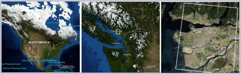
Расположение области покрытия на карте мира
Скачайте и распакуйте продукт Vancouver_R2_FineQuad2_HH_VV_HV_VH_SLC.
Все права на продукты и данные RADARSAT-2 принадлежат MacDonald, Dettwiler and Associates.
[править] Открытие продукта
Шаг 1 — открытие продукта: Используйте кнопку ![]() Open Product на панели инструментов и откройте папку с продуктом Vancouver Fine Quad RADARSAT-2.
Open Product на панели инструментов и откройте папку с продуктом Vancouver Fine Quad RADARSAT-2.
Выберите файл product.xml и нажмите Open Product.
Если вы не распаковывали архив, то можно открыть продукт, просто выбрав файл архива.
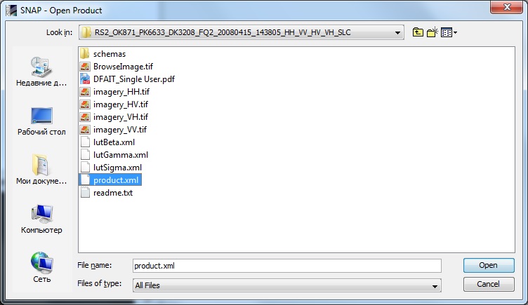
Открываем файл product.xml
Во вкладке Product Explorer вы увидите открытые продукты. Каждый продукт состоит из метаданных и растровых каналов, а также может содержать дополнительную информацию, такую как сеть точек геодезической привязки или векторные данные.

Вкладка Product Explorer
Дважды щелкните на канале Intensity_VH для просмотра растровых данных.

Канал Intensity_VH
Продукт представляет собой данные RADARSAT-2 Single Look Complex (SLC). Это изображение наклонной дальности, содержащее комплексные данные, для которых не была выполнена процедура некогерентного накопления (multilook).
Изображение может выглядеть растянутым в направлении азимута (ось у) и содержит много шума.
[править] Калибровка данных
Для правильной работы с данным РСА эти данные сначала должны быть откалиброваны. Это особенно необходимо при подготовке данных для мозаик, где у вас могут быть несколько продуктов данных на различных углах съемки и относительных уровнях яркости.
Калибровка радиометрически исправляет РСА изображение таким образом, чтобы значения пикселов действительно представляли значение обратного рассеяния луча радара от отражающей поверхности.
Поправки, применяемые в процессе калибровки, являются специфичными для конкретной миссии, поэтому программное обеспечение автоматически определяет на основе метаданных продукта, какой входной продукт у вас есть и то, какие поправки должны быть применены. Калибровка необходима для последующего использования данных РСА.
Шаг 2 — Калибровка данных: Из меню Radar перейдите в пункт Radiometric и выберете Calibrate.
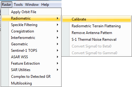
Выбор пункта меню Calibrate
Исходный продукт должен быть вновь созданным подмножеством. Результирующим продуктом будет новый файл, который вы создадите. Также необходимо выбрать каталог, в котором результирующий продукт будет сохранен.
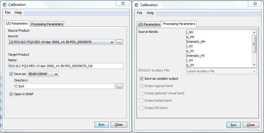
Диалог инструмента калибровки
Если вы не выберете какой-либо канал, то оператор калибровки автоматически выберет все реальные и мнимые (i, q) каналы. Снимите флажок «Сохранить в комплексе», чтобы оператор смог производить калибровку единого Sigma0-канала для реальной и мнимой пары. Вам необходимо откалибровать и хранить данные как комплексное значение в случае выполнения поляриметрической обработки.
[править] Некогерентное накопление (multilooking)
Некогерентное накопление (multilooking) может быть использовано для получения продукта с условным размером пикселей изображения.
Некогерентное накопление может быть сформировано путем усреднения разрешения пикселов по дальности и/или по азимуту, повышая радиометрическое разрешение, но ухудшая пространственное разрешение.
В результате, изображение содержит меньше шума и приблизительное квадратный размер пикселя после преобразования от наклонной дальности к дальности до поверхности земли.
Некогерентное накопление является необязательным этапом, поскольку оно не требуется, когда изображения корректируется по местности.

Некогерентное накопление (multilooking) SLC продукта
Шаг 3 — Некогерентное накопление канала Intensity_VH: Из меню Radar, выберите пункт Multilooking
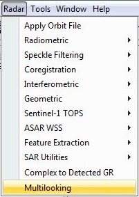
Выбор процедуры некогерентного накопления
В диалоге Multilook, выберете канал Intensity_VH для того, чтобы обрабатывать только его.
Укажите число видов по дальности, при этом число видов по азимуту будет вычислено на основе расстояния до земли и расстояния по азимуту.

Выбор канала Intensity_VH
Процедура некогерентного накопления создаст квадратный пиксель дальности до земли, используя 1 вид в дальности и 3 вида по азимуту. В результате средний размер пикселя дальности до земли будет 13.95 м.
Нажмите Run, чтобы начать обработку.
После завершения будет создан и доступен новый продукт в Product Explorer.
В новом продукте откройте канал Intensity_VH.

Результирующий канал Intensity_VH
Изображение выглядит более пропорционально, однако, оно по прежнему содержит большое количество шума.
[править] Фильтрация спекл-шума
Спекл вызван случайной конструктивной и деструктивной интерференцией, порождающей шум как «соль и перец» по всему изображению.
Спекл-фильтры могут быть применены к данным для уменьшения количества спекл-шума за счет размытия деталей или уменьшения разрешения.
Шаг 3 — Фильтрация спекл-шума: Выберите продукт с некогерентным накоплением, а затем выберите Speckle Filtering/Single Product Speckle Filter из меню Radar.

Выбор фильтрации спекл шума для единичного продукта
В диалоговом окне Speckle Filtering выберите спекл-фильтр Refined Lee. Фильтр Refined Lee усредняет изображение, сохраняя края.
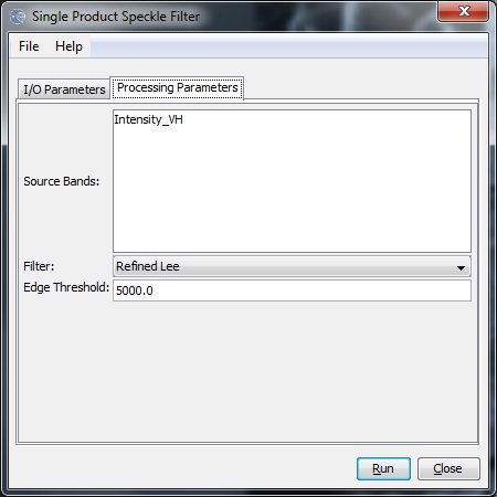
Диалог фильтрации спекл шума для единичного продукта
Нажмите Run для обработки.
Откройте вновь созданный продукт с отфильтрованным спекл-шумом.
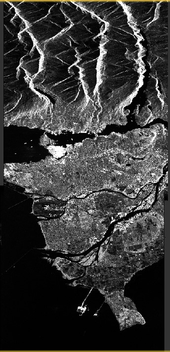
Результат использования спекл-фильтра
Заключительной обработкой, которую мы произведем над этим продуктом, будет корректировка по местности.
[править] Корректировка по местности
Корректировка по местности геокодирует изображение, исправляя геометрические искажения РСА с использованием цифровой модели высот (DEM) и производит продукт в картографической проекции.
Геокодирование корректирует изображение из геометрии наклонной дальности или расстояния до земли в картографическую систему координат. Геокодирование по местности включает в себя использование цифровой модели высот (DEM) для коррекции геометрических эффектов, присущих РСА, таких как эффект складки (foreshortening), переналожение (layover) и тени (shadow).
Эффект складки
- Период времени, в котором склон облучается передаваемым импульсом энергии радара, определяет длину уклона на радарном снимке.
- Это приводит к сокращению склона местности на радарном снимке во всех случаях за исключением, когда локальный угол склонения (θ) близок к 90°.
Переналожение
- Когда верхняя часть склона местности ближе к радарной платформе, чем нижняя, она будет записана раньше.
- Последовательность, в которой изображаются точки вдоль местности, производит изображение, которое получается перевернутым.
- Переналожение радара зависит от разницы в расстоянии наклонной дальности между верхней и нижней частями элемента.
Тени
- Задняя часть склона загораживается от отраженного луча, порождая отсутствие возвращаемой области, т.е. радарную тень.
Последствия этих искажений можно увидеть ниже. Расстояние между 1 и 2 могут оказаться короче, чем следует, и возврат для 4 может произойти до возврата для 3 из-за высоты.

Геометрические эффекты РСА
Шаг 4 — Корректировка по местности: Выберите продукт с некогерентным накоплением и спекл-фильтрованный продукт, а затем выберите Range-Doppler Terrain Correction из меню Radar/Geometric/Terrain Correction.
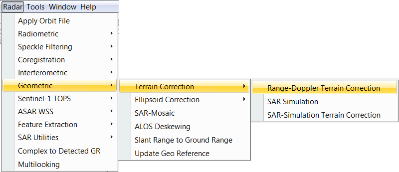
Выбор инструмента корректировки по местности
По умолчанию, для корректировки по местности используется SRTM 3-sec DEM. Программа автоматически определит необходимые тайлы DEM и скачает их автоматически с интернет-серверов.
Картографическая проекция по умолчанию — Географическая Широта/Долгота.
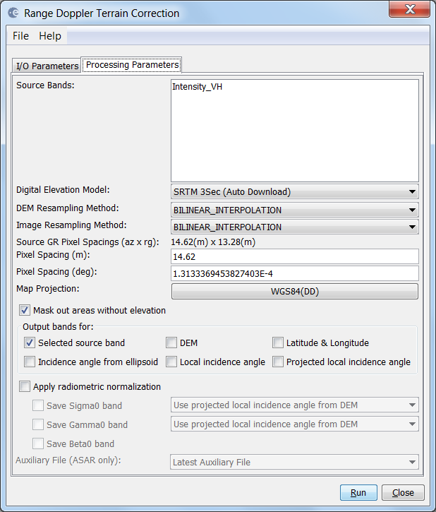
Диалог корректировки по местности
Нажмите Run для обработки.
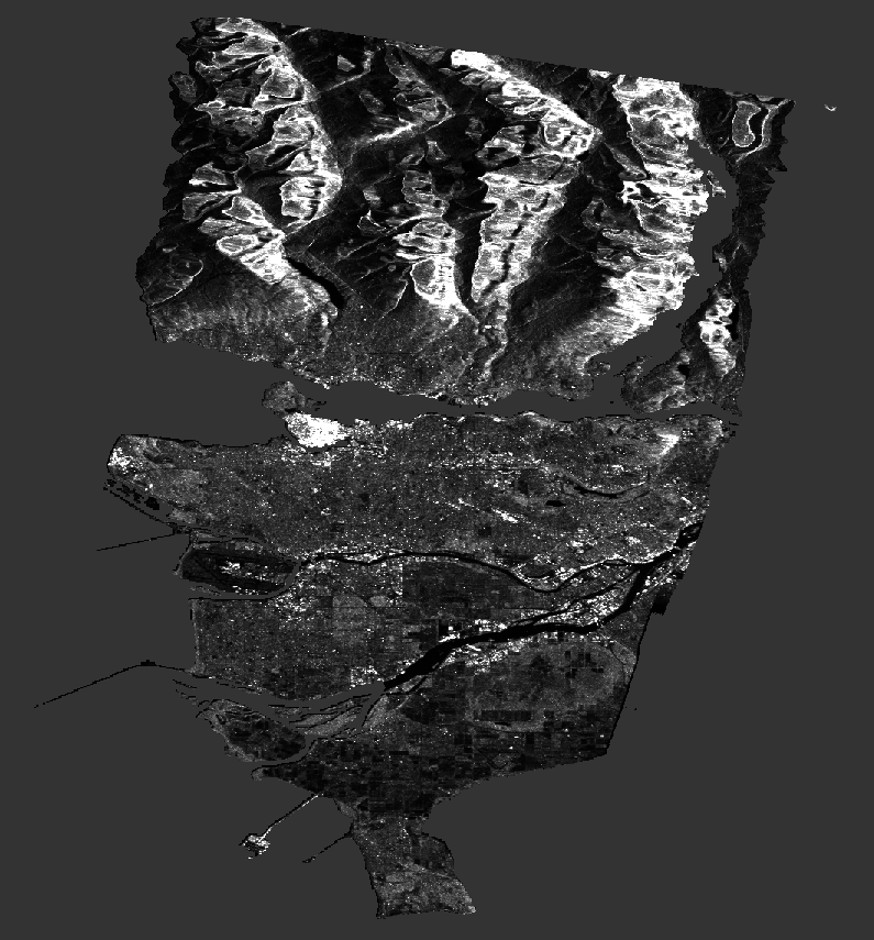
Откорректированное по местности изображение
Для просмотра изображения в шкале децибелов кликните правой кнопкой мыши на скорректированный по местности канал Intensity_VH и выберите Linear to/from dB для конвертации данных, используя виртуальный канал.
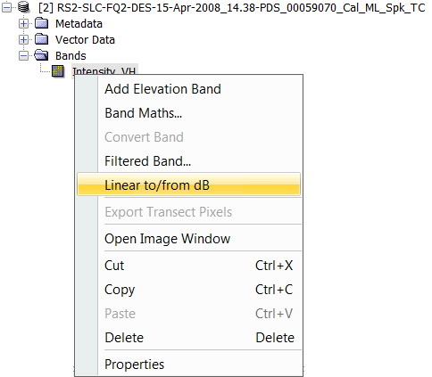
Выбор Linear to/from dB
Будет создан новый канал, основанный на выражении 10*log10(Intensity_VH)

Новый канал Intensity_VH_dB
Дважды кликните на канале Intensity_VH_dB для того, чтобы открыть его.
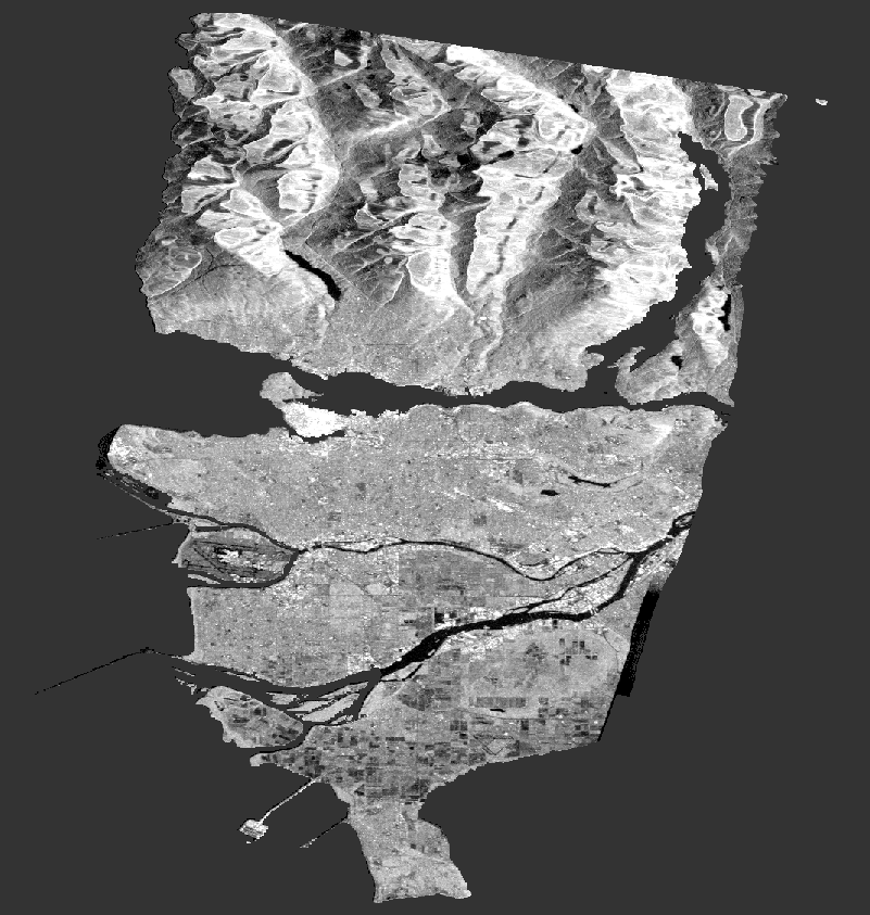
Откорректированный по местности канал в децибелах
I was about to write a post on preprocessing Sentinel 2 data using SNAP, similar in tone to the previous one on Sentinel 1, when I realized that most of the things I was about to say are already well explained in an excellent video produced by ESA. So, we will keep the topic very short here.
In our previous post, we have already reviewed how to download data. We here show how to explore them with ESA’s SNAP tool. First, get the latest version of SNAP. In my case, I still had the same old version that I used to write the post on Sentinel 1, and that one did not work right away with Sentinel 2. So, check here and get the latest version of SNAP and the Sentinel toolbox. The data files are opened by pointing to the xml file inside the folder:

In this example we did not open the whole file, but just one of the tiles inside the “GRANULE” folder. In this case, “T33TVF” corresponding to the Vesuvius area, at the Bay of Naples, Italy. Alternatively, one might also directly access the image files inside the folder IMG_DATA, which are already rectified and projected in the corresponding UTM zones. Images are coded in 16 bit unsigned integers, with scales and offsets for all 13 bands available in the metadata for calculating radiances. The data even includes rasters for sun azimuth and elevation, which are needed for calculation of reflectance:

The images are of great quality and, at 10 m pixel size, the views are really impressive:

and even more in detail:


The MSI instrument has the unique feature of offering three bands (5, 6 and 7) specifically designed to capture the vegetation ramp, which is extremely useful for vegetation studies. Otherwise, bands 8, 4, 3 and 2 (NIR, R, G and B) closely match bands 5, 4, 3 and 2 of Landsat 8 OLI, which offers the opportunity of using Sentinel 2 MSI and Landsat 8 OLI images as complementary instruments. See, for example, this post describing a comparison of spectral responses of Landsat and Sentinel instruments.
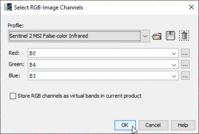
Creating the RGB color images in SNAP is easy. Just click on the “Window” tab and choose “Open RGB Image Window”, a simple menu will open that will allow you to choose the combination you need (natural color, and IR color are preprogrammed):

Finally, one of the interesting gems in SNAP is the “Spectrum View” tool, found under the “Optical” tab, which builds spectral plots of the image at the location of the mouse pointer:

Happy working with Sentinel 2 data!
From AWF-Wiki
Jump to: navigation,
search
Contents
- 1 Reading a Sentinel-2 tile
- 2 Displaying a Sentinel-2 tile
- 3 Resampling
- 4 Subsetting
- 5 Write to permanent file
Reading a Sentinel-2 tile
- Download a complete Sentinel-2 tile from ESA Open Access Hub (see Downloading Sentinel-2 images).
- Start SNAP Desktop
- File —> Open Product… Browse to the compressed Sentinel-2 zip file. Open or drag and drop the zip file from Windows File Explorer into the SNAP Product Explorer tab.
- Click on the plus sign of the file name in Product Explorer. Unfold Metadata and Bands.
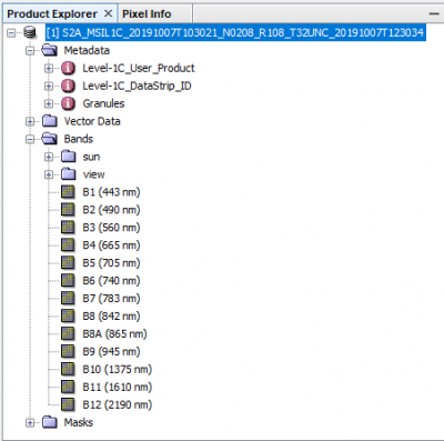
Displaying a Sentinel-2 tile
- Mark the file name in the Product Explorer. Right click Open RGB Image Window). In the Profile drop-down list select Sentinel 2 MSI False Colour Infrared. OK
Resampling
The spatial resolution of all satellite bands should be resampled to a unique pixel size (10m) to simplify the processing workflow.
Raster —> Geometric —> Resampling. Open the Resampling Parameters tab. Define size of resampled product: check by reference band from source product. Select B2 from drop down list. Run.
Subsetting
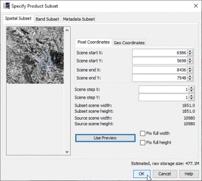
Spatial subset
- Mark the file name of the resampled product from previous work step in Product Explorer.
- Raster —> Subset..
- Left click in the preview of the Specify product subset dialog.
- In the Spatial Subset tab draw a box on top of the preview image and move it to your region of interest.
- Make a note of Pixel Coordinates and (Geographical)’ Geo Coordinates if you want to repeat this step with other acquisiton dates of the same tile.
Spectral subset
- In Band Subset tab click Select none and then check only the multispectral Reflectance Bands (B2,B3,B4,B5,B6,B7,B8,B8A,B11,B12). OK.

Write to permanent file
Mark the subset file name in Product Explorer.
File —> Export —> GeoTIFF. Click Export Product.
forward from:
08-SNAP command line processing tool GPT and its batch (Sentinel-1 and Sentinel-2 as an example)
- Introduction
- Foreword
- GPT command line tool introduction
-
- GPT command line tool
- GPT command line syntax parameters
- data source
-
- Sentinel-1 data
- Sentinel-2 data
- GPT implementation single operation
-
- Single data set single operation processing
-
- SENTINEL-2 NDVI calculation
- Sentinel-1 Track Correction
- Multiple data set batch single operation processing
-
- Sentinel-2 timing NDVI calculation
- Sentinel-1 batches of orbit correction
- GPT matching flow chart implementation process processing
-
- Single data set flow chart processing
-
- SENTINEL-2 L2A Data Flow Process Process
-
- Save flow chart file
- SENTINEL-1 IW GRDH Dataset Process Process
- Multiple data set batch flow chart processing
-
- SENTINEL-2 L2A Data Set Batch Process Process
- Sentinel-1 IW GRDH Dataset Batch Process Processing
- Whim
- references
Introduction
If I tell you, I only need a line of code in SNAP to complete the pretreatment of SENTINEL satellite images throughout the year, but only take hours, do you have Snap this «scraping»?
Foreword
Hemisted Snap GUI (Graphical User Interface) interface often complains that SNAP is slow, the processing speed is slow, there is no GPU acceleration function, and these already have many users in the SNAP official forum, Snap official developers have started to start solve these problems. The main reason is that the source code of SNAP is written by Java, relative to C / C ++ and other compilation languages, and the speed is slower when the large data is calculated, and the other problem is that the Java virtual machine is often in SNAP. The memory cannot be released in time, resulting in the processing or error of large data volume or very slow. Of course, there is a significant benefit using Java, that is, the cross-platform (Windows, Linux, UNIX, MAC systems) is running, which is greatly developed. Displaying slow reasons, I think it should be Snap to save image data, unlike ENVI, ArcGIS has not created the corresponding image pyramid assistance file, and if the pyramid is created, there will be a lot of hard disk space, in short, there is always some advantages.
However, it is not to say that there is no way to speed up the running speed of SNAP.On the hardware, the big running memory is clearly accelerated to accelerate the processing of large data volume images, and the solid-state hard drive significantly improve the read and write speed of video data, these are general hardware acceleration methods, but it takes a certain fee; software, use SNAP flowchart or command line tool GPT can significantly accelerate data processing speed, which is the way I have been advocating Snap to handle Sentinel satellite images because it avoids the data read and write process of a large number of intermediate processes. Of course, the GPT tool is already compiled after compiled binary programs (like a C / C ++ et al. Like the .exe executable program), not the Java virtual machine recognizes the JAR program (Java bytecode program), which has a certain speed Improvement. Of course, SNAP’s Python package snappy or uses Java source code combined with multi-process, multi-thread technology, and blocking techniques in parallel computing are also an acceleration method.
This time, discussing the SNAP command line tool GPT, next, you can see the leap to use the GPT tool to bring the quality of the data processing, and this is only a small amount (a sentence or a few words). Data processing can be completed efficiently. Here, I would like to thank the Snap official developer’s excellent design of the command line tool, so that we can easily achieve fast pretreatment of SENTINEL and other satellites and conventional remote sensing processing.
Although this paper is an example of a Windows10 system, the GPT tool command using SNAP in Linux, the Mac system is similar.
(The blogger has recently purchased two 16G memory strips (about 400 yuan per one), will run memory upgrade to 32G (previously 16g), and condition can be used to buy a memory strip upgrade in connection with the actual situation of the computer, in the SNAP The experience should be greatly improved. However, in addition to the batch processing of the text, small memory computer (4G or 8G) may have an error in memory, some simple GPT command line operations should be no pressure.This article, except for the last Sentinel-1 IWGRDH batch processing operation requires high storage (should require 16G memory), the rest should be 8G memory. Don’t necessarily be like bloggers, not to reach 32G. However, big running memory, relatively, handling big data is convenient! In addition, you should ensure that the C disk has at least 20G space to store a large number of temporary files generated by Snap or GPT operations)
GPT command line tool introduction
Although you can use the Snap GUI interface, you can do not write the code. You can do numerous processing operations through the click of the mouse, however, once you are familiar with the SNAP GPT tool, process SENTINEL satellite data will be very mindful, just like «tat melon cooking» Natural, simple. Some interfaces that do not have a command line, which may be dark, which may feel fear, in fact, the early computer is only such a command line interface (including the current Linux, Mac system to remain like this), this only returned to comparative original On the programming interface, writing programs with ordinary IDE interface is basically the same, except for grammar. In fact, start the GUI interface, take up a lot of system resources, and the running speed of slowing down in the system is limited. Fortunately, we only need to master the minority SNAP’s GPT command line tool command to complete the most processing. Ok, talk so much, is it like this, I need to experience it!
The GPT command line tool (GPT.exe) is located under the bin folder under the SNAP folder (under the same folder in the same folder) under the SNAP installation path (under the same folder), as follows is the blocker installation path:E:SNAPinstall_pathsnapbin
As shown below:
If you can’t see the suffix name .exe, you may need to set up a file extension and hidden items:
In the above figure, you can see multiple .exe programs (and corresponding profile .vmoptions), where snap64.exe is the main program of starting the Snap GUI interface, and PConvert.exe is a data conversion program. If you enter: Snap64 in the command line, you will find that the Snap GUI will start (actually, the SNAP desktop shortcut is binding is this program).
Start the command line interface under the current file path:
Or press the SHIFT button + mouse button:
Enter: SNAP64 (or Snap64.exe), you will find that the SNAP’s GUI interface is open.
To avoid the Calling GPT is not used to start the command line interface under the SNAP installation path, it is recommended that you add the BIN folder under the SNAP installation path to the BIN folder in the SNAP folder to the user environment variable:
GPT command line syntax parameters
Enter the command line interface on the open:
gpt -h
- 1
(You may need to wait for more noct, because this command line includes the operation and command, will show a large English document description, the mouse is pulled forward, first look at the front parameters. Under the case, We don’t remember so much parameters, just find it when you use it)
It can be seen that its syntax description (USAGE), the angle-in-axis <> indicates the parameters that must be filled in, and the bucket [] represents an optional parameter, vertical line |: Used to separate multiple mutual exclusion parameters, meaning «or», You can only select one when used. If you want to see the common syntax format of the command line, you can see this blog.Command line grammar format and special characters。
# <op> Represents a certain operator, <graph-file> represents the SNAP flow chart file (XML file); see the arguments parameter
 # <options> Represents optional parameters, -H, -E, -F, etc. See options options
 # <source-file-1> Indicates the source data file, of course, multiple source data files can be
gpt <op>|<graph-file> [options] [<source-file-1> <source-file-2> ...]
- 1
- 2
- 3
- 4
(# ) is an annotation description)
There are several Options parameters to be more important.You may temporarily do not understand the description of the -s and -p parameters, but it is not important. With doubt, continue to look down, then show its usage, then discuss the meaning of it):
- -h: Display help command;
- -t <file>: Indicates the output file name (represented by file), if this parameter is not, the default output file name is Target.dim;
- -f <format>: Indicates the format of the output (represented by format), the default is «beam-dimap», of course, you can also enter «geotiff», «envi» and other formats;
- -S<source>=<file>: This is the source file parameter variable defined by the XML file $ {<source>} indication (whose -s? Answer is short, s represents the first letter of SOURCE).
- -P<name>=<value>: This parameter and -s <source> = <value> are similar, but more universal, you can set name the word value to variables in the XML file (whose -p? Answer is also short, P Represents Parameters of the first letter) . The rear batch is to show its usage;
If you continue to pull down, you can see Opterators, which is the following: Snap supported (in order to arrange, A-> Z):
data source
Sentinel-1 data
To cover the Sentinel-1 IW GRDH product data of Shanghai (June 19, 2019) Tried an example (source data no need to decompress):
The range is as follows:
Sentinel-2 data
Taking the Yellow River Delta region where it is located in Dongying City, Shandong Province is an example.
The range is as follows:
GPT implementation single operation
Single data set single operation processing
SENTINEL-2 NDVI calculation
In the parameter table of the GPT command line parameter interface Operators, the NDVIOP operation started to the beginning of the N letters, which is the SNAP’s NDVI calculation command line operation we have to find, under the command line interface, enter: GPT NDVIOP -H, You can view the description of the operator command parameter (GPT, NDVIOP can be mixed, but the parameters of the belt — the parameters need to be strictly sized, such as here -h).
gpt NdviOp -h
- 1
You can see the following parameters description:
Source file parameters-Ssource=<file>Representing the source data, the file name of File is replaced, and the angle brackets indicate that the parameter is necessary, can not be missing, the back float, string’s sharp brackets also means the same meaning;
-PnirFactor=<float>,-PredFactor=<float>The proportional modulation factor of the near infrared band, the red light band is respectively, and the proportional factor is 1 in our common NDVI, and the default value is 1.0F (1.0 indicating the floating point number), usually we do not need to enter this parameter;
-PnirSourceBand=<string> , -PredSourceBand=<string>Indicates the near infrared band, the red light wave section, and String represents the wave section;
Thereafter, there is aGraph XML FormatDisplay the XML file content that is called by default, here you see $ {source} in the <sourceES> node, so the parameters for our source file are -ssource = <file>. If I use the <source code} to $ {INPUT} in the XM file I use, then we transfer to the source file, then the source file parameter is changed to -Sinput = <file>. Here, there should be a default XML file for the time being, temporarily put on holding a change in a while.
The command of this operation is available for usage:
# Optional Represents optional parameters, the above - related parameters, such as -ssource, etc.
gpt NdviOp [optional]
- 1
- 2

Simply display, blog’s source data folder and output folder location:
Take the first scene data as an example, that is, S2A_MSIL2A_20190122T025021_N0211_R132_T50SPG_20190122T065329.Zip
Ok, it is time to show its command line method (note = no spaces on both sides, the -t parameter is not equal, input and saved file path may need you to manually modify, the output file name is S2A_MSIL2A_20190122T025021_N0211_R132_T50SPG_2019012222222229_ndvi.dim, Plus the suffix and use the standard SNAP format beam-dimap if the suffix name is changed to .tif, the default is output in «geotiff» format, of course, on the command line, plus -f «geotiff»).
# Although it is a command, it is very long after adding a path. You can copy the last line command to a .txt file,
 # Easy to edit the command in .txt text. After confirming that the command is correct,
 # Open the command line interface (click on the mouse in the command line interface, you can paste the copy of the copy)
 # -Ssource indicates the absolute path of the source file (although the relative path can also be used, the absolute path is safe),
 # Why add a double quotation number in the path, which avoids the path in the path to cause the path to be separated.
 # -PnirsourceBand indicates near infrared wave paragraph name, and the near-infrared band corresponding to Sentinel-2 is named B8.
 # -PredsourceBand indicates that the red light wave segment name is named B4, and the red light wave section name is b4.
 # B8 and B4 resolution are 10m, and the grid image size is the same, so the calculation of NDVI can be performed.
 # -t indicates the file name of the output, the path is also added to the double quotes, pay attention to the bloggers, plus the suffix _NDVI.DIM
gpt NdviOp -Ssource="G:2019_S2_dataS2A_MSIL2A_20190122T025021_N0211_R132_T50SPG_20190122T065329.zip" -PnirSourceBand="B8"  -PredSourceBand="B4" -t "G:2019_S2_dataTest_NDVIS2A_MSIL2A_20190122T025021_N0211_R132_T50SPG_20190122T065329_ndvi.dim"
- 1
- 2
- 3
- 4
- 5
- 6
- 7
- 8
- 9
- 10
(Looking for a command to take a few times, the command to calculate the NDVI is about two minutes, speed is still possible)
Since the blogger has added a BIN folder under the SNAP installation path to the environment variable, I can open the command line window in any of the folders, here is input
We import the original data (.zip), and generate the corresponding NDVI into the SNAP View Effect:
Perfect! You can call the NDVI tool in the SNAP command line interface to calculate, and the result should be the same.
(Of course, only dealing with a single data set and a single operation does not show the advantage of GPT, or even you need to record so many command line parameters, showing the power of its power, more reflected in the batch, keep a little patience Continue to see it down)
Sentinel-1 Track Correction
In fact, the use of radiation calibration operation is better, but the track correction is usually the first step in SAR data processing in SNAP, and it is also possible to demonstrate only Sentinel-1 GPT single operation command line processing.
You can pass the command line command:
gpt -h
- 1
Locate the track calibration Operator command name: Apply-Orbit-File (if you are familiar with the SNAP GUI interface is very known)
Next: Usage of this command:
gpt Apply-Orbit-File -h
- 1
You can see its usage and parameters (note that the three -pxxx parameters under Parameter Options have default, we can use it in the command line command):
Of course, its default parameter settings and SNAP’s GUI interface default parameters are one or one (In SNAP, each GUI operation interface can view its corresponding XML file parameters):
Open the SNAP GUI interface (which can be imported into Sentinel-1 data, or does not import it), click Radar-> Apply Orbit File, you can open the GUI interface of this action.
Then click File-> Display Parameters …
View the parameters (can be compared with the command line Apply-ORBIT-File.It can be seen that the default values of their parameters are the same, and the parameter name is also the same, in addition to the command line parameters to bring -P word. As mentioned earlier, P is the first letter of parameters:
Here is the Sentinel-1 IW GRDH data as an example:
S1A_IW_GRDH_1SDV_20190617T095445_20190617T095510_027718_0320F1_218D.zip
Ok, it’s time to show it. Since we use the default parameters, this is simple to calculate the NDVI command, this is simple (note = no spaces on both sides, the -t parameter is no equivalent, the input and saved file path may need you to modify it, The output file here is S1A_IW_GRDH_1SDV_20190617T095445_20190617T095445_20190617T095445_20190617T095445_20190617T095510_027718_0320F1_218D_ORT.DIM, plus a suffix and use a standard SNAP format beam-dimap, if the suffix name is changed to .tif, the default is output in «geotiff» format, of course, on the command line, plus- f «geotiff»).
# Although it is a command, it is very long after adding a path. You can copy the last line command to a .txt file,
 # Easy to edit the command in .txt text. After confirming that the command is correct,
 # Open the command line interface (click on the mouse in the command line interface, you can paste the copy of the copy)
 # -Ssource indicates the absolute path of the source file (although the relative path can also be used, the absolute path is safe),
 # Why add a double quotation number in the path, which avoids the path in the path to cause the path to be separated.
# -t indicates the file name of the output, the path is also added to the double quotation mark, pay attention to the bloggers to join the suffix _orb.dim
gpt Apply-Orbit-File -Ssource="D:temp_SARS1A_IW_GRDH_1SDV_20190617T095445_20190617T095510_027718_0320F1_218D.zip" -t "D:temp_SARtest_apply_orbit_fileS1A_IW_GRDH_1SDV_20190617T095445_20190617T095510_027718_0320F1_218D_Orb.dim"
- 1
- 2
- 3
- 4
- 5
- 6
- 7
Run the result (about one or two minutes):
Import the original data and the track correction data into the results correctly or not: Perfect! correct. Ok, then tell the batch of a single operation.
Multiple data set batch single operation processing
(When processing, make sure your hard disk has enough storage space, download the dataset to place it separately under a folder, do not use the Chinese path.)
Sentinel-2 timing NDVI calculation
If you have multiple Sentinel-2 video data in a certain area, you should want to get its timing NDVI curve, which may be vegetation, crops, etc. Classification or monitor common timing characteristic curves, which may be Sentinel-2 more The most common demand is analyzed. However, this demand is easy to achieve with Snap’s GPT command line tool. I have downloaded the Monthly Sentinel-2 L2A image of the Yellow River Delta 2019, just need to be used in the GPT command line to implement bulk NDVI calculations (execute NDVIOP operators).
Note PowerShell (this is a command line similar to the Linux terminal, but the syntax is not complete and the Linux) and the Windows standard command line command. The following syntax should be run in the standard command line. Fortunately, it is easy to enter the Windows standard command line window at the PowerShell command line window, just enter CMD on the PowerShell command line window (which is a prompt with PS):
cmd
- 1
The blogger’s data is placed under this folder (G: 2019_s2_data), the output directory is g: 2019_s2_data test_ndvi (although the last single data set NDVI operation result, the batch does not affect, default Will cover the data set, of course, you can also manually delete it):

Start PowerShell in the input file directory, then enter CMD, switch to the command line window of the Windows standard:
Then enter the last order below (see the execution interface above):
(If you need to handle your own data set, just modify the corresponding input, output the directory path)
# Although it is still a command, it is very long after the path is added. You can copy the last line command to a .txt file,
 # Easy to edit the command in .txt text. After confirming that the command is correct,
 # Open the command line interface (click on the mouse in the command line interface, you can paste the copy of the copy)
 # / r "g:  2019_s2_data" means it iteration file under the path, this is the directory of the blog
 #% X is an iterative variable, which is used to represent an iterative zip file absolute path.
 # * .zip is the regular expression syntax, which is the suffix contains .zip file
 # -Ssource =% x Represents source file for GPT
 # -t "g:  2019_s2_data  test_ndvi % ~ nx_ndvi.dim" indicates the full absolute path of the output file.
 # G:  2019_s2_data  test_ndvi is the output file path of the blogger,
 #% ~ NX means that the XXXX.zip file does not have the file name of the suffix .zip.
 #
for /r "G:2019_S2_data" %X in (*.zip) do (gpt NdviOp -Ssource=%X -PnirSourceBand="B8"  -PredSourceBand="B4" -t "G:2019_S2_dataTest_NDVI%~nX_ndvi.dim")
- 1
- 2
- 3
- 4
- 5
- 6
- 7
- 8
- 9
- 10
- 11
- 12
(If you don’t know very well for the Windows command line for loop command, you can refer to this articleBAT batch script tutorial (detailed script home supplement))
In addition, I want to prove that the SNAP’s GPT command line is high, a simple way, is that you can open the task monitor to see its CPU utilization (if you are interested, you can perform comparison with the Snap GUI interface):
It takes about 10 minutes (12 view images, and the average is less than one minute):
To the output data directory:
well! All I want is all.
Of course, the NDVI image of the Yellow River Delta 2019 we already have, next to see how to view a point in the Snap GUI interface (usually you can do your measurement point, if you have the latitude and longitude coordinate of the latitude) curve:
Import data first:
Open a scenic ndvi image:
Before this, first answered a question: According to the same footprint (according to the Copernic Data Center, or you are also a research area is also possible) Do you need a registration? The answer is not required, because the Co-2 images have been produced by Sentinel-2 images in the production of SENTINEL-2 images (using them closely over the global control point, adjustment and control error geometric error), Of course, if you measure a wide range of control points, you can ensure the accuracy of the measurement, you can also make a registration. If it is the SENTINEL-2 (S2A, S2B, single source) source image of the same study area (the same footprint), it is not necessary, but if it is a different source of data, such as Sentinel-2 and Landsat, Sentinel- 1 and SENTINEL-2, if different source data is fuse, it is best to register.
In order to let you see the geometric correction (positive shot correction) effect of Sentinel-2 images, you can use the former four view NDVI images, and the uniform split screen is displayed (and I can tell you, even video size, grid pixels are consistent ):
Uniform screen:

If you compare the light-produced satellite data, you will be amazed at the geometric correction of Sentinel-2 data.
Very good, our Sentinel-2 NDVI dataset corresponds to one or one, then you can see its timing curve.
(3 NDVI video window that can be opened)
Open the timing curve window (see below):
Timing curve settings window:
(Although you can adjust the order in the data set by up or down arrow, the period is arranged in order, but this is not necessary for the timing curve window, the timing curve window automatically extracts the date and draws the time corresponding to the time. Sequence curve)
Screening the drawing band (here the ndvi_flag is not very useful for us, it is a logo band, measure NDVI quality, see04 blog)

For more details, please see Snap Official ForumTime Series (Temporal) of NDVIdiscussion.
Sentinel-1 batches of orbit correction
With the above experience, Sentinel-1 IW GRDH bulk track correction is also easy.
The Sentinel-1 source data set of the blogger is D: TEMP_SAR, the output directory is D: TEMP_SAR TEST_APPLY_ORBIT_FILE:
Batch calibration command:
(If you need to handle your own data set, just modify the corresponding input, output the directory path)
# Although it is still a command, it is very long after the path is added. You can copy the last line command to a .txt file,
 # Easy to edit the command in .txt text. After confirming that the command is correct,
 # Open the command line interface (click on the mouse in the command line interface, you can paste the copy of the copy)
 # / r "d:  TEMP_SAR" indicates that it iterates the file under the path, which is the directory of the blog source data.
 #% X is an iterative variable, which is used to represent an iterative zip file absolute path.
 # * .zip is the regular expression syntax, which is the suffix contains .zip file
 # -Ssource =% x Represents source file for GPT
 # -t "d:  TEMP_SAR  TEST_APPLY_ORBIT_FILE % ~ nx_orb.dim" indicates the full absolute path of the output file.
 # D:  TEMP_SAR  TEST_APPLY_ORBIT_FILE is the blog output file path,
 #% ~ NX means that the XXXX.zip file does not have the file name of the suffix .zip.
 #                     _ORB.DIM
for /r "D:temp_SAR" %X in (*.zip) do (gpt Apply-Orbit-File -Ssource=%X  -t "D:temp_SARtest_apply_orbit_file%~nX_Orb.dim")
- 1
- 2
- 3
- 4
- 5
- 6
- 7
- 8
- 9
- 10
- 11
- 12

At the end (about 1 minute and a half, 24 passengers need 40 minutes):

The processing of a single operation is not very useful for Sentinel-1. Sentinel-1 (or other SAR data) pretreatment often requires multiple steps (like flowchart processing operations).
GPT matching flow chart implementation process processing
If only a single processing operation is performed only in the GPT, it will not be a bit «small use», and the efficient processing of GPT can be reflected in process operations.
The flowchart documents used in this blog and the code are shown in Baidu cloud tray:
link:
Extraction code: EAK9
Single data set flow chart processing
SENTINEL-2 L2A Data Flow Process Process
Still in S2A_MSIL2A_20190122T025021_N0211_R132_T50SPG_20190122T065329.Zip
This scenic data is an example.
Create a Sentinel-2 L2A for classification feature datasets, the flow is as follows (if you are not very familiar with the steps of the flowchart, you can see04 blogBand overlay part):
This flow chart (creation flow chart must pay attention to the order of steps, otherwise it is easy to make an error) is actually a summary of the blog 03 and 04 blogs. Specifically, the Sentinel-2 data is resumed to 10 meters (in 10 m band 2) Based on the resolution), then cut out the Yellow River Delta area, then do the main component transform (extract 3 main components), and calculate the four texture characteristics (contrast, second-order angle) by obtaining the first main component through its common texture matrix. , Entropy, variance); calculate NDVI (normalized vegetation index), MNDWI (improved normalized water index), BI (soil brightness index), NDRE1 (redoublelling index), NDRE1 (redoublelling index), NDRE1 (Red Side Band Nature Index 1) Features; Finally, the texture feature, index feature, and the original spectral feature are superimposed through the BandMerge tool, and write to the data set.
Each process node parameter (only the parameters you need to pay attention to:
Read:
Resample:
Subset:
PCA:
GLCM:
BandMaths:
BandMaths(2):
BandMaths(3):
BandMaths(4):
BandMerge:
Write:
(Blogger created a source data directory created a S2_FEATURES folder for saving the generated Sentinel-2 feature dataset)
Save flow chart file

Then turn off the flowchart window, turn off the SNAP, enter the saved flowchart XML file, view the flow chart file:
You can see its node content (if you are familiar with the HTML web file, you should be able to identify the contents of each node), first look at its content to enhance your understanding of the flow chart parameter file, do not change the content.
(After the mouse browsing up and down, you can turn off the XML file)
I tell you next, just enter a command to enter a command using the GPT naming line, you can execute the pre-processing of the scene data, start a PowerShell command line window:
# G:  2019_s2_data  Test_s2_features.xml is the absolute path of the flowchart file,
 # You may have changed the path in conjunction with your flow chart file.
 # Because we define the input and output of the data set when you create a flow chart
 # So here the command line parameter does not input and output parameters
gpt G:2019_S2_datatest_S2_features.xml
- 1
- 2
- 3
- 4
- 5
Sorry, the above complex flow chart calculation, bloggers use the GPT command line tool, only two minutes (less than a small time), complete the calculation (of course, bloggers cut the research area to approximately 1 / 10, there is a lot of data, but its efficiency is still very high): Generated data set:
Import this data into SNAP looks:
Perfect! This is so easy and pleasant to get a data set for classification.
If you want to use this data set to do a random forest classification, please refer to05 blog。
SENTINEL-1 IW GRDH Dataset Process Process
Still in 07, this scene data is true:
Created flow chart, please refer to the blog07 flow chart pretreatment sectionPre-treatment part:
The node parameters of the flowchart are the same as the path diagram parameters of the 07 flowchart pre-processing section:
Then turn off the flowchart window and SNAP.
The source data of the blogger and the saved flow chart file directory are D: TEMP_SAR, the output file directory to be saved is D: TEMP_SAR SENTINEL_1_PROCESSED.
Enter a PowerShell window in the source data file directory, enter the following command:
# D:  TEMP_SAR  S1_IW_GRD_PREPROCESS.XML is the absolute path of the flowchart file,
 # You may have changed the path in conjunction with your flow chart file.
 # Because we define the input and output of the data set when you create a flow chart
 # So here the command line parameter does not input and output parameters
gpt D:temp_SARS1_iw_grd_preprocess.xml
- 1
- 2
- 3
- 4
- 5

Probably takes about 10 or more minutes, and it is done.
Import the pre-processed data into SNAP to view the effect:
The GPT tool has been well completed!
Multiple data set batch flow chart processing
Most of the features in the SNAP can find its operand in the flowchart, including the third plugin added to the SNAP, and as long as the node operation with the flowchart is, it can be implemented in the SNAP’s GPT.
SENTINEL-2 L2A Data Set Batch Process Process
(I estimate the amount of computation, and 8G running the memory is a batch of this flow chart. Because the flowchart is made, the computer runs this batch of computer to run this batch.)
Sometimes we want to get a multi-view Sentinel-2 feature data set in the same area to analyze its timing characteristics or timing variations or multiple-time classification or change detection. Fortunately, we can easily implement data quantity batch processing using the flowchart file and the GPT command line tool.
Using the Sentinel-2 L2A data set process processing section, the created flowchart file and the GPT tool are easy to achieve batch processing of the multi-view Sentinel-2 feature dataset. However, we need to make some small modifications to the flowchart XML file:
First open the corresponding flowchart file:
We need to modify the files of the input and output nodes, set the GPT command line -P parameter variable:
For the <file> content for the input node <node id = «read»>:
by:
<file>G:2019_S2_dataS2A_MSIL2A_20190122T025021_N0211_R132_T50SPG_20190122T065329.zip</file>Change to:
<file>$input</file>
The GPT command line -P parameter variable, indicated by the US dollar $, INPUT is its variable name.
which is
For the output node <Node ID = «Read»> <file> content:
By<file>G:2019_S2_dataS2_featuresSubset_S2A_MSIL2A_20190122T025021_N0211_R132_T50SPG_20190122T065329_features.dim</file>Change to:
<file>$output</file>
The GPT command line -P parameter variable, indicated by the US dollar $, Output is its variable name.
which is:
(Although only the GPT command line tool -P parameter variable is only defined in the input file and output file variables, you can define the argument of the flowchart as the -p parameter variable with the US dollar $, for example, you can need to define output data. Resolution, select output band, coordinate system, etc.)
After completing the modifications of these two, turn off the XML file, start a PowerShell window in the source data directory:
Note that the batch will first enter the Windows standard command line window (first enter CMD)
Then enter the following command:
# You may need to combine the actual adjustment of your input directory and output directory
 # / r "g:  2019_s2_data" means iterative directory
 #% X indicates the iterative variable set, that is, an absolute path of a (.ziP) file name.
 # G:  2019_s2_data  Test_s2_features.xml The absolute path to the flowchart file to be processed
 # -Pinput =% x Where -pinput indicates the input variable (-P parameter variable) in the flowchart,% X represents the file name referenced
# -Poutput="G:2019_S2_dataS2_featuresSubset_%~nX_features.dim" ,
 # -Poutput indicates the Output variable in the flowchart (-P parameter variable), g:  2019_s2_data  s2_features indicates the parent directory of the output file
 # Subset_% ~ nx_features.dim takes out the suffix name of the file name .zip,
 # And add the prefix subset_, suffix _features.dim
for /r "G:2019_S2_data" %X in (*.zip) do (gpt G:2019_S2_datatest_S2_features.xml -Pinput=%X  -Poutput="G:2019_S2_dataS2_featuresSubset_%~nX_features.dim")
- 1
- 2
- 3
- 4
- 5
- 6
- 7
- 8
- 9
- 10

It takes about half an hour (12 scenic data), it is ok!
Open SNAP to check the data (very nice):
Sentinel-1 IW GRDH Dataset Batch Process Processing
(Since this is a need for two scents, Sentinel-1 IW GRDH is designed, it is high for running memory, I estimate that 8G running memory computer may be more effective, 16G running memory computer should be no problem.In addition, you need to make sure that the save the data directory has enough storage space, Sentinel-1 data is usually large, and the landscape behind the inlaid is about 5g)
Similarly, if you need to do the same processing on Sentinel-1 IW GRDH data, define the -p parameter variable of the input and output of the GPT command line tool (of course, there can be other -p parameter variables).
This way, the flow chart of this blogger07 Blog Method 3: TOPSAR Technology MosaicThis flowchart is more complicated, as follows:
(There are two inputs, 1 output, the parameters of this flow chart07 Blog Method 3: TOPSAR Technology MosaicIt is no longer repeated here.
Because it is necessary to synthesize images of the entire Shanghai-range image by two scented Sentinel-1 IW GRDH images, it will bring trouble, how to ensure that the inlaid time is just right in bulk data. How old is the same as the other day?
However, if it is more troublesome in the command line, it is a bit troublesome to extract the file name information! I didn’t find the right cmd command, but it is true that the combination C language is undoubtedly achievable. In addition to this trouble, there may be a trouble, which is the problem that GPT’s occupation memory cannot be released in time, causing the program to slow or even report error.
Considering that you will introduce Snappy later, this batch process is achieved using Python calls CMD commands. There are many very convenient library bags in Python, we can use the standard library.About the memory release problem of GPT, one of the skills used here is killing processes, enforces memory of JVM (Java virtual machine). That is, once the CMD process is called, after executing the command, turn off the CMD process, and then start a CMD process process.
The idea is already, next. We need to modify the flowchart file (here the file name: s1_mosaic2.xml), define 3 -P parameter variables:
Node <read>:
by:
<file>G:testS1A_IW_GRDH_1SDV_20190828T095515_20190828T095540_028768_034210_860C.zip</file>
Change to:
<file>$input1</file>
The GPT command line -P parameter variable, indicated by the US dollar $, INPUT1 is its variable name.
Node <read (2)>:
by:
<file>G:testS1A_IW_GRDH_1SDV_20190828T095515_20190828T095540_028768_034210_860C.zip</file>
Change to:
<file>$input2</file>
The GPT command line -P parameter variable, indicated by the US dollar $, and INPUT2 is its variable name.
Before changing: After changing:
Node <Write>:
by:
<file>G:testS1A_IW_GRDH_1SDV_20190828T095515_20190828T095540_028768_034210_860C.zip</file>
Change to:
<file>$input2</file>
The GPT command line -P parameter variable, indicated by the US dollar $, and INPUT2 is its variable name.
Before changing:
After changing:
OK! Modified! All is ready except for the opportunity!
(The actual code is not long, the blogger adds a detailed note, it should be not difficult to understand.In addition, before this, be sure to check if there is enough storage space for the C drive.At least 20g should be 20g, should be in the previous GPT command line operation. The following code may also need to change the input, output path, and output files before, the suffix name)
# -*- coding: utf-8 -*-
 # Author: Super Wo Water
# Python 3.6.7 win64

 # Import Related Library
import os
import glob
import subprocess
import time


 # Sentinel-1 IW GDRH metadata compression package storage directory, enter the directory
data_path = r'D:temp_SAR'

 #  ,, sort the found metadata (.zip) according to the file name
 # This image of the same day is adjacent
datas = sorted(glob.glob(os.path.join(data_path, '*.zip')))

 #Flow chart file path
xml_file = r'D:temp_SARS1_mosaic2.xml'

 # Output Directory
output_path = r'D:temp_SARSentinel_1_processed'

 # #
 # Because the file name is sorted, you can determine the two view images of the same day, respectively.
part1_datas = datas[::2]
part2_datas = datas[1::2]


for input1, input2 in zip(part1_datas, part2_datas):
         # Get the file name of the input file
    basename_input1 = os.path.basename(input1)
         # Extract date time
    date = basename_input1.split('_')[4][:8]
         #
    print("date:", date)
         # The file name of the output, the suffix name '.dim' indicates the standard file format (beam-dimap) using SNAP (BEAM-DIMAP)
    out_file = 'S1_Shanghai_' + date + '.dim'
         #
    output = os.path.join(output_path, out_file)
         #     list
    command = ['gpt', xml_file, '-Pinput1=' + input1,
               '-Pinput2=' + input2, '-Poutput=' + output]

         # If you want to see the actual command line window command, you can cancel the comment for the following print statement
    #print(' '.join(command))

         # Call the CMD (Windows Standard Command Line Window) in a "killing process"
         #             "GPT XML_File -Pinput1 = INPUT1 -PINPUT2 = INPUT2 -POUTPUT = OUTPUT"
    subprocess.check_output(command)

         # "Take a refund" ---- Distributed reptile "philosophy", sleep 30s, waiting to release memory
         # Avoid GPT because the memory cannot be released in time, slow down program operation or cause an error
    time.sleep(30)
print("All done!")
- 1
- 2
- 3
- 4
- 5
- 6
- 7
- 8
- 9
- 10
- 11
- 12
- 13
- 14
- 15
- 16
- 17
- 18
- 19
- 20
- 21
- 22
- 23
- 24
- 25
- 26
- 27
- 28
- 29
- 30
- 31
- 32
- 33
- 34
- 35
- 36
- 37
- 38
- 39
- 40
- 41
- 42
- 43
- 44
- 45
- 46
- 47
- 48
- 49
- 50
- 51
- 52
- 53
- 54
- 55
- 56
Just do the program in Python (you should be able to hear the » » of your computer, because the Usage of the CPU is likely to soar to 100%, you must know the CPU core used by the GPT default call. How many of your computer is called, and how many cores are called.
The running interface in Pycharm (about 25 minutes of time gets a scene of the full-scale video, due to the large amount of data, you need to wait patiently):

You can finally get 12 scenery Shanghai Sentinel-1 IW GRD image (September 2019, Month, a monthly scene), a total of more than 5 hours:
Import Snap to see the result (here the 4 scenic VH channel is turned on):
OK! correct!
Similar to the previous Sentinel-2 NDVI timing curve, once we have multiple Sentinel-1 video data, we can also easily get its SAR back to the scattering coefficient time curve (I want to demonstrate the timing curve of 12 scenes, but compare Card, because the amount of data within the entire Shanghai has too much data, about 60g, 4 views here).
Prove that our operation is incorrect! See you!
Whim
I hope you can recognize the common usage of the SNAP’s GPT command line to efficiently complete the processing of the sentinel data. Although this article only introduces some basic operations, SNAP can do more. In fact, SNAP does the processing of many satellite data, is not only handling Sentinel series satellites (like landsat, modis, alos, envisat, etc.), just processing Sentinel satellite is its advantage.
Although this article does not mention more advanced processing techniques, such as multi-process, block processing, etc., these have retained their interfaces in SNAP, whether it is GPT or its python package snappy or Java source code can be realized, of course, Programming languages can also be implemented, but relatively, you need to do more work. The next item introduces some basic knowledge of SnapPy, maybe you can deepen some impressions!
Finally, if you are interested in the SNAP and its SNAPPY development processing software SNAP and its SNAPPY development process, you can join the Open Open Snap processing exchange group created by the blogger: 665903216 (this group is full of people), European SNAP processing group (2): 1102493346.
good luck!
references
[1] Snap Wiki Blog GPT Tool Batch Introductionhttps://senbox.atlassian.net/wiki/spaces/SNAP/pages/70503475/Bulk+Processing+with+GPT
[2] SNAP Command Line Tutoriall http://step.esa.int/docs/tutorials/SNAP_CommandLine_Tutorial.pdf
[3] Zhang Lei, Qiang Zhao Ning, Wang Qi, gold point, Wang Xing.Sentinel-2 video multi-characterized Yellow River Delta Wetland Information Extraction [J]. Remote Sensa, 2019,23 (02): 313-326.
[4] Li Peng, Li Di, Li Zhenhong, Wang Houjie. Research on GF-3 Radar Data and Sentinel-2 Multi-Spectral Data Wetland in the Yellow River Delta [J] .Journal of Wuhan University (Information Science Edition), 2019,44 (11): 1641-1649.