Webgl руководство по программированию - RukovodstvoRus.ru - инструкции пользования и руководства

Время на прочтение
13 мин

Количество просмотров 45K

Всем привет!

Хочу начать вольный перевод отличной книги «WebGL Beginner’s Guide», которая, на мой взгляд, будет интересна не только новичкам, но и более продвинутым разработчикам.

Содержание:

Глава 1: Начиная работать с WebGL
Глава 2: Рендеринг геометрии
Глава 3: Освещение
Глава 4: Камера
Глава 5: Движение
Глава 6: Цвет, глубина и альфа-смешение
Глава 7: Текстуры
Глава 8: Выбор
Глава 9: Собираем все вместе
Глава 10: Дополнительные методы

WebGL первоначально была основана на OpenGL ES 2.0 (ES означает Embedded Systems), версии спецификации OpenGL для таких устройств как iPhone от Apple и iPad. Но спецификация развивалась, стала независимой, ее основная цель это обеспечение переносимости между различными операционными системами и устройствами. Идея веб-интерфейса, рендеринг в реальном времени открыли новую вселенную возможностей для веб-3D сред, таких как видеоигры, научная и медицинская визуализация. Кроме того, из-за широкого распространения веб-браузеров, эти и другие виды 3D-приложений могут быть запущены на мобильных устройствах, таких как смартфоны и планшеты. Если вы хотите создать свою первую веб-видеоигру, 3D арт-проект для виртуальной галереи, визуализацию данных ваших экспериментов или любое другое 3D-приложение, вы должны иметь ввиду, что первым шагом должно быть то, что вы должны убедиться, что у вас есть подходящая среда.
В этой главе вы сможете:

Понять структуру WebGL-приложения
Создавать свои области рисования (canvas)
Проверить WebGL-возможности вашего браузера
Понять, как устроена машина состояний WebGL
Изменять переменные WebGL, которые влияют на вашу сцену
Загружать и исследовать полнофункциональные сцены

Системные требования

WebGL является веб-основой API 3D-графики. Как таковая она не требует установки. В то время, когда писалась это книга, вы автоматически могли работать с WebGL, если у вас установлен один из следующих интернет-браузеров:

Firefox 4.0 или более поздней версии
Google Chrome 11 или более поздней версии
Safari (OSX 10.6 или более поздней версии). По умолчанию WebGL отключена, но вы можете включить ее, установив опцию Enable WebGL в меню Developer
Opera 12 или более поздней версии

Чтобы получить обновленный список веб-браузеров, которые поддерживают WebGL, перейдите по следующей ссылке . Вы также должны убедиться, что на вашем компьютере имеется видеокарта. Если вы хотите быстро проверить, поддерживает ли ваша конфигурация WebGL, то перейдите по этой ссылке.

Что представляет собой WebGL

WebGL является 3D графической библиотекой, которая позволяет современным интернет-браузерам отрисовывать 3D-сцены стандартным и эффективным способом. Согласно Википедии, рендеринг это визуализация процесса создания изображения из модели с помощью компьютерной программы. Поскольку этот процесс выполняется на компьютере, существуют различные способы получения таких изображений.
Первое различие, которое мы должны сделать, используем ли мы какие-либо специальные графические аппаратные средства или нет. Мы можем говорить о программном рендеринге, в тех случаях, когда все расчеты, необходимые для отрисовки 3D-сцен выполняются с использованием основного процессора компьютера; с другой стороны, мы используем термин аппаратного рендеринга, в тех случаях, когда есть графический процессор (GPU) для вычисления 3D-графики в реальном времени. С технической точки зрения, аппаратный рендеринг является гораздо более эффективным по сравнению с программным, потому что есть специализированные аппаратные составляющие, которые обрабатывают операции. Но, с другой стороны, программный рендеринг обычно более распространен из-за нехватки аппаратных зависимостей.
Второе различие, которое мы можем сделать, это происходит ли процесс рендеринга локально или удаленно. Когда изображение, которое должно быть отображено сложное, то рендеринг, скорее всего, будет происходить удаленно. Это случай 3D-анимационных фильмов, когда выделенные серверы с большим количеством аппаратных ресурсов позволяют рендерить сложные сцены. Мы будем называть это серверным рендерингом. Противоположностью этому является рендеринг, выполняющийся локально. Мы будем называть это клиентским рендерингом.
WebGL имеет клиенто-ориентированный подход; элементы, которые составляют части 3D-сцены, обычно загружаются с сервера. Однако, вся дальнейшая обработка, необходимая для получения изображения выполняется локально, с помощью графического оборудования клиента.
По сравнению с другими технологиями (например, Java 3D, Flash и Unity Web Player Plugin) WebGL имеет ряд преимуществ:

JavaScript программирование: JavaScript это «родной» язык для веб-разработчиков и веб-браузеров. Работа с JavaScript позволяет получить доступ ко всем DOM-элементам, а также легко с ними обращаться, в отличие от общения с апплетами. Так как WebGL программируется в JavaScript, то это облегчает интеграцию WebGL-приложений с другими JavaScript – библиотеками, такими как JQuery и другими технологиями HTML5.
Автоматическое управление памятью: в отличие от своего собрата OpenGL и других технологий, где есть конкретные операции выделения и освобождения памяти вручную, в WebGL нет такой необходимости. Из этого следует, что при выходе JavaScript переменной из области видимости, память, занимаемая ей, автоматически освобождается. Это чрезвычайно облегчает программирование, уменьшает объем кода, делает его более ясным и понятным.
Проницаемость: благодаря современным технологическим достижениям, веб-браузеры с поддержкой JavaScript устанавливаются на смартфоны и планшетные устройства. На момент написания, Mozilla Foundation является программой для тестирования возможностей WebGL в телефонах Motorola и Samsung. Существуют подобные разработки поддержки WebGL для платформы Android.
Производительность: производительность приложений WebGL сопоставима с эквивалентными автономными приложениями (с некоторыми исключениями). Это происходит благодаря способности WebGL иметь доступ к локальным аппаратным ускорителям графики. До сих пор, многие веб-технологии для 3D рендеринга используют программный рендеринг.
Нулевая компиляция: учитывая, что WebGL написана на JavaScript, то нет необходимости в предварительной компиляции кода перед выполнением в веб-браузере. Это позволяет вносить изменения на лету и смотреть, как эти изменения влияют на 3D веб-приложение. Тем не менее, когда мы затронем тему шейдеров, то мы поймем, что нуждаемся в некоторой компиляции. Однако, это происходит с помощью наших графических аппаратных средств, а не в нашем браузере.

Структура WebGL приложения

Как и в любой библиотеке 3D-графики, в WebGL необходимо присутствие определенных компонентов для создания 3D-сцен. Эти основные элементы будут рассмотрены в первых четырех главах книги. Начиная с 5 главы, мы будем рассматривать элементы, которые не имеют отношения к работе с 3D-сценой, такие как цвета и текстуры, а затем, позже, мы перейдем к более сложным темам.
Элементы, к которым мы обращаемся, следующие:

Canvas: это заполнитель, где будет отображаться сцена. Это стандартный HTML5-элемент, который может быть доступен с помощью объектной модели документа (DOM) через JavaScript.
Объекты: это 3D сущности, которые составляют часть сцены. Эти сущности состоят из треугольников. Во второй главе мы увидим, как WebGL обрабатывает геометрию. Мы будем использовать WebGL-буферы для хранения многоугольников и увидим, как WebGL использует буферы для визуализации объектов на сцене.
Свет: ничего в 3D мире нельзя увидеть, если нет никаких источников света. Этот элемент любого WebGL-приложения будет рассмотрен в 3 главе. Мы узнаем, что WebGL использует шейдеры для моделирования света на сцене. Так же мы посмотрим, как 3D-объекты отражают и поглощают свет в соответствии с законами физики, а также обсудим иные модели света, которые мы можем создать в WebGL для визуализации наших объектов.
Камера: выступает в качестве холста для просмотра 3D-мира. Посмотрим, как с ее помощью можно исследовать 3D-сцену. В 4 главе, будут рассмотрены различные матричные операции, которые необходимы для получения перспективного вида. Также мы поймем, как эти операции могут моделировать поведение камеры.

Эта глава посвящена первому элементу нашего списка – canvas. В ближайших разделах мы увидим, как создать canvas (холст) и как настроить WebGL-контекст.

Создание HTML5 canvas

Давайте создадим веб-страницу и добавим HTML5 canvas. Canvas представляет собой прямоугольный элемент на веб-странице, где будет отображаться 3D-сцена.

Используя ваш любимый редактор, создайте веб-страницу со следующим содержимым:

	<!DOCTYPE html>
	<html>
		<head>
			<title> WebGL Beginner's Guide - Setting up the canvas </title>
			<style type="text/css">
				canvas {border: 2px dotted blue;}
			</style>
		</head>
		<body>
			<canvas id="canvas-element-id" width="800" height="600">
				Your browser does not support HTML5
			</canvas>
		</body>
	</html>

Сохраните файл как ch1_Canvas.html.
Откройте этот файл через поддерживаемый браузер.
Вы должны увидеть что-то похожее на это:

Что только что произошло?
Мы только что создали простую веб-страницу с содержащимся в ней холстом. Этот холст будет содержать наши 3D-приложения. Давайте разберем некоторые важные элементы, представленные в этом примере.
Определение CSS-стиля для границы
Это кусок кода, который определяет стиль холста:

<style type="text/css">
	canvas {border: 2px dotted blue;}
</style>

Как вы можете себе представить, этот код не является фундаментальным для создания WebGL-приложений. Тем не менее, синяя пунктирная линия является хорошим способом проверки, где находится холст, учитывая, что полотно будет изначально пусто.
Понимание атрибутов холста
В предыдущем примере есть 3 атрибута:

Id: это идентификатор холста в объектной модели документа (DOM)
Ширина и высота: эти два атрибута определяют размер нашего холста. Когда эти два атрибута отсутствуют Firefox, Chrome, и WebKit по умолчанию будут использовать холст 300×150.

Что делать, если canvas не поддерживается?
Если вы видите, что на экране появилось сообщение: Your browser does not support HTML5 (которое было записано между тегами и ), то вы должны убедиться, что используете браузер, который поддерживает WebGL.
Если вы используете Firefox и все еще видите сообщение HTML5 not supported, то проверьте, что включена поддержка WebGL. Для этого введите в адресной строке about:config, а затем посмотрите на свойство webgl.disabled. Если установлено в true то перейдите и поменяйте. При повторном запуске Firefox и загрузке ch1_Canvas.html вы должны увидеть пунктирные линии холста, то есть все в порядке.
При удаленном подключении, если вы не видите холст, то это может быть связано с тем, что Firefox внес в черный список некоторые драйверы графической карты. В этом случае ничего не остается, как использовать другой компьютер.

Доступ к контексту WebGL

Контекст WebGL это дескриптор (точнее, объект JavaScript), через который мы можем получить доступ ко всем функциям и атрибутам WebGL. Они составляют Application Program Interface WebGL (API).
Мы собираемся создать функцию JavaScript, которая будет проверять можно ли на холсте получить контекст WebGL. В отличие от других библиотек JavaScript, которые должны быть загружены и подключены в рабочий проект, WebGL уже находится в вашем браузере. Другими словами если вы используете один из поддерживаемых браузеров, то вам не нужно устанавливать и включать какую-либо библиотеку.
Мы собираемся изменить предыдущий пример, добавив JavaScript-функцию, которая будет проверять наличие поддержки WebGL в вашем браузере (пытаться получить дескриптор). Эта функция будет вызываться при загрузке страницы. Для этого мы будем использовать стандартное DOM-событие onLoad.

Открываем файл ch1_Canvas.html в вашем любимом текстовом редакторе (в идеале можно выбрать синтаксис для HTML/JavaScript).
Добавьте следующий код прямо под тегом

Мы должны вызвать эту функцию на событие onLoad. Измените содержимое тега body на следующее:

	<body onLoad ="getGLContext()">

Сохраните файл ch1_GL_Context.html.
Откройте файл ch1_GL_Context.html, используя один из браузеров, поддерживающих WebGL.
Если вы не сможете запустить WebGL, то увидите примерно следующее диалоговое окно:

Что же только что произошло?
Используя переменную JavaScript (gl), мы получили ссылку на контекст WebGL. Давайте вернемся и проверим код, который позволяет получить доступ к WebGL:

	var names = ["webgl", "experimental-webgl", "webkit-3d", "moz-webgl"];
	for (var i = 0; i < names.length; ++i) 
	{
		try 
		{
			gl = canvas.getContext(names[i]);
		} 
		catch(e) {}
		if (gl) 
			break;
	}

Метод холста getContext дает нам доступ к WebGL. Все, что нам нужно, это указать имя контекста, которое может быть разным у разных производителей. Поэтому мы сгруппировали все возможные имена контекста в массив names. Крайне важно проверить спецификацию WebGL (вы можете найти ее в интернете) на любые изменения, касающиеся соглашения об именовании.
getContext так же может обеспечить доступ к 2D-графике HTML5 при использовании 2D –библиотеки, в зависимости от имени контекста. В отличие от WebGL это соглашение об именах является стандартным. API 2D-графики HTML5 является полностью независимым от WebGL и выходит за рамки этой книги.

Машина состояний WebGL

Контекст WebGL может пониматься как машина состояний: как только вы измените любой из его атрибутов, то модификация сохранит свое состояние, пока вы снова не поменяете значение атрибута. В любой момент вы можете запросить состояние этих атрибутов, поэтому вы можете определить текущее состояние вашего WebGL-контекста. Давайте проанализируем это поведение на примере.
В этом примере мы собираемся научиться изменять цвет, который мы используем для очистки холста:

Используя ваш любимый текстовый редактор, откройте файл ch1_GL_Attributes.html:

	<html>
		<head>
			<title> 
				WebGL Beginner's Guide - Setting WebGL context attributes 
			</title>
			<style type="text/css">
				canvas {border: 2px dotted blue;}
			</style>
			<script>
				var gl = null;
				var c_width = 0;
				var c_height = 0;
				window.onkeydown = checkKey;
				function checkKey(ev)
				{
					switch(ev.keyCode)
					{
						case 49:
						{ 
							// 1
							gl.clearColor(0.3,0.7,0.2,1.0);
							clear(gl);
							break;
						}
						case 50:
						{
							 // 2
							gl.clearColor(0.3,0.2,0.7,1.0);
							clear(gl);
							break;
						}
						case 51:
						{ 
							// 3
							var color = gl.getParameter(gl.COLOR_CLEAR_VALUE);
							// Don't get confused with the following line. It 
							// basically rounds up the numbers to one decimal cipher 
							//just for visualization purposes
							alert('clearColor = (' + 
								Math.round(color[0]*10)/10 + 
								',' + Math.round(color[1]*10)/10+
								',' + Math.round(color[2]*10)/10+')');
							window.focus();
							break;
						}
					}
				}
				function getGLContext()
				{
					var canvas = document.getElementById("canvas-element-id");
					if (canvas == null)
					{
						alert("there is no canvas on this page");
						return;
					}
					var names = ["webgl", "experimental-webgl", "webkit-3d", "moz-webgl"];
					var ctx = null;
					for (var i = 0; i < names.length; ++i) 
					{
						try 
						{
							ctx = canvas.getContext(names[i]);
						} 
						catch(e) {}
						if (ctx) 
							break;
					}
					if (ctx == null)
					{
						alert("WebGL is not available");
					}
					else
					{
						return ctx;
					}
				}
				function clear(ctx)
				{
					ctx.clear(ctx.COLOR_BUFFER_BIT); 
					ctx.viewport(0, 0, c_width, c_height);
				}
				function initWebGL()
				{
					gl = getGLContext();
				}
			</script>
		</head>
		<body onLoad="initWebGL()">
			<canvas id="canvas-element-id" width="800" height="600">
				Your browser does not support the HTML5 canvas element.
			</canvas>
		</body>
	</html>

Вы видите, что этот файл очень похож на наш предыдущий пример. Тем не менее, появляются новые конструкции, которые мы кратко объясним. Этот файл содержит 4 JavaScript-функции:
- checkKey: это вспомогательная функция. Она захватывает ввод с клавиатуры и выполняет код в зависимости от введенной команды
- getGLContext: подобна той, которую мы уже рассмотрели
- clear: очищает холст текущим цветом, который является одним из атрибутов WebGL-контекста. Как упоминалось ранее, WebGL работает как конечный автомат, поэтому он будет поддерживать выбранный цвет, чтобы очистить холст до того, как этот цвет будет изменен с помощью функции gl.clearColor.
- initWebGL: эта функция может заменить функцию getGLContext, как функция, вызываемая на событие onLoad документа. Эта функция вызывает улучшенную версию getGLContext, которая возвращает контекст в переменную ctx. Затем этот контекст присваивается глобальной переменно gl.
Откройте файл test_gl_attributes.html, используя поддерживаемый браузер.
Нажмите 1. Вы увидите, как холст меняет свой цвет на зеленый. Если вы захотите узнать используемый цвет, то нажмите 3.
Холст окрашен в зеленый цвет, пока мы не решим изменить цвет очистки, вызвав функцию gl.clearColor. Давайте изменим его, нажав 2. Если посмотреть на код, то можно увидеть, что цвет изменится на синий. Если вы хотите узнать какой это точно цвет, нажмите 3.

Что же только что произошло?
В этом примере мы увидели как мы можем изменять и задавать цвет, который WebGL использует для очистки холста с помощью вызова функции clearColor. Соответственно, мы использовали функцию getParameter (gl.COLOR_CLEAR_VALUE), чтобы получить текущее значение цвета заливки холста.
На протяжении всей книги мы будем видеть аналогичные конструкции, когда конкретные функции устанавливают атрибуты контекста, а WebGL-функция getParameter извлекает текущее значение атрибутов в зависимости от переданного аргумента (в нашем примере это COLOR_CLEAR_VALUE).
Получить доступ к WebGL API, используя контекст
Также важно отметить, что все функции WebGL доступны через контекст WebGL. В наших примерах контекст находится в переменной gl. Таким образом, любой вызов WebGL API будет производится с помощью этой переменной.

Загружаем 3D-сцену

До сих пор мы видели как можно получить и настроить контекст WebGL; следующим шагом является обсуждение объектов, освещения и камеры. Однако, почему мы должны ждать, чтобы посмотреть на возможности WebGL? В этом разделе мы посмотрим как выглядит WebGL-сцена.

Виртуальный автосалон

Благодаря книге, мы будем развивать виртуальное приложение автосалона с помощью WebGL. На данный момент, мы будем загружать одну простую сцену на холст. Эта сцена будет содержать автомобиль, несколько источников света и камеру.
После прочтения книги, вы сможете создавать сцены, подобные той, которую мы будем создавать.

Откройте файл ch1_Car.html в любом из поддерживаемых браузеров
Вы увидите WebGL-сцену с автомобилем, как показано ниже:
С помощью ползунка можно интерактивно обновлять четыре источника света, которые определены для этой сцены. Каждый источник света состоит из трех элементов: окружение, диффузные и зеркальные элементы. Более подробно мы рассмотрим тему освещения в 3 главе.
Нажмите и потащите на холсте, чтобы повернуть автомобиль и визуализировать его с разных сторон. Вы можете увеличить его, нажав клавишу Alt при перетаскивании мышью на холсте. Также вы можете использовать клавиши со стрелками, чтобы поворачивать камеру вокруг автомобиля. Убедитесь в том, что холст находится в фокусе, нажав на него, прежде чем использовать клавиши со стрелками. В 4 главе мы посмотрим, как создать и работать с камерой в WebGL.
Для достижения эффекта, который возникает при нажатии на клавиши со стрелками, мы используем JavaScript-таймеры. Мы поговорим об анимации в 5 главе.
Используйте виджет выбора цвета, как показано на предыдущем скриншоте, чтобы изменить цвет автомобиля. Использование цветов будет рассмотрено в 6 главе. Главы 7-10 будет описано использование текстур, выбор объектов на сцене, как построить виртуальный автосалон и передовые WebGL-методы соответственно.

Что же только что произошло?
Мы загрузили простую сцену в интернет-браузер с помощью WebGL.
Эта сцена состоит из:

Холста, с помощью которого мы видим сцену
Несколько полигонов (объектов), которые представляют собой части автомобиля: крыша, окна, фары, крылья, двери, колеса, спойлер бамперы и так далее.
Источники света, в противном случае все было бы черным
Камера, которая определяет наше положение в 3D-мире. Камера, может быть интерактивной, то есть положение наблюдателя может меняться, в зависимости от пользовательского ввода. В этом примере мы использовали левую и правую клавиши со стрелками и мышь, чтобы перемещать камеру вокруг автомобиля.

Существуют и другие элементы, которые не охвачены в данном примере, такие как текстуры, цвета и специальные световые эффекты (зеркальность). Не паникуйте! Позже будут рассмотрены все элементы более подробно.

Резюме

В этой главе мы рассмотрели четыре основных элемента, которые всегда присутствуют в любом WebGL-приложении: холст, объект, свет и камера.
Мы узнали, как добавить на веб-страницу HTML5 canvas, как установить его ID, ширину и высоту. После этого мы написали код, который создавал контекст WebGL. Мы увидели, что WebGL работает как машина состояний, как таковая, мы можем запросить любую из своих переменных, использую функцию getParameter.
В следующей главе мы узнаем, как определить, загрузить и отрисовать 3D-модель в WebGL-сцене.

Ресурсы к этой статье вы можете скачать по ссылке

Всем большое спасибо за внимание!

Источник

Исходный код книги https://download.csdn.net/download/qfire/10371055

В 2009 году Хронос создал рабочую группу WebGL, начал разработку спецификации WebGL на основе OpenGL ES и выпустил первую версию спецификации WebGL в 2011 году. Эта книга в основном основана на первом издании спецификации WebGL. Последующие обновления в настоящее время выпускаются в виде черновиков. Вы также можете обратиться к нему при необходимости. www.khronos.org/registry/webgl/specs/1.0/

1.1 Структура программы WebGL

1.2 Что такое холст?

До появления HTML5, если вы хотите отображать изображения на веб-странице, вы могли использовать только тег <img> собственного решения, предоставляемый HTML. Хотя с этим тегом просто отображать изображения, он может отображать только статические изображения и не может быть нарисован и визуализирован в реальном времени. Поэтому позже появились некоторые сторонние решения, например Flash Player. С появлением HTML5 все изменилось: появился тег <canvas>, позволяющий JavaScript динамически рисовать графику.

Пример

Опорожненный

<!DOCTYPE html>
<html lang="en">
<head>
	<meta charset="utf-8"/>
	<title>Clear canvas</title>
</head>
<body onload="main()">
	<canvas id="webgl" width="400" height="400">
		Please use the browser supporting "canvas"
	</canvas>

	<script src="../lib/webgl-utils.js"></script>
	<script src="../lib/webgl-debug.js"></script>
	<script src="../lib/cuon-utils.js"></script>
	<script src="HelloCanvas.js"></script>
</body>
</html>

function main() {
	var canvas = document.getElementById('webgl');
	var gl = getWebGLContext(canvas);
	if (!gl) {
		console.log("Failed to get the rendering context for WebGL");
		return;
	}
	//RGBA
	gl.clearColor(0.0, 0.0, 0.0, 1.0);
	 // Пусто
	gl.clear(gl.COLOR_BUFFER_BIT);
	 // Рисуем точки
	//gl.drawColor(1.0, 0.0, 0.0, 1.0);
	 gl.drawPoint (0, 0, 0, 10); // Положение и размер точки
}

Нарисуйте красную точку размером 10 пикселей. WebGL обрабатывает трехмерную графику, поэтому нам нужно указать трехмерные координаты для этой точки.

WebGL полагается на новый механизм рисования, называемый шейдером. Шейдеры обеспечивают проникновенный и мощный способ рисования 2D или 3D графики, и все программы WebGL должны его использовать. Шейдер не только мощный, но и более сложный, и им нельзя управлять с помощью простой команды рисования.

// Программа вершинного шейдера
var VSHADER_SOURCE = 
   'void main() {n' + 
       'gl_Position = vec4 (0.0, 0.0, 0.0, 1.0);  n' + // Устанавливаем координаты
       'gl_PointSize = 10.0;  n' + // Установить размер
   '}n';
 // Программа фрагментного шейдера
var FSHADER_SOURCE = 
   'void main() {n' +
       'gl_FragColor = vec4 (1.0, 0.0, 0.0, 1.0);  n' + // Устанавливаем цвет
   '}n';
function main() {
	var canvas = document.getElementById('webgl');
	var gl = getWebGLContext(canvas);
	if (!gl) {
		console.log("Failed to get the rendering context for WebGL");
		return;
	}
	 // Инициализируем шейдер
	if (!initShaders(gl, VSHADER_SOURCE, FSHADER_SOURCE)) {
		console.log('Failed to initialize shaders.');
		return ;
	}
	//RGBA
	gl.clearColor(0.0, 0.0, 0.0, 1.0);
	 // Пусто
	gl.clear(gl.COLOR_BUFFER_BIT);
	 // Рисуем точки
	 gl.drawArrays (gl.POINTS, 0, 1); // Положение и размер точки
}

WebGL требует двух шейдеров.

Вершинный шейдер(Вершинный шейдер): вершинный шейдер — это программа, используемая для описания характеристик вершин (таких как положение, цвет и т. Д.).
Фрагментный шейдер(Фрагментный шейдер): программа, выполняющая фрагментную обработку, например освещение. Фрагмент — это термин WebGL, вы можете понимать его как пиксели.

vec4(x, y, z, w); Однородные координаты (x, y, z, w) эквивалентны трехмерным координатам (x / w, y / w, z / w) .Существование однородных координат позволяет описывать преобразование вершин путем умножения матриц. В процессе расчета графической системы однородные координаты обычно используются для представления трехмерных координат вершин.

gl.drawArrays()Может использоваться для рисования различной графики

1.3 Система координат WebGL

« gl_Position = vec4 (0.5, 0.5, 0.0, 1.0); n ‘+ // Устанавливаем координаты

« gl_FragColor = vec4 (0.0, 1.0, 0.0, 1.0); n ‘+ // Устанавливаем цвет

Примечание: WebGL не требует обмена цветными буферами.

1.4 Нарисуйте пример

Передайте информацию о положении из программы JavaScript в вершинный шейдер. Это можно сделать двумя способами: переменные атрибутов и универсальные переменные. Переменная атрибута передает данные, относящиеся к вершинам, в то время как переменная uniform передает данные, одинаковые для всех вершин (или не имеющие ничего общего с вершинами).

// Программа вершинного шейдера
var VSHADER_SOURCE = 
   'attribute vec4 a_Position;n' +
   'void main() {n' + 
       'gl_Position = a_Position;  n' + // Устанавливаем координаты
       'gl_PointSize = 10.0;  n' + // Установить размер
   '}n';
 // Программа фрагментного шейдера
var FSHADER_SOURCE = 
   'void main() {n' +
       'gl_FragColor = vec4 (0.0, 1.0, 0.0, 1.0);  n' + // Устанавливаем цвет
   '}n';
   

function main() {
	var canvas = document.getElementById('webgl');
	var gl = getWebGLContext(canvas);
	if (!gl) {
		console.log("Failed to get the rendering context for WebGL");
		return;
	}
	 // Инициализируем шейдер
	if (!initShaders(gl, VSHADER_SOURCE, FSHADER_SOURCE)) {
		console.log('Failed to initialize shaders.');
		return ;
	}
	 // Получить место хранения переменной атрибута
	var a_Position = gl.getAttribLocation(gl.program, 'a_Position');
	if (a_Position < 0) {
		console.log("failed to get the storage location of a_Position");
		return;
	}
	gl.vertexAttrib3f(a_Position, 0.0, 0.0, 0.0);
	//RGBA
	gl.clearColor(0.0, 0.0, 0.0, 1.0);
	 // Пусто
	gl.clear(gl.COLOR_BUFFER_BIT);
	 // Рисуем точки
	 gl.drawArrays (gl.POINTS, 0, 1); // Положение и размер точки
}

// Программа вершинного шейдера
var VSHADER_SOURCE = 
   'attribute vec4 a_Position;n' +
   'void main() {n' + 
       'gl_Position = a_Position;  n' + // Устанавливаем координаты
       'gl_PointSize = 10.0;  n' + // Установить размер
   '}n';
 // Программа фрагментного шейдера
var FSHADER_SOURCE = 
   'precision mediump float;n' +
       'uniform vec4 u_FragColor;  n' + // равномерная переменная
   'void main() {n' +
       'gl_FragColor = u_FragColor;  n' + // Устанавливаем цвет
   '}n';
  
function main() {
	var canvas = document.getElementById('webgl');
	var gl = getWebGLContext(canvas);
	if (!gl) {
		console.log("Failed to get the rendering context for WebGL");
		return;
	}
	 // Инициализируем шейдер
	if (!initShaders(gl, VSHADER_SOURCE, FSHADER_SOURCE)) {
		console.log('Failed to initialize shaders.');
		return ;
	}
	 // Получить место хранения переменной атрибута
	var a_Position = gl.getAttribLocation(gl.program, 'a_Position');
	if (a_Position < 0) {
		console.log("failed to get the storage location of a_Position");
		return;
	}
	var u_FragColor = gl.getUniformLocation(gl.program, 'u_FragColor');
	if (u_FragColor < 0) {
		console.log("failed to get the storage location of u_FragColor");
		return;
	}
	 // Регистрируем мышь
	canvas.onmousedown = function(ev) { click(ev, gl, canvas, a_Position, u_FragColor)};
	gl.vertexAttrib3f(a_Position, 0.0, 0.0, 0.0);
	//RGBA
	gl.clearColor(0.0, 0.0, 0.0, 1.0);
	 // Пусто
	gl.clear(gl.COLOR_BUFFER_BIT);
	 // Рисуем точки
	 //gl.drawArrays(gl.POINTS, 0, 1); // положение и размер точки
}

var g_points = [];   //
var g_colors = [];
function click(ev, gl, canvas, a_Position, u_FragColor) {
	var x = ev.clientX;
	var y = ev.clientY;
	var rect = ev.target.getBoundingClientRect();
	x = ((x-rect.left) - canvas.width/2)/(canvas.width/2);
	y = (canvas.height/2 - (y-rect.top))/(canvas.height/2);
	 // Сохраняем координаты в массиве g_points
	g_points.push([x, y]);
	 // Сохраняем цвет точки в массиве g_colors
	 if (x> = 0.0 && y> = 0.0) {// Первый квадрант
		 g_colors.push ([1.0, 0.0, 0.0, 1.0]); // Красный
	 } else if (x <0.0 && y <0.0) {// третий квадрант
		 g_colors.push ([0.0, 1.0, 0.0, 1.0]); // зеленый
	} else {
		 g_colors.push ([1.0, 1.0, 1.0, 1.0]); // белый
	}
	 // Пусто
	gl.clear(gl.COLOR_BUFFER_BIT);
	var len = g_points.length;
	for (var i=0; i<len; i++) {
		var xy = g_points[i];
		var rgba = g_colors[i];
		 // Переносим позицию точки в переменную a_Position
		gl.vertexAttrib3f(a_Position, xy[0], xy[1], 0.0);
		 // Переносим цвет точки в переменную u_FragColor
		gl.uniform4f(u_FragColor, rgba[0], rgba[1], rgba[2], rgba[3]);
		 // Рисуем точки
		gl.drawArrays(gl.POINTS, 0, 1);
	}
}

Источник

WebGL Programming Guide. Matsuda & Lea

This web site acts as the primary location for the example code in the book as well as a place for us to provide updates and new materials as we get feedback.

This book covers the WebGL 1.0 API along with all related JavaScript functions. You will learn how HTML, JavaScript, and WebGL are related, how to set up and run WebGL applications, and how to incorporate sophisticated 3D program “shaders” under the control of JavaScript. The book details how to write vertex and fragment shaders, how to implement advanced rendering techniques such as per-pixel lighting and shadowing, and basic interaction techniques such as selecting 3D objects. Each chapter develops a number of working, fully functional WebGL applications and explains key WebGL features through these examples. After finishing the book, you will be ready to write WebGL applications that fully harness the programmable power of web browsers and the underlying graphics hardware.

Book examples by chapter

Full text example chapter: Chapter 3

- Chapter 1: Overview of WebGL
- Chapter 2: Your First Step with WebGL
- Chapter 3: Drawing and Transforming Triangles
- Chapter 4: More transformations and Basic Animation
- Chapter 5: Using Colors and Texture Images
- Chapter 6: The OpenGL ES Shading Language (GLSL ES)
- Chapter 7: Toward the 3D World
- Chapter 8: Lighting Objects
- Chapter 9: Hierarchical Objects
- Chapter 10: Advanced Techniques
- Appendices: A, B, C, D, E, F, G, H
- Extras: extra examples
- Download all examples

Some useful links

Errata an updated list of mistakes

Источник

WebGL

WebGL learning notes.

01_canvas_api

Canvas drawing api

fillRect

02_simple_webgl

First webgl demo, call gl apis clearColor and clear

var canvas = document.getElementById('webgl')
var gl = getWebGLContext(canvas)
gl.clearColor(1.0, 0.0, 0.0, 1.0)
gl.clear(gl.COLOR_BUFFER_BIT)

03_draw_dot_fixed

Frist demo using shaders.

var vs = 
'void main() {n' +
'  gl_Position = vec4(0.5, 0.0, 0.0, 1.0);n' +
'  gl_PointSize = 10.0; n' +
'}n'

var fs = 
'void main() {n' +
'  gl_FragColor = vec4(1.0, 0.0, 0.0, 1.0);n' +
'}n'

gl.drawArrays(gl.POINTS, 0, 1)

04_draw_dot_attribute

Draw dots by mouse clicks using attribute and uniform in GLSL.

Mouse listener.

key points:

gl.getAttribLocation
gl.getUniformLocation
gl.vertexAttrib[1234][ifv]
gl.uniform[1234][ifv]
canvas.onmousedown

05_multipoints

Draw multiple points using gl buffer.

    // 1. create buffer
    var buffer = gl.createBuffer();

    var vertices = new Float32Array([
        0.0, 0.5, -0.5, -0.5, 0.5, -0.5
    ]);

    var n = 3;

    // 2. bind buffer
    gl.bindBuffer(gl.ARRAY_BUFFER, buffer);

    // 3. buffer data
    gl.bufferData(gl.ARRAY_BUFFER, vertices, gl.STATIC_DRAW);

    // 4. vertex attribute
    var a_pos = gl.getAttribLocation(gl.program, 'a_pos');
    gl.vertexAttribPointer(a_pos, 2, gl.FLOAT, false, 0, 0);

    // 5. enable vertex
    gl.enableVertexAttribArray(a_pos);

    gl.clearColor(0.0, 0.0, 0.0, 1.0);
    gl.clear(gl.COLOR_BUFFER_BIT);

    // draw from buffer[0] to buffer[n-1], count == n.
    gl.drawArrays(gl.POINTS, 0, n);

key points:

gl.createBuffer
gl.bindBuffer
gl.bufferData
gl.vertexAttribPointer
gl.enableVertexAttribArray
gl.drawArrays(mode, from, count)

06_use_matrix

Rotate, Translate, Scale triangle use matrix.

rotate

 // rotate angle 
    var angle = 66.0;
    var radian = Math.PI * angle / 180.0;
    var sinb = Math.sin(radian);
    var cosb = Math.cos(radian);

    var uRotMat = new Float32Array([
            cosb, sinb, 0.0, 0.0,
            -sinb, cosb, 0.0, 0.0,
            0.0, 0.0, 1.0, 0.0,
            0.0, 0.0, 0.0, 1.0, 
    ]);

    var u_rot_mat = gl.getUniformLocation(gl.program, "u_rot_mat");
    gl.uniformMatrix4fv(u_rot_mat, false, uRotMat);

translate

 var tx = 0.5;
    var ty = 0.5;
    var tz = 0.0;

    var uTransMat = new Float32Array([
            1.0, 0.0, 0.0, 0.0,
            0.0, 1.0, 0.0, 0.0,
            0.0, 0.0, 1.0, 0.0,
            tx, ty, tz, 1.0, 
    ]);

    var u_trans_mat = gl.getUniformLocation(gl.program, "u_trans_mat");
    gl.uniformMatrix4fv(u_trans_mat, false, uTransMat);

scale

 var sx = 1.5;
    var sy = 0.5;
    var sz = 1.0;

    var uScaleMat = new Float32Array([
            sx, 0.0, 0.0, 0.0,
            0.0, sy, 0.0, 0.0,
            0.0, 0.0, sz, 0.0,
            0.0, 0.0, 0.0, 1.0,
    ]);

    var u_scale_mat = gl.getUniformLocation(gl.program, "u_scale_mat");
    gl.uniformMatrix4fv(u_scale_mat, false, uScaleMat);

07_rotating_triangle

Use matrix lib functions, and requestAnimationFrame for animation.

var currentAngle = 0.0;

    var uModelMat = new Matrix4();

    var u_model_mat = gl.getUniformLocation(gl.program, "u_model_mat");

    gl.clearColor(0.0, 0.0, 0.0, 1.0);

    var tick = function() {
        currentAngle = animate(currentAngle);
        draw(gl, n, currentAngle, uModelMat, u_model_mat);
        requestAnimationFrame(tick);
    };

    tick();

08_texture_mapping

Use multiple gl buffers or single buffer with interleaved data.

key points:

stride and offset of vertexAttribPointer

var elemSize = vertices.BYTES_PER_ELEMENT;
// 4. vertex attribute
var a_pos = gl.getAttribLocation(gl.program, 'a_pos');
gl.vertexAttribPointer(a_pos, 2, gl.FLOAT, false, 3 * elemSize, 0);

var a_point_size = gl.getAttribLocation(gl.program, "a_point_size");
gl.vertexAttribPointer(a_point_size, 1, gl.FLOAT, false, 3 * elemSize, 2 * elemSize);

varying variable: pass values from vertex shader to fragment shader

var vssrc = 
    'attribute vec4 a_pos;n' +
    'attribute vec4 a_color;n' +
    'varying vec4 v_color;n' +
    'void main() {n' +
    '  gl_Position = a_pos;n' +
    '  gl_PointSize = 10.0; n' +
    '  v_color = a_color; n' +
    '}n';

var fssrc = 
    '#ifdef GL_ESn' +
    'precision mediump float;n' +
    '#endifn'+
    'varying vec4 v_color;n' +
    'void main() {n' +
    '  gl_FragColor = v_color;n' +
    '}n';

Texture coordinate (u,v) (or (s,t)), texture2D(u_sampler, v_tex_coord).

var vssrc = 
    'attribute vec4 a_pos;n' +
    'attribute vec2 a_tex_coord;n' +
    'varying vec2 v_tex_coord;n' +
    'void main() {n' +
    '  gl_Position = a_pos;n' +
    '  v_tex_coord = a_tex_coord; n' +
    '}n';

var fssrc = 
    '#ifdef GL_ESn' +
    'precision mediump float;n' +
    '#endifn' +
    'uniform sampler2D u_sampler;n' +
    'varying vec2 v_tex_coord;n' +
    'void main() {n' +
    '  gl_FragColor = texture2D(u_sampler, v_tex_coord);n' +
    '}n';

function loadTexture(gl, n, texture, u_sampler, image) {
    gl.pixelStorei(gl.UNPACK_FLIP_Y_WEBGL, 1);

    gl.activeTexture(gl.TEXTURE0);

    gl.bindTexture(gl.TEXTURE_2D, texture);

    gl.texParameteri(gl.TEXTURE_2D, gl.TEXTURE_MIN_FILTER, gl.LINEAR);

    gl.texImage2D(gl.TEXTURE_2D, 0, gl.RGB, gl.RGB, gl.UNSIGNED_BYTE, image);

    gl.uniform1i(u_sampler, 0);

    gl.drawArrays(gl.TRIANGLE_STRIP, 0, n);
}

multiple textures.

var fssrc = 
    '#ifdef GL_ESn' +
    'precision mediump float;n' +
    '#endifn' +
    'uniform sampler2D u_sampler0;n' +
    'uniform sampler2D u_sampler1;n' +
    'varying vec2 v_tex_coord;n' +
    'void main() {n' +
    '  vec4 color0 = texture2D(u_sampler0, v_tex_coord);n' +
    '  vec4 color1 = texture2D(u_sampler1, v_tex_coord);n' +
    '  gl_FragColor = color0 * color1;n' +
    '}n';

09_3d_projection

key points:

eye point (eyeX, eyeY, eyeZ), look-at point (atX, atY, atZ), up direction (upX, upY, upZ).

change eye point using document.onkeydown
orthographic projection matrix or perspective projection matrix

canonical view volume.

setOrtho(left, right, bottom, top, near, far)

setPerspective(fov, aspect, near, far)
model, view, projection matrix (mvp)

move the model or move the eye point? the same effect.
DEPTH_TEST & POLYGON_OFFSET_FILL (solve z fighting)
gl.drawElements, gl.ELEMENT_ARRAY_BUFFER demo, drawing a cube.

10_light

demo codes cover: directional light, point light, ambient light(no spot light, no diminishing light considered).

key points:

directional light:

light direction, and light color normal vector

var vssrc = 
    'attribute vec4 a_pos;n' +
    'attribute vec4 a_color;n' +
    'uniform mat4 u_mvpMat;n' +
    'attribute vec3 a_normal;n' +
    'uniform vec3 u_lightColor;n' +
    'uniform vec3 u_lightDirection;n' +
    'varying vec4 v_color;n' +
    'void main() {n' +
    '  gl_Position = u_mvpMat * a_pos;n' +
    '  vec3 normal = normalize(a_normal);n' +
    '  float nDotL = max(dot(normal, u_lightDirection), 0.0);n' +
    '  vec3 diffuse = u_lightColor * vec3(a_color) * nDotL;n' +
    '  v_color = vec4(diffuse, a_color.a);n' +
    '}n';

var vssrc = 
    'attribute vec4 a_pos;n' +
    'attribute vec4 a_color;n' +
    'uniform mat4 u_mvpMat;n' +
    'attribute vec3 a_normal;n' +
    'uniform vec3 u_lightColor;n' +
    'uniform vec3 u_ambient;n' +
    'uniform vec3 u_lightDirection;n' +
    'varying vec4 v_color;n' +
    'void main() {n' +
    '  gl_Position = u_mvpMat * a_pos;n' +
    '  vec3 normal = normalize(a_normal);n' +
    '  float nDotL = max(dot(normal, u_lightDirection), 0.0);n' +
    '  vec3 diffuse = u_lightColor * vec3(a_color) * nDotL;n' +
    '  vec3 ambientLight = u_ambient * a_color.rgb;n' +
    '  v_color = vec4(diffuse + ambientLight, a_color.a);n' +
    '}n';

**transformed, compute the real-time normal vector by multiply inverse of and compose of model matrix. **

    // normal mat, (inverse of & transpose of modelMat)
    var normalMat = new Matrix4();
    normalMat.setInverseOf(modelMat);
    normalMat.transpose();
    var u_normalMat = gl.getUniformLocation(gl.program, "u_normalMat");
    gl.uniformMatrix4fv(u_normalMat, false, normalMat.elements);

    // ...

    // in vertex shader.
    vec3 normal = normalize(vec3(u_normalMat * a_normal));
    // a_normal is the original normal before the model's transform changed.

point light

the same computation process as directional light except that point light come from all directions, so use (light position — vertex position) to decide the light direction of each vertex.

var vssrc = 
    'attribute vec4 a_pos;n' +
    'attribute vec4 a_color;n' +
    'attribute vec4 a_normal;n' +
    'uniform mat4 u_mvpMat;n' +
    'uniform mat4 u_modelMat;n' +
    'uniform mat4 u_normalMat;n' +
    'uniform vec3 u_lightPos;n' +
    'uniform vec3 u_lightColor;n' +
    'uniform vec3 u_ambient;n' +
    'varying vec4 v_color;n' +
    'void main() {n' +
    '  gl_Position = u_mvpMat * a_pos;n' +
    '  vec3 normal = normalize(vec3(u_normalMat * a_normal));n' +
    '  vec4 vertexPos = u_modelMat * a_pos;n' +
    '  vec3 lightDirection = normalize(u_lightPos - vec3(vertexPos));n' +
    '  float nDotL = max(dot(normal, lightDirection), 0.0);n' +
    '  vec3 diffuse = u_lightColor * vec3(a_color) * nDotL;n' +
    '  vec3 ambientLight = u_ambient * a_color.rgb;n' +
    '  v_color = vec4(diffuse + ambientLight, a_color.a);n' +
    '}n';

compute light in vertex shader (phong in vertex) -- Gouraud 
compute light in fragment shader(per-fragment lighting)  -- phong

var fssrc = 
    '#ifdef GL_ESn' +
    'precision mediump float;n' +
    '#endifn' +
    'uniform vec3 u_lightPos;n' +
    'uniform vec3 u_lightColor;n' +
    'uniform vec3 u_ambient;n' +
    'varying vec4 v_color;n' +
    'varying vec3 v_normal;n' +
    'varying vec3 v_vertexPos;n' +
    'void main() {n' +
    // v_normal may be not normalized after interpolate.
    '  vec3 normal = normalize(v_normal);n' +
    '  vec3 lightDirection = normalize(u_lightPos - v_vertexPos);n' +
    '  float nDotL = max(dot(normal, lightDirection), 0.0);n' +
    '  vec3 diffuse = u_lightColor * vec3(v_color) * nDotL;n' +
    '  vec3 ambientLight = u_ambient * v_color.rgb;n' +
    '  gl_FragColor = vec4(diffuse + ambientLight, v_color.a);n' +
    '}n';

var fssrc = 
    '#ifdef GL_ESn' +
    'precision mediump float;n' +
    '#endifn' +
    'uniform vec3 u_lightPos;n' +
    'uniform float u_specularStrength;n' +
    'uniform vec3 u_lightColor;n' +
    'uniform vec3 u_ambient;n' +
    'uniform vec3 u_eyePos;n' +
    'varying vec4 v_color;n' +
    'varying vec3 v_normal;n' +
    'varying vec3 v_vertexPos;n' +
    'void main() {n' +
    '  vec3 normal = normalize(v_normal);n' +
    '  vec3 lightDirection = normalize(u_lightPos - v_vertexPos);n' +
    '  float nDotL = max(dot(normal, lightDirection), 0.0);n' +
    '  vec3 diffuse = u_lightColor * vec3(v_color) * nDotL;n' +
    '  vec3 ambientLight = u_ambient * v_color.rgb;n' +
    '  vec3 viewDirection = normalize(u_eyePos - v_vertexPos);n' +


    // here
    '  vec3 reflectDirection = reflect(-lightDirection, v_normal);n' +
    '  float shininess = 64.0;n' +
    '  float spe = pow(max(dot(viewDirection, reflectDirection), 0.0), shininess);n' +
    '  vec3 specular = (u_specularStrength * spe * u_lightColor) * v_color.rgb;n' +


    '  gl_FragColor = vec4(diffuse + ambientLight + specular, v_color.a);n' +
    '}n';

11_experiment

rotate the cube with mouse and animation.

12_demos_from_book

demos from book: WebGL Programming Guide

Источник

Open the PDF directly: View PDF .
Page Count: 544 [warning: Documents this large are best viewed by clicking the View PDF Link!]

ptg11539634

Praise for

WebGL Programming Guide

“WebGL provides one of the final features for creating applications that deliver ‘the desk-

top application experience’ in a web browser, and the WebGL Programming Guide leads the

way in creating those applications. Its coverage of all aspects of using WebGL—JavaScript,

OpenGL ES, and fundamental graphics techniques—delivers a thorough education on ev-

erything you need to get going. Web-based applications are the wave of the future, and this

book will get you ahead of the curve!”

Dave Shreiner , Coauthor of The OpenGL Programming Guide, Eighth Edition ; Series Editor,

OpenGL Library (Addison Wesley)

“HTML5 is evolving the Web into a highly capable application platform supporting beauti-

ful, engaging, and fully interactive applications that run portably across many diverse

systems. WebGL is a vital part of HTML5, as it enables web programmers to access the

full power and functionality of state-of-the-art 3D graphics acceleration. WebGL has been

designed to run securely on any web-capable system and will unleash a new wave of devel-

oper innovation in connected 3D web-content, applications, and user interfaces. This book

will enable web developers to fully understand this new wave of web functionality and

leverage the exciting opportunities it creates.”

Neil Trevett , Vice President Mobile Content, NVIDIA; President, The Khronos Group

“With clear explanations supported by beautiful 3D renderings, this book does wonders in

transforming a complex topic into something approachable and appealing. Even without

denying the sophistication of WebGL, it is an accessible resource that beginners should

consider picking up before anything else.”

Evan Burchard , Author, Web Game Developer’s Cookbook (Addison Wesley)

“Both authors have a strong OpenGL background and transfer this knowledge nicely over

to WebGL, resulting in an excellent guide for beginners as well as advanced readers.”

Daniel Haehn , Research Software Developer, Boston Children’s Hospital

“ WebGL Programming Guide provides a straightforward and easy-to-follow look at the me-

chanics of building 3D applications for the Web without relying on bulky libraries or wrap-

pers. A great resource for developers seeking an introduction to 3D development concepts

mixed with cutting-edge web technology.”

Brandon Jones , Software Engineer, Google

ptg11539634

“This is more great work from a brilliant researcher. Kouichi Matsuda shows clear and con-

cise steps to bring the novice along the path of understanding WebGL. This is a complex

topic, but he makes it possible for anyone to start using this exciting new web technology.

And he includes basic 3D concepts to lay the foundation for further learning. This will be a

great addition to any web designer’s library.”

Chris Marrin , WebGL Spec. Editor

“ WebGL Programming Guide is a great way to go from a WebGL newbie to a WebGL expert.

WebGL, though simple in concept, requires a lot of 3D math knowledge, and WebGL Pro-

gramming Guide helps you build this knowledge so you’ll be able to understand and apply

it to your programs. Even if you end up using some other WebGL 3D library, the knowl-

edge learned in WebGL Programming Guide will help you understand what those libraries

are doing and therefore allow you to tame them to your application’s specific needs. Heck,

even if you eventually want to program desktop OpenGL and/or DirectX, WebGL Program-

ming Guide is a great start as most 3D books are outdated relative to current 3D technology.

WebGL Programming Guide will give you the foundation for fully understanding modern 3D

graphics.”

Gregg Tavares , An Implementer of WebGL in Chrome

ptg11539634

WebGL Programming

Guide

ptg11539634

The OpenGL graphics system is a software interface to graphics hardware.

(“GL” stands for “Graphics Library”.) It allows you to create interactive programs

that produce color images of moving, three-dimensional objects. With OpenGL,

you can control computer—graphics technology to produce realistic pictures, or

ones that depart from reality in imaginative ways.

The OpenGL Series from Addison-Wesley Professional comprises tutorial and

reference books that help programmers gain a practical understanding of OpenGL

standards, along with the insight needed to unlock OpenGL’s full potential.

Visit informit.com/opengl for a complete list of available products.

Make sure to connect with us!

informit.com/socialconnect

OpenGL Series

from Addison-Wesley

ptg11539634

Upper Saddle River, NJ • Boston • Indianapolis • San Francisco

New York • Toronto • Montreal • London • Munich • Paris • Madrid

Cape Town • Sydney • Tokyo • Singapore • Mexico City

WebGL

Programming

Guide:

Interactive 3D

Graphics Programming

with WebGL

Kouichi Matsuda

Rodger Lea

ptg11539634

Many of the designations used by manufacturers and sellers to distinguish their

products are claimed as trademarks. Where those designations appear in this

book, and the publisher was aware of a trademark claim, the designations have

been printed with initial capital letters or in all capitals. OpenGL is a registered

trademark and the OpenGL ES logo is a trademark of Silicon Graphics Inc.

Khronos and WebGL are trademarks of the Khronos Group Inc. Google, Google

Chrome, and Android are trademarks of Google Inc. The Firefox web browser

is a registered trademark of the Mozilla Foundation. Apple, iPhone, Macintosh,

Safari and their logo are trademarks or registered trademarks of Apple Inc.

Microsoft, Microsoft Internet Explorer, Windows, Windows 7, and Windows 8

is a registered trademark of Microsoft Corporation. Nvidia and Nvidia Geforce

are trademarks of NVIDIA Corporation. AMD and Radeon are trademarks of

Advanced Micro Devices, Inc.

The authors and publisher have taken care in the preparation of this book, but

make no expressed or implied warranty of any kind and assume no responsibil-

ity for errors or omissions. No liability is assumed for incidental or consequen-

tial damages in connection with or arising out of the use of the information or

programs contained herein.

The publisher offers excellent discounts on this book when ordered in quan-

tity for bulk purchases or special sales, which may include electronic versions

and/or custom covers and content particular to your business, training goals,

marketing focus, and branding interests. For more information, please contact:

U.S. Corporate and Government Sales

(800) 382-3419

corpsales@pearsontechgroup.com

For sales outside the United States, please contact:

International Sales

international@pearsoned.com

Visit us on the Web: informit.com/aw

Library of Congress Control Number: 2013936083

protected by copyright, and permission must be obtained from the publisher

prior to any prohibited reproduction, storage in a retrieval system, or trans-

mission in any form or by any means, electronic, mechanical, photocopy-

ing, recording, or likewise. To obtain permission to use material from this

work, please submit a written request to Pearson Education, Inc., Permissions

Department, One Lake Street, Upper Saddle River, New Jersey 07458, or you

may fax your request to (201) 236-3290.

ISBN-13: 978-0-321-90292-4

ISBN-10: 0-321-90292-0

Text printed in the United States on recycled paper at Edwards Brothers Malloy

in Ann Arbor, Michigan

First printing: June 2013

Editor-in-Chief

Mark Taub

Executive Editor

Laura Lewin

Development Editor

Sheri Cain

Managing Editor

Krista Hansing

Senior Project Editor

Lori Lyons

Copy Editor

Gill Editorial Services

Senior Indexer

Cheryl Lenser

Proofreader

Paula Lowell

Technical Reviewers

Jeff Gilbert

Daniel Haehn

Rick Rafey

Editorial Assistant

Olivia Basegio

Interior Designer

Mark Shirar

Cover Designer

Chuti Prasertsith

Senior Compositor

Gloria Schurick

Graphics

Laura Robbins

Manufacturing Buyer

Dan Uhrig

ptg11539634

Thoughts are filled along with time, the distant days will not return,

and time passed is like a spiral of semiprecious stones…

—Kouichi Matsuda

To my wife, family, and friends—for making life fun.

—Rodger Lea

ptg11539634

Contents

Preface xvii

1. Overview of WebGL 1

Advantages of WebGL ……………………………………………………………………………………….3

You Can Start Developing 3D Graphics Applications Using Only a Text Editor …..3

Publishing Your 3D Graphics Applications Is Easy ……………………………………………4

You Can Leverage the Full Functionality of the Browser …………………………………..5

Learning and Using WebGL Is Easy…………………………………………………………………5

Origins of WebGL ……………………………………………………………………………………………..5

Structure of WebGL Applications ………………………………………………………………………..6

Summary ………………………………………………………………………………………………………...7

2. Your First Step with WebGL 9

What Is a Canvas? …………………………………………………………………………………………….9

Using the <canvas> Tag ……………………………………………………………………………….11

DrawRectangle.js …………………………………………………………………………………………13

The World’s Shortest WebGL Program: Clear Drawing Area ………………………………..16

The HTML File (HelloCanvas.html) ……………………………………………………………….17

JavaScript Program (HelloCanvas.js) ………………………………………………………………18

Experimenting with the Sample Program ………………………………………………………23

Draw a Point (Version 1) ………………………………………………………………………………….23

HelloPoint1.html…………………………………………………………………………………………25

HelloPoint1.js …………………………………………………………………………………………….. 25

What Is a Shader? ………………………………………………………………………………………..27

The Structure of a WebGL Program that Uses Shaders …………………………………….28

Initializing Shaders ………………………………………………………………………………………30

Vertex Shader ……………………………………………………………………………………………..33

Fragment Shader …………………………………………………………………………………………35

The Draw Operation ……………………………………………………………………………………36

The WebGL Coordinate System…………………………………………………………………….38

Experimenting with the Sample Program ………………………………………………………40

Draw a Point (Version 2) ………………………………………………………………………………….41

Using Attribute Variables ……………………………………………………………………………..41

Sample Program (HelloPoint2.js) …………………………………………………………………..42

Getting the Storage Location of an Attribute Variable …………………………………….44

Assigning a Value to an Attribute Variable …………………………………………………….45

Family Methods of gl.vertexAttrib3f() ……………………………………………………………47

Experimenting with the Sample Program ………………………………………………………49

ptg11539634

Contents ix

Draw a Point with a Mouse Click ………………………………………………………………………50

Sample Program (ClickedPoints.js) ………………………………………………………………..50

Handling Mouse Click Events ……………………………………………………………………….53

Experimenting with the Sample Program ………………………………………………………57

Change the Point Color ……………………………………………………………………………………58

Sample Program (ColoredPoints.js) ……………………………………………………………….59

Uniform Variables ……………………………………………………………………………………….61

Retrieving the Storage Location of a Uniform Variable ……………………………………62

Assigning a Value to a Uniform Variable ……………………………………………………….63

Family Methods of gl.uniform4f() ………………………………………………………………… 65

Summary ……………………………………………………………………………………………………….66

3. Drawing and Transforming Triangles 67

Drawing Multiple Points…………………………………………………………………………………..68

Sample Program (MultiPoint.js) …………………………………………………………………….70

Using Buffer Objects ……………………………………………………………………………………72

Create a Buffer Object (gl.createBuffer()) ………………………………………………………..74

Bind a Buffer Object to a Target (gl.bindBuffer()) ……………………………………………75

Write Data into a Buffer Object (gl.bufferData()) …………………………………………….76

Typed Arrays ………………………………………………………………………………………………. 78

Assign the Buffer Object to an Attribute Variable

(gl.vertexAttribPointer()) ……………………………………………………………………………… 79

Enable the Assignment to an Attribute Variable (gl.enableVertexAttribArray()) …81

The Second and Third Parameters of gl.drawArrays() ………………………………………82

Experimenting with the Sample Program ………………………………………………………84

Hello Triangle …………………………………………………………………………………………………85

Sample Program (HelloTriangle.js) ………………………………………………………………..85

Basic Shapes ………………………………………………………………………………………………..87

Experimenting with the Sample Program ………………………………………………………89

Hello Rectangle (HelloQuad) ………………………………………………………………………..89

Experimenting with the Sample Program ………………………………………………………91

Moving, Rotating, and Scaling ………………………………………………………………………….91

Translation …………………………………………………………………………………………………92

Sample Program (TranslatedTriangle.js) …………………………………………………………93

Rotation …………………………………………………………………………………………………….. 96

Sample Program (RotatedTriangle.js) ……………………………………………………………..99

Transformation Matrix: Rotation ………………………………………………………………..102

Transformation Matrix: Translation …………………………………………………………….105

Rotation Matrix, Again ………………………………………………………………………………106

Sample Program (RotatedTriangle_Matrix.js) ………………………………………………..107

ptg11539634

WebGL Programming Guide

Reusing the Same Approach for Translation …………………………………………………111

Transformation Matrix: Scaling …………………………………………………………………..111

Summary ……………………………………………………………………………………………………..113

4. More Transformations and Basic Animation 115

Translate and Then Rotate ……………………………………………………………………………..115

Transformation Matrix Library: cuon-matrix.js …………………………………………….116

Sample Program (RotatedTriangle_Matrix4.js) ………………………………………………117

Combining Multiple Transformation …………………………………………………………..119

Sample Program (RotatedTranslatedTriangle.js) …………………………………………….121

Experimenting with the Sample Program …………………………………………………….123

Animation …………………………………………………………………………………………………….124

The Basics of Animation …………………………………………………………………………….125

Sample Program (RotatingTriangle.js) ………………………………………………………….126

Repeatedly Call the Drawing Function (tick())………………………………………………129

Draw a Triangle with the Specified Rotation Angle (draw()) …………………………..130

Request to Be Called Again (requestAnimationFrame()) …………………………………131

Update the Rotation Angle (animate()) ……………………………………………………….. 133

Experimenting with the Sample Program …………………………………………………….135

Summary ……………………………………………………………………………………………………..136

5. Using Colors and Texture Images 137

Passing Other Types of Information to Vertex Shaders ………………………………………137

Sample Program (MultiAttributeSize.js) ………………………………………………………..139

Create Multiple Buffer Objects …………………………………………………………………… 140

The gl.vertexAttribPointer() Stride and Offset Parameters ………………………………141

Sample Program (MultiAttributeSize_Interleaved.js) ………………………………………142

Modifying the Color (Varying Variable)……………………………………………………….146

Sample Program (MultiAttributeColor.js) ……………………………………………………..147

Experimenting with the Sample Program …………………………………………………….150

Color Triangle (ColoredTriangle.js) …………………………………………………………………. 151

Geometric Shape Assembly and Rasterization ………………………………………………151

Fragment Shader Invocations ……………………………………………………………………..155

Experimenting with the Sample Program …………………………………………………….156

Functionality of Varying Variables and the Interpolation Process …………………..157

Pasting an Image onto a Rectangle ………………………………………………………………….160

Texture Coordinates …………………………………………………………………………………..162

Pasting Texture Images onto the Geometric Shape ……………………………………….162

Sample Program (TexturedQuad.js) ……………………………………………………………..163

Using Texture Coordinates (initVertexBuffers()) ……………………………………………166

Setting Up and Loading Images (initTextures()) ……………………………………………166

Make the Texture Ready to Use in the WebGL System (loadTexture()) ……………170

ptg11539634

Contents xi

Flip an Image’s Y-Axis ………………………………………………………………………………..170

Making a Texture Unit Active (gl.activeTexture()) …………………………………………171

Binding a Texture Object to a Target (gl.bindTexture()) …………………………………173

Set the Texture Parameters of a Texture Object (gl.texParameteri()) ………………..174

Assigning a Texture Image to a Texture Object (gl.texImage2D()) …………………..177

Pass the Texture Unit to the Fragment Shader (gl.uniform1i()) ………………………179

Passing Texture Coordinates from the Vertex Shader to the Fragment Shader …180

Retrieve the Texel Color in a Fragment Shader (texture2D()) …………………………181

Experimenting with the Sample Program …………………………………………………….182

Pasting Multiple Textures to a Shape ………………………………………………………………. 183

Sample Program (MultiTexture.js) ……………………………………………………………….184

Summary ……………………………………………………………………………………………………..189

6. The OpenGL ES Shading Language (GLSL ES) 191

Recap of Basic Shader Programs ………………………………………………………………………191

Overview of GLSL ES ……………………………………………………………………………………..192

Hello Shader! ………………………………………………………………………………………………… 193

Basics ……………………………………………………………………………………………………….193

Order of Execution …………………………………………………………………………………….193

Comments ……………………………………………………………………………………………….. 193

Data (Numerical and Boolean Values) ……………………………………………………………..194

Variables ……………………………………………………………………………………………………..194

GLSL ES Is a Type Sensitive Language ………………………………………………………………195

Basic Types ……………………………………………………………………………………………………195

Assignment and Type Conversion ……………………………………………………………….196

Operations ………………………………………………………………………………………………..197

Vector Types and Matrix Types ……………………………………………………………………….198

Assignments and Constructors ……………………………………………………………………199

Access to Components ……………………………………………………………………………….201

Operations ………………………………………………………………………………………………..204

Structures ……………………………………………………………………………………………………..207

Assignments and Constructors ……………………………………………………………………207

Access to Members …………………………………………………………………………………….207

Operations ………………………………………………………………………………………………..208

Arrays ……………………………………………………………………………………………………..208

Samplers ……………………………………………………………………………………………………..209

Precedence of Operators …………………………………………………………………………………210

Conditional Control Flow and Iteration …………………………………………………………..211

if Statement and if-else Statement ……………………………………………………………….211

for Statement …………………………………………………………………………………………….211

continue, break, discard Statements …………………………………………………………….212

ptg11539634

WebGL Programming Guide

xii

Functions ……………………………………………………………………………………………………..213

Prototype Declarations ………………………………………………………………………………. 214

Parameter Qualifiers …………………………………………………………………………………..214

Built-In Functions ………………………………………………………………………………………….215

Global Variables and Local Variables ……………………………………………………………….216

Storage Qualifiers …………………………………………………………………………………………..217

const Variables ………………………………………………………………………………………….217

Attribute Variables……………………………………………………………………………………..218

Uniform Variables ……………………………………………………………………………………..218

Varying Variables ………………………………………………………………………………………219

Precision Qualifiers ……………………………………………………………………………………….. 219

Preprocessor Directives …………………………………………………………………………………..221

Summary ……………………………………………………………………………………………………..223

7. Toward the 3D World 225

What’s Good for Triangles Is Good for Cubes …………………………………………………..225

Specifying the Viewing Direction …………………………………………………………………….226

Eye Point, Look-At Point, and Up Direction …………………………………………………227

Sample Program (LookAtTriangles.js) …………………………………………………………..229

Comparing LookAtTriangles.js with RotatedTriangle_Matrix4.js …………………….232

Looking at Rotated Triangles from a Specified Position …………………………………234

Sample Program (LookAtRotatedTriangles.js) ………………………………………………. 235

Experimenting with the Sample Program …………………………………………………….236

Changing the Eye Point Using the Keyboard ………………………………………………..238

Sample Program (LookAtTrianglesWithKeys.js) …………………………………………….238

Missing Parts …………………………………………………………………………………………….241

Specifying the Visible Range (Box Type) …………………………………………………………..241

Specify the Viewing Volume ……………………………………………………………………….242

Defining a Box-Shaped Viewing Volume …………………………………………………….. 243

Sample Program (OrthoView.html) ……………………………………………………………..245

Sample Program (OrthoView.js) ………………………………………………………………….246

Modifying an HTML Element Using JavaScript …………………………………………….247

The Processing Flow of the Vertex Shader ……………………………………………………248

Changing Near or Far ………………………………………………………………………………… 250

Restoring the Clipped Parts of the Triangles

(LookAtTrianglesWithKeys_ViewVolume.js) …………………………………………………251

Experimenting with the Sample Program …………………………………………………….253

Specifying the Visible Range Using a Quadrangular Pyramid ……………………………..254

Setting the Quadrangular Pyramid Viewing Volume ……………………………………..256

Sample Program (PerspectiveView.js) …………………………………………………………..258

The Role of the Projection Matrix ……………………………………………………………….260

Using All the Matrices (Model Matrix, View Matrix, and Projection Matrix) ……262

ptg11539634

Contents xiii

Sample Program (PerspectiveView_mvp.js) ………………………………………………….. 263

Experimenting with the Sample Program …………………………………………………….266

Correctly Handling Foreground and Background Objects ………………………………….267

Hidden Surface Removal …………………………………………………………………………….270

Sample Program (DepthBuffer.js) ………………………………………………………………..272

Z Fighting …………………………………………………………………………………………………273

Hello Cube ……………………………………………………………………………………………………275

Drawing the Object with Indices and Vertices Coordinates ……………………………277

Sample Program (HelloCube.js) …………………………………………………………………..278

Writing Vertex Coordinates, Colors, and Indices to the Buffer Object …………….281

Adding Color to Each Face of a Cube …………………………………………………………..284

Sample Program (ColoredCube.js) ……………………………………………………………….285

Experimenting with the Sample Program …………………………………………………….287

Summary ……………………………………………………………………………………………………..289

8. Lighting Objects 291

Lighting 3D Objects ……………………………………………………………………………………….291

Types of Light Source …………………………………………………………………………………293

Types of Reflected Light ……………………………………………………………………………..294

Shading Due to Directional Light and Its Diffuse Reflection ………………………….296

Calculating Diffuse Reflection Using the Light Direction and the

Orientation of a Surface ……………………………………………………………………………..297

The Orientation of a Surface: What Is the Normal? ………………………………………299

Sample Program (LightedCube.js) ……………………………………………………………….302

Add Shading Due to Ambient Light …………………………………………………………….307

Sample Program (LightedCube_ambient.js) ………………………………………………….308

Lighting the Translated-Rotated Object ……………………………………………………………310

The Magic Matrix: Inverse Transpose Matrix ………………………………………………..311

Sample Program (LightedTranslatedRotatedCube.js) ……………………………………..312

Using a Point Light Object ……………………………………………………………………………..314

Sample Program (PointLightedCube.js) ………………………………………………………..315

More Realistic Shading: Calculating the Color per Fragment ………………………….319

Sample Program (PointLightedCube_perFragment.js) ……………………………………319

Summary ……………………………………………………………………………………………………..321

9. Hierarchical Objects 323

Drawing and Manipulating Objects Composed of Other Objects ………………………. 324

Hierarchical Structure…………………………………………………………………………………325

Single Joint Model ……………………………………………………………………………………..326

Sample Program (JointModel.js) ………………………………………………………………….328

Draw the Hierarchical Structure (draw()) ……………………………………………………..332

A Multijoint Model ……………………………………………………………………………………334

ptg11539634

WebGL Programming Guide

xiv

Sample Program (MultiJointModel.js) ………………………………………………………….335

Draw Segments (drawBox()) ………………………………………………………………………..339

Draw Segments (drawSegment()) …………………………………………………………………340

Shader and Program Objects: The Role of initShaders() ……………………………………..344

Create Shader Objects (gl.createShader()) ……………………………………………………..345

Store the Shader Source Code in the Shader Objects (g.shaderSource())…………..346

Compile Shader Objects (gl.compileShader()) ……………………………………………….347

Create a Program Object (gl.createProgram()) ……………………………………………….349

Attach the Shader Objects to the Program Object (gl.attachShader()) ……………..350

Link the Program Object (gl.linkProgram()) ………………………………………………….351

Tell the WebGL System Which Program Object to Use (gl.useProgram()) ………..353

The Program Flow of initShaders() ……………………………………………………………… 353

Summary ……………………………………………………………………………………………………..356

10. Advanced Techniques 357

Rotate an Object with the Mouse …………………………………………………………………….357

How to Implement Object Rotation …………………………………………………………….358

Sample Program (RotateObject.js) ……………………………………………………………….358

Select an Object ……………………………………………………………………………………………. 360

How to Implement Object Selection ……………………………………………………………361

Sample Program (PickObject.js) …………………………………………………………………..362

Select the Face of the Object ……………………………………………………………………….365

Sample Program (PickFace.js) ………………………………………………………………………366

HUD (Head Up Display) …………………………………………………………………………………368

How to Implement a HUD………………………………………………………………………….369

Sample Program (HUD.html) ………………………………………………………………………369

Sample Program (HUD.js) …………………………………………………………………………..370

Display a 3D Object on a Web Page (3DoverWeb) ………………………………………..372

Fog (Atmospheric Effect) ………………………………………………………………………………..372

How to Implement Fog ………………………………………………………………………………373

Sample Program (Fog.js) ……………………………………………………………………………..374

Use the w Value (Fog_w.js) …………………………………………………………………………376

Make a Rounded Point …………………………………………………………………………………..377

How to Implement a Rounded Point …………………………………………………………..377

Sample Program (RoundedPoints.js) …………………………………………………………….378

Alpha Blending ……………………………………………………………………………………………..380

How to Implement Alpha Blending …………………………………………………………….380

Sample Program (LookAtBlendedTriangles.js) ……………………………………………….381

Blending Function ……………………………………………………………………………………..382

Alpha Blend 3D Objects (BlendedCube.js) ……………………………………………………384

How to Draw When Alpha Values Coexist …………………………………………………..385

ptg11539634

Contents xv

Switching Shaders …………………………………………………………………………………………. 386

How to Implement Switching Shaders …………………………………………………………387

Sample Program (ProgramObject.js) …………………………………………………………….387

Use What You’ve Drawn as a Texture Image …………………………………………………….392

Framebuffer Object and Renderbuffer Object ……………………………………………….392

How to Implement Using a Drawn Object as a Texture …………………………………394

Sample Program (FramebufferObjectj.js) ………………………………………………………395

Create Frame Buffer Object (gl.createFramebuffer()) ………………………………………397

Create Texture Object and Set Its Size and Parameters …………………………………..397

Create Renderbuffer Object (gl.createRenderbuffer()) …………………………………….398

Bind Renderbuffer Object to Target and Set Size (gl.bindRenderbuffer(),

gl.renderbufferStorage()) …………………………………………………………………………….399

Set Texture Object to Framebuffer Object (gl.bindFramebuffer(),

gl.framebufferTexture2D()) …………………………………………………………………………400

Set Renderbuffer Object to Framebuffer Object

(gl.framebufferRenderbuffer()) …………………………………………………………………….401

Check Configuration of Framebuffer Object (gl.checkFramebufferStatus()) ……..402

Draw Using the Framebuffer Object …………………………………………………………….403

Display Shadows ……………………………………………………………………………………………405

How to Implement Shadows ……………………………………………………………………… 405

Sample Program (Shadow.js) ……………………………………………………………………….406

Increasing Precision …………………………………………………………………………………..412

Sample Program (Shadow_highp.js) …………………………………………………………….413

Load and Display 3D Models ………………………………………………………………………….414

The OBJ File Format …………………………………………………………………………………..417

The MTL File Format ………………………………………………………………………………….418

Sample Program (OBJViewer.js) …………………………………………………………………..419

User-Defined Object …………………………………………………………………………………..422

Sample Program (Parser Code in OBJViewer.js) …………………………………………….423

Handling Lost Context ………………………………………………………………………………….. 430

How to Implement Handling Lost Context ………………………………………………….431

Sample Program (RotatingTriangle_contextLost.js) ……………………………………….432

Summary ……………………………………………………………………………………………………..434

A. No Need to Swap Buffers in WebGL 437

B. Built-in Functions of GLSL ES 1.0 441

Angle and Trigonometry Functions …………………………………………………………………441

Exponential Functions ……………………………………………………………………………………443

Common Functions ……………………………………………………………………………………….444

Geometric Functions ……………………………………………………………………………………..447

ptg11539634

WebGL Programming Guide

xvi

Matrix Functions ……………………………………………………………………………………………448

Vector Functions ……………………………………………………………………………………………449

Texture Lookup Functions ………………………………………………………………………………451

C. Projection Matrices 453

Orthogonal Projection Matrix …………………………………………………………………………453

Perspective Projection Matrix …………………………………………………………………………. 453

D. WebGL/OpenGL: Left or Right Handed? 455

Sample Program CoordinateSystem.js ………………………………………………………………456

Hidden Surface Removal and the Clip Coordinate System …………………………………459

The Clip Coordinate System and the Viewing Volume………………………………………460

What Is Correct? ……………………………………………………………………………………………462

Summary ……………………………………………………………………………………………………..464

E. The Inverse Transpose Matrix 465

F. Load Shader Programs from Files 471

G. World Coordinate System Versus Local Coordinate System 473

The Local Coordinate System ………………………………………………………………………….474

The World Coordinate System ………………………………………………………………………..475

Transformations and the Coordinate Systems …………………………………………………..477

H. Web Browser Settings for WebGL 479

Glossary 481

References 485

Index 487

ptg11539634

xvii

Preface

WebGL is a technology that enables drawing, displaying, and interacting with sophis-

ticated interactive three-dimensional computer graphics (“3D graphics”) from within

web browsers. Traditionally, 3D graphics has been restricted to high-end computers or

dedicated game consoles and required complex programming. However, as both personal

computers and, more importantly, web browsers have become more sophisticated, it has

become possible to create and display 3D graphics using accessible and well-known web

technologies. This book provides a comprehensive overview of WebGL and takes the

reader, step by step, through the basics of creating WebGL applications. Unlike other

3D graphics technologies such as OpenGL and Direct3D, WebGL applications can be

constructed as web pages so they can be directly executed in the browsers without install-

ing any special plug-ins or libraries. Therefore, you can quickly develop and try out a

sample program with a standard PC environment; because everything is web based, you

can easily publish the programs you have constructed on the web. One of the promises

of WebGL is that, because WebGL applications are constructed as web pages, the same

program can be run across a range of devices, such as smart phones, tablets, and game

consoles, through the browser. This powerful model means that WebGL will have a signif-

icant impact on the developer community and will become one of the preferred tools for

graphics programming.

Who the Book Is For

We had two main audiences in mind when we wrote this book: web developers looking

to add 3D graphics to their web pages and applications, and 3D graphics programmers

wishing to understand how to apply their knowledge to the web environment. For web

developers who are familiar with standard web technologies such as HTML and JavaScript

and who are looking to incorporate 3D graphics into their web pages or web applica-

tions, WebGL offers a simple yet powerful solution. It can be used to add 3D graphics to

enhance web pages, to improve the user interface (UI) for a web application by using a 3D

interface, and even to develop more complex 3D applications and games that run in web

browsers.

The second target audience is programmers who have worked with one of the main 3D

application programming interfaces (APIs), such as Direct3D or OpenGL, and who are

interested in understanding how to apply their knowledge to the web environment. We

would expect these programmers to be interested in the more complex 3D applications

that can be developed in modern web browsers.

However, the book has been designed to be accessible to a wide audience using a step-by-

step approach to introduce features of WebGL, and it assumes no background in 2D or 3D

graphics. As such, we expect it also to be of interest to the following:

ptg11539634

WebGL Programming Guide

xviii

• General programmers seeking an understanding of how web technologies are evolv-

ing in the graphics area

• Students studying 2D and 3D graphics because it offers a simple way to begin to ex-

periment with graphics via a web browser rather than setting up a full programming

environment

• Web developers exploring the “bleeding edge” of what is possible on mobile devices

such as Android or iPhone using the latest mobile web browsers

What the Book Covers

This book covers the WebGL 1.0 API along with all related JavaScript functions. You will

learn how HTML, JavaScript, and WebGL are related, how to set up and run WebGL appli-

cations, and how to incorporate sophisticated 3D program “shaders” under the control

of JavaScript. The book details how to write vertex and fragment shaders, how to imple-

ment advanced rendering techniques such as per-pixel lighting and shadowing, and basic

interaction techniques such as selecting 3D objects. Each chapter develops a number of

working, fully functional WebGL applications and explains key WebGL features through

these examples. After finishing the book, you will be ready to write WebGL applications

that fully harness the programmable power of web browsers and the underlying graphics

hardware.

How the Book Is Structured

This book is organized to cover the API and related web APIs in a step-by-step fashion,

building up your knowledge of WebGL as you go.

Chapter 1—Overview of WebGL

This chapter briefly introduces you to WebGL, outlines some of the key features and

advantages of WebGL, and discusses its origins. It finishes by explaining the relationship

of WebGL to HTML5 and JavaScript and which web browsers you can use to get started

with your exploration of WebGL.

Chapter 2—Your First Step with WebGL

This chapter explains the <canvas> element and the core functions of WebGL by taking

you, step-by-step, through the construction of several example programs. Each example

is written in JavaScript and uses WebGL to display and interact with a simple shape on

a web page. The example WebGL programs will highlight some key points, including:

(1) how WebGL uses the

<canvas> element object and how to draw on it; (2) the linkage

between HTML and WebGL using JavaScript; (3) simple WebGL drawing functions; and

(4) the role of shader programs within WebGL.

ptg11539634

xix

Preface

Chapter 3—Drawing and Transforming Triangles

This chapter builds on those basics by exploring how to draw more complex shapes and

how to manipulate those shapes in 3D space. This chapter looks at: (1) the critical role of

triangles in 3D graphics and WebGL’s support for drawing triangles; (2) using multiple

triangles to draw other basic shapes; (3) basic transformations that move, rotate, and

scale triangles using simple equations; and (4) how matrix operations make transforma-

tions simple.

Chapter 4—More Transformations and Basic Animation

In this chapter, you explore further transformations and begin to combine transformations

into animations. You: (1) are introduced to a matrix transformation library that hides the

mathematical details of matrix operations; (2) use the library to quickly and easily combine

multiple transformations; and (3) explore animation and how the library helps you

animate simple shapes. These techniques provide the basics to construct quite complex

WebGL programs and will be used in the sample programs in the following chapters.

Chapter 5—Using Colors and Texture Images

Building on the basics described in previous chapters, you now delve a little further into

WebGL by exploring the following three subjects: (1) besides passing vertex coordinates,

how to pass other data such as color information to the vertex shader; (2) the conver-

sion from a shape to fragments that takes place between the vertex shader and the frag-

ment shader, which is known as the rasterization process; and (3) how to map images (or

textures) onto the surfaces of a shape or object. This chapter is the final chapter focusing

on the key functionalities of WebGL.

Chapter 6—The OpenGL ES Shading Language (GLSL ES)

This chapter takes a break from examining WebGL sample programs and explains the core

features of the OpenGL ES Shading Language (GLSL ES) in detail. You will cover: (1) data,

variables, and variable types; (2) vector, matrix, structure, array, and sampler; (3) opera-

tors, control flow, and functions; (4) attributes, uniforms, and varyings; (5) precision

qualifier; and (6) preprocessor and directives. By the end of this chapter you will have a

good understanding of GLSL ES and how it can be used to write a variety of shaders.

Chapter 7—Toward the 3D World

This chapter takes the first step into the 3D world and explores the implications of

moving from 2D to 3D. In particular, you will explore: (1) representing the user’s view

into the 3D world; (2) how to control the volume of 3D space that is viewed; (3) clipping;

(4) foreground and background objects; and (5) drawing a 3D object—a cube. All these

issues have a significant impact on how the 3D scene is drawn and presented to viewers.

A mastery of them is critical to building compelling 3D scenes.

ptg11539634

WebGL Programming Guide

Chapter 8—Lighting Objects

This chapter focuses on lighting objects, looking at different light sources and their effects

on the 3D scene. Lighting is essential if you want to create realistic 3D scenes because it

helps to give the scene a sense of depth.

The following key points are discussed in this chapter: (1) shading, shadows, and different

types of light sources including point, directional, and ambient; (2) reflection of light in

the 3D scene and the two main types: diffuse and ambient reflection; and (3) the details of

shading and how to implement the effect of light to make objects look three-dimensional.

Chapter 9—Hierarchical Objects

This chapter is the final chapter describing the core features and how to program with

WebGL. Once completed, you will have mastered the basics of WebGL and will have

enough knowledge to be able to create realistic and interactive 3D scenes. This chapter

focuses on hierarchical objects, which are important because they allow you to progress

beyond single objects like cubes or blocks to more complex objects that you can use for

game characters, robots, and even modeling humans.

Chapter 10—Advanced Techniques

This chapter touches on a variety of important techniques that use what you have learned

so far and provide you with an essential toolkit for building interactive, compelling 3D

graphics. Each technique is introduced through a complete example, which you can reuse

when building your own WebGL applications.

Appendix A—No Need to Swap Buffers in WebGL

This appendix explains why WebGL programs don’t need to swap buffers.

Appendix B—Built—In Functions of GLSL ES 1.0

This appendix provides a reference for all the built-in functions available in the OpenGL

ES Shading Language.

Appendix C—Projection Matrices

This appendix provides the projection matrices generated by Matrix4.setOrtho() and

Matrix4.setPerspective() .

Appendix D—WebGL/OpenGL: Left or Right Handed?

This appendix explains how WebGL and OpenGL deal internally with the coordi-

nate system and clarify that technically, both WebGL and OpenGL are agnostic as to

handedness.

ptg11539634

xxi

Preface

Appendix E—The Inverse Transpose Matrix

This appendix explains how the inverse transpose matrix of the model matrix can deal

with the transformation of normal vectors.

Appendix F—Loading Shader Programs from Files

This appendix explains how to load the shader programs from files.

Appendix G—World Coordinate System Versus Local Coordinate System

This appendix explains the different coordinate systems and how they are used in 3D

graphics.

Appendix H—Web Browser Settings for WebGL

This appendix explains how to use advanced web browser settings to ensure that WebGL

is displayed correctly, and what to do if it isn’t.

WebGL-Enabled Browsers

At the time of writing, WebGL is supported by Chrome, Firefox, Safari, and Opera. Sadly,

some browsers, such as IE9 (Microsoft Internet Explorer), don’t yet support WebGL. In

this book, we use the Chrome browser released by Google, which, in addition to WebGL

supports a number of useful features such as a console function for debugging. We have

checked the sample programs in this book using the following environment ( Table P.1 )

but would expect them to work with any browser supporting WebGL.

Table P.1 PC Environment

Browser Chrome (25.0.1364.152 m)

OS Windows 7 and 8

Graphics boards NVIDIA Quadro FX 380, NVIDIA GT X 580, NVIDIA GeForce GTS 450,

Mobile Intel 4 Series Express Chipset Family, AMD Radeon HD

6970

Refer to the www.khronos.org/webgl/wiki/BlacklistsAndWhitelists for an updated list of

which hardware cards are known to cause problems.

To confirm that you are up and running, download Chrome (or use your preferred

browser) and point it to the companion website for this book at https://sites.google.com/

site/webglbook/

Navigate to Chapter 3 and click the link to the sample file

HelloTriangle.html . If you can

see a red triangle as shown in Figure P.1 in the browser, WebGL is working.

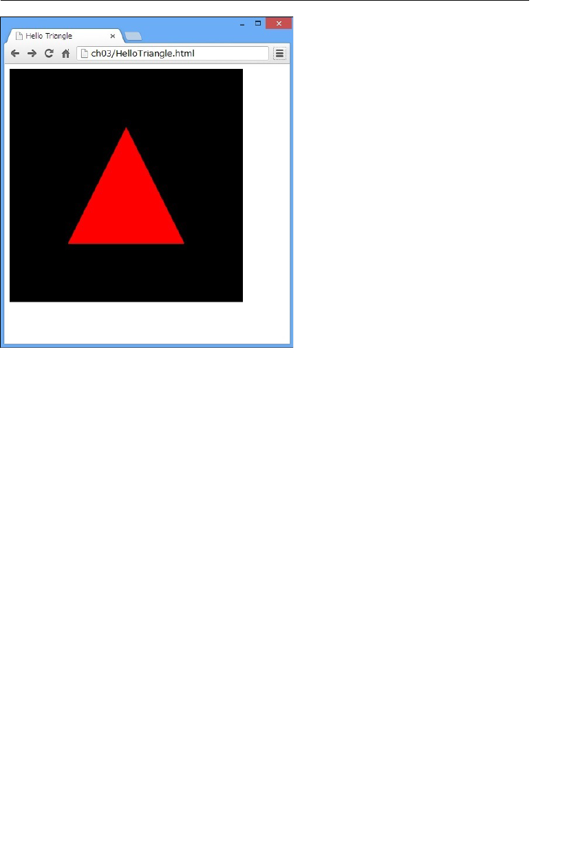
ptg11539634

WebGL Programming Guide

xxii

Figure P.1 Loading HelloTriangle results in a red triangle

If you don’t see the red triangle shown in the figure, take a look at Appendix H , which

explains how to change your browser settings to load WebGL.

Sample Programs and Related Links

All sample programs in this book and related links are available on the compan-

ion websites. The official site hosted by the publisher is www.informit.com/

title/9780321902924 and the author site is hosted at https://sites.google.com/site/

webglbook/ .

The latter site contains the links to each sample program in this book. You can run each

one directly by clicking the links.

If you want to modify the sample programs, you can download the zip file of all the

samples, available on both sites, to your local disk. In this case, you should note that

the sample program consists of both the HTML file and the associated JavaScript file

in the same folder. For example, for the sample program

HelloTriangle , you need

both

HelloTriangle.html and HelloTriangle.js . To run HelloTriangle , double-click

HelloTriangle.html .

ptg11539634

xxiii

Preface

Style Conventions

These style conventions are used in this book:

• Bold —First occurrences of key terms and important words

• Italic —Parameter names and names of references

• Monospace —Code examples, methods, functions, variables, command options,

JavaScript object names,  lenames, and HTML tags

ptg11539634

WebGL Programming Guide

xxiv

Acknowledgments

We have been fortunate to receive help and guidance from many talented individuals

during the process of creating this book, both with the initial Japanese version and the

subsequent English one.

Takafumi Kanda helped by providing numerous code samples for our support librar-

ies and sample programs; without him, this book could not have been realized. Yasuko

Kikuchi, Chie Onuma, and Yuichi Nishizawa provided valuable feedback on early versions

of the book. Of particular note, one insightful comment by Ms. Kikuchi literally stopped

the writing, causing a reevaluation of several sections and leading to a much stronger

book. Hiroyuki Tanaka and Kazsuhira Oonishi (iLinx) gave excellent support with the

sample programs, and Teruhisa Kamachi and Tetsuo Yoshitani supported the writing of

sections on HTML5 and JavaScript. The WebGL working group, especially Ken Russell

(Google), Chris Marin (Apple), and Dan Ginsburg (AMD), have answered many techni-

cal questions. We have been privileged to receive an endorsement from the president

of the Khronos Group, Neil Trevett, and appreciate the help of Hitoshi Kasai (Principal,

MIACIS Associates) who provided the connection to Mr. Trevett and the WebGL working

group. In addition, thank you to Xavier Michel and Makoto Sato (Sophia University), who

greatly helped with the translation of the original text and issues that arose during the

translation. For the English version, Jeff Gilbert, Rick Rafey, and Daniel Haehn reviewed

this book carefully and gave us excellent technical comments and feedback that greatly

improved the book. Our thanks also to Laura Lewin and Olivia Basegio from Pearson, who

have helped with organizing the publication and ensuring the whole process has been as

smooth and as painless as possible.

We both owe a debt of gratitude to the authors of the “Red Book” (OpenGL Programming

Guide) and the “Gold Book” (OpenGL ES 2.0 Programming Guide) both published by

Pearson, without which this book would not have been possible. We hope, in some small

way, that this book repays some of that debt.

ptg11539634

xxv

About the Authors

Dr. Kouichi Matsuda has a broad background in user interface and user experience design

and its application to novel multimedia products. His work has taken him from product

development, through research, and back to development, having spent time at NEC,

Sony Corporate Research, and Sony Computer Science Laboratories. He is currently a chief

distinguished researcher focused on user experience and human computer interaction

across a range of consumer electronics. He was the designer of the social 3D virtual world

called “PAW” (personal agent-oriented virtual world), was involved in the development

of the VRML97 (ISO/IEC 14772-1:1997) standard from the start, and has remained active

in both VRML and X3D communities (precursors to WebGL). He has written 15 books on

computer technologies and translated a further 25 into Japanese. His expertise covers user

experiences, user interface, human computer interaction, natural language understanding,

entertainment-oriented network services, and interface agent systems. Always on

the lookout for new and exciting possibilities in the technology space, he combines his

professional life with a love of hot springs, sea in summer, wines, and MANGA (at

which he dabbles in drawing and illustrations). He received his Ph.D. (Engineering)

from the Graduate School of Engineering, University of Tokyo, and can be reached via

WebGL.prog.guide@gmail.com .

Dr. Rodger Lea is an adjunct professor with the Media and Graphics Interdisciplinary

Centre at the University of British Columbia, with an interest in systems aspects of multi-

media and distributed computing. With more than 20 years of experience leading research

groups in both academic and industrial settings, he has worked on early versions of shared

3D worlds, helped define VRML97, developed multimedia operating systems, prototyped

interactive digital TV, and led developments on multimedia home networking standards.

He has published more than 60 research papers and three books, and he holds 12 patents.

His current research explores the growing “Internet of Things,” but he retains a passion

for all things media and graphics.

ptg11539634

This page intentionally left blank

ptg11539634

Chapter 1

Overview of WebGL

WebGL is a technology that enables drawing, displaying, and interacting with sophisticated

interactive three-dimensional computer graphics (“3D graphics”) from within web browsers.

Traditionally, 3D graphics has been restricted to high-end computers or dedicated game consoles

and has required complex programming. However, as both personal computers and, more impor-

tantly, web browsers, have become more sophisticated, it has become possible to create and

display 3D graphics using accessible and well-known web technologies. WebGL, when combined

with HTML5 and JavaScript, makes 3D graphics accessible to web developers and will play an

important role in the development of next generation, easy-to-use and intuitive user interfaces

and web content. Some examples of this are shown in Figure 1.1 . Over the next few years, you

can expect to see WebGL used on a range of devices from standard PCs to consumer electronics,

smart phones, and tablets.

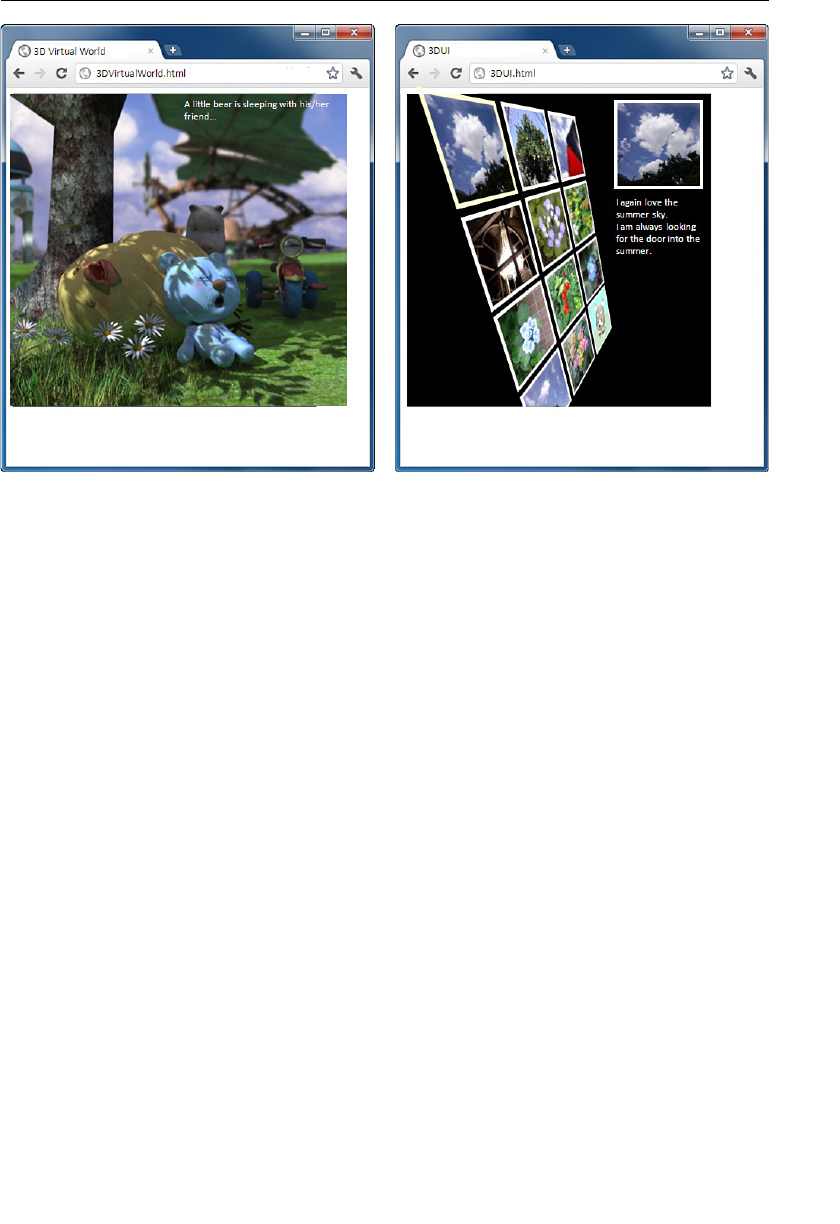
ptg11539634

CHAPTER 1 Overview of WebGL

Kouichi Matsuda (right)

HTML5, the latest evolution of the HTML standard, expands traditional HTML with

features covering 2D graphics, networking, and local storage access. With the advent of

HTML5, browsers are rapidly evolving from simple presentation engines to sophisticated

application platforms. With this evolution comes a need for interface and graphics capa-

bilities beyond 2D. WebGL has been designed for that central role of creating the visual

layer for new browser-based 3D applications and experiences.

Traditionally, creating compelling 3D graphics required you to create a stand-alone appli-

cation using a programming language such as C or C++ along with dedicated computer

graphics libraries such as OpenGL and Direct3D. However, with WebGL, you can now

realize 3D graphics as part of a standard web page using familiar HTML and JavaScript—

with a little extra code for the 3D graphics.

Importantly, because WebGL is supported as the browser’s default built-in technology for

rendering 3D graphics, you can use WebGL directly without having to install special plug-

ins or libraries. Better still, because it’s all browser based, you can run the same WebGL

applications on various platforms, from sophisticated PCs down to consumer electronics,

tablets, and smart phones.

This chapter briefly introduces you to WebGL, outlines some of the key features and

advantages of WebGL, and discusses its origins. It also explains the relationship of WebGL

to HTML5 and JavaScript and the structure of WebGL programs.

ptg11539634

Advantages of WebGL 3

Advantages of WebGL

As HTML has evolved, web developers have been able to create increasingly sophisticated

web-based applications. Originally, HTML offered only static content, but the introduc-

tion of scripting support like JavaScript enabled more complex interactions and dynamic

content. HTML5 introduced further sophistication, including support for 2D graphics via

the canvas tag. This allowed a variety of graphical elements on a web page, ranging from

dancing cartoon characters to map animations that respond to user input by updating the

maps in real time.

WebGL takes this one step further, enabling the display and manipulation of 3D graphics

on web pages by using JavaScript. Using WebGL, it becomes possible to create rich user

interfaces and 3D games and to use 3D to visualize and manipulate a variety of informa-

tion from the Internet. Although the technical capabilities of WebGL are impressive, it is

perhaps the ease of use and accessibility that differentiate it from other technologies and

that will ensure its impact. In particular:

• You can start developing 3D graphics applications using only a text editor and

browser.

• You can easily publish the 3D graphics applications using standard web technolo-

gies, making them available to your friends or other web users.

• You can leverage the full functionality of the browser.

• Learning and using WebGL is easy because a lot of material is already available for

study and development.

You Can Start Developing 3D Graphics Applications Using Only

a Text Editor

One handy and convenient point in developing applications using WebGL is that you

don’t need to set up an application developing environment for WebGL. As explained

earlier, because WebGL is built into the browser, there is no need for special applica-

tion development tools such as compilers and linkers to create 3D graphics applications.

As a minimum, to view the sample programs explained in this book, you only need a

WebGL-enabled browser. If you want to edit them or create your own, a standard text

editor (for example, Notepad or TextEdit) is enough. In Figure 1.2 , you can see a WebGL

application running in Chrome and the HTML file opened in Notepad. The JavaScript file

(

RotateObject.js ) that uses WebGL is loaded by the HTML file and could also be edited

using a simple text editor.

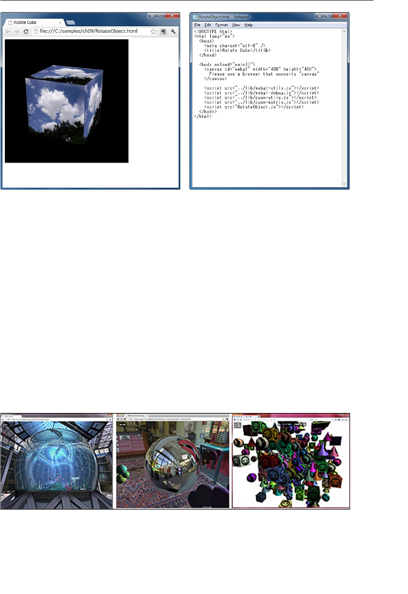
ptg11539634

CHAPTER 1 Overview of WebGL

Browser (Chrome) Notepad

Figure 1.2 The only tools needed for developing 3D graphics applications using WebGL

Publishing Your 3D Graphics Applications Is Easy

Traditionally, 3D graphics applications have been developed using a programming

language such as C or C++ and then compiled into an executable binary for a specific plat-

form. This meant, for example, the version for a Macintosh wouldn’t work on Windows or

Linux. Additionally, users often needed to install not only the applications themselves but

also libraries required by the applications to run, which meant another level of complexity

when you wanted to share your work.

In contrast, because WebGL applications are composed of HTML and JavaScript files,

they can be easily shared by simply putting them on a web server just like standard web

pages or distributing the HTML and JavaScript files via email. For example, Figure 1.3

shows some sample WebGL applications published by Google and available at http://code.

google.com/p/webglsamples/ .

Figure 1.3 WebGL sample applications published by Google (with the permission of Gregg

Tavares, Google)

ptg11539634

Origins of WebGL 5

You Can Leverage the Full Functionality of the Browser

Because WebGL applications are created as part of a web page, you can utilize the full

functionality of the browser such as arranging buttons, displaying dialog boxes, drawing

text, playing video or audio, and communicating with web servers. These advanced

features come for free, whereas in traditional 3D graphics applications they would need to

be programmed explicitly.

Learning and Using WebGL Is Easy

The specification of WebGL is based on the royalty-free open standard, OpenGL, which

has been widely used in graphics, video games, and CAD applications for many years. In

one sense, WebGL is “OpenGL for web browsers.” Because OpenGL has been used in a

variety of platforms over the past 20 years, there are many reference books, materials, and

sample programs using OpenGL, which can be used to better understand WebGL.

Origins of WebGL

Two of the most widely used technologies for displaying 3D graphics on personal comput-

ers are Direct3D and OpenGL. Direct3D, which is part of Microsoft’s DirectX technologies,

is the 3D graphics technology primarily used on Windows platforms and is a proprietary

application programming interface (API) that Microsoft controls. An alternative, OpenGL

has been widely used on various platforms due to its open and royalty-free nature.

OpenGL is available for Macintosh, Linux, and a variety of devices such as smart phones,

tablet computers, and game consoles (PlayStation and Nintendo). It is also well supported

on Windows and provides an alternative to Direct3D.

OpenGL was originally developed by Silicon Graphics Inc. and published as an open

standard in 1992. OpenGL has evolved through several versions since 1992 and has had a

profound effect on the development of 3D graphics, software product development, and

even film production over the years. The latest version of OpenGL at the time of writing

is version 4.3 for desktop PCs. Although WebGL has its roots in OpenGL, it is actually

derived from a version of OpenGL designed specifically for embedded computers such as

smart phones and video game consoles. This version, known as OpenGL ES (for Embedded

Systems), was originally developed in 2003–2004 and was updated in 2007 (ES 2.0) and

again in 2012 (ES 3.0). WebGL is based on the ES 2.0 version. In recent years, the number

of devices and processors that support the specification has rapidly increased and includes

smart phones (iPhone and Android), tablet computers, and game consoles. Part of the

reason for this successful adoption has been that OpenGL ES added new features but also

removed many unnecessary or old-fashioned features from OpenGL, resulting in a light-

weight specification that still had enough visual expressive power to realize attractive 3D

graphics.

Figure 1.4 shows the relationship among OpenGL, OpenGL ES 1.1/2.0/3.0, and WebGL.

Because OpenGL itself has continued to evolve from 1.5, to 2.0, to 4.3, OpenGL ES

have been standardized as a subset of specific versions of OpenGL (OpenGL 1.5 and

OpenGL 2.0).

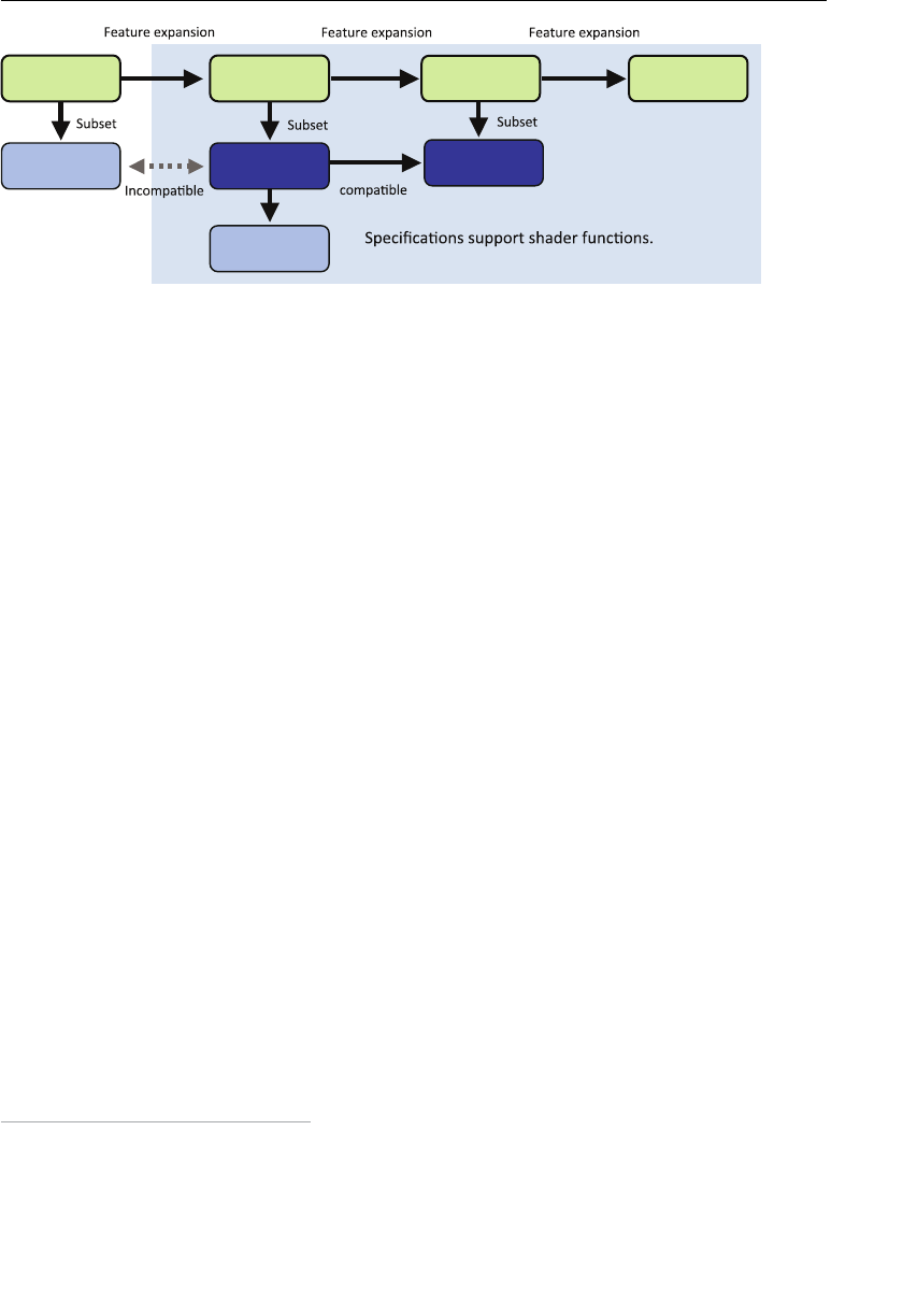
ptg11539634

CHAPTER 1 Overview of WebGL

5 . 1 L G n e p O 0 . 2 L G n e p O

S E L G n e p O

1 . 1

S E L G n e p O

0 . 2

3 . 3 L G n e p O

0 . 1 L G b e W

S E L G n e p O

0 . 3

3 . 4 L G n e p O

Figure 1.4 Relationship among OpenGL, OpenGL ES 1.1/2.0/3.0, and WebGL

As shown in Figure 1.4 , with the move to OpenGL 2.0, a significant new capability,

programmable shader functions , was introduced. This capability has been carried

through to OpenGL ES 2.0 and is a core part of the WebGL 1.0 specification.

Shader functions or shaders are computer programs that make it possible to program

sophisticated visual effects by using a special programming language similar to C. This

book explains shader functions in a step-by-step manner, allowing you to quickly master

the power of WebGL. The programming language that is used to create shaders is called

a shading language . The shading language used in OpenGL ES 2.0 is based on the

OpenGL shading language (GLSL) and referred to as OpenGL ES shading language

(GLSL ES). Because WebGL is based on OpenGL ES 2.0, it also uses GLSL ES for creating

shaders.

The Khronos Group (a non-profit industry consortium created to develop, publish, and

promote various open standards) is responsible for the evolution and standardization of

OpenGL. In 2009, Khronos established the WebGL working group and then started the

standardization process of WebGL based on OpenGL ES 2.0, releasing the first version of

WebGL in 2011. This book is written based primarily on that specification and, where

needed, the latest specification of WebGL published as an Editor’s Draft. For more infor-

mation, please refer to the specification.

Structure of WebGL Applications

In HTML, dynamic web pages can be created by using a combination of HTML and

JavaScript. With the introduction of WebGL, the shader language GLSL ES needs to

be added to the mix, meaning that web pages using WebGL are created by using three

1 WebGL 1.0: www.khronos.org/registry/webgl/specs/1.0/ and Editor’s draft: www.khronos.org/

registry/webgl/specs/latest/

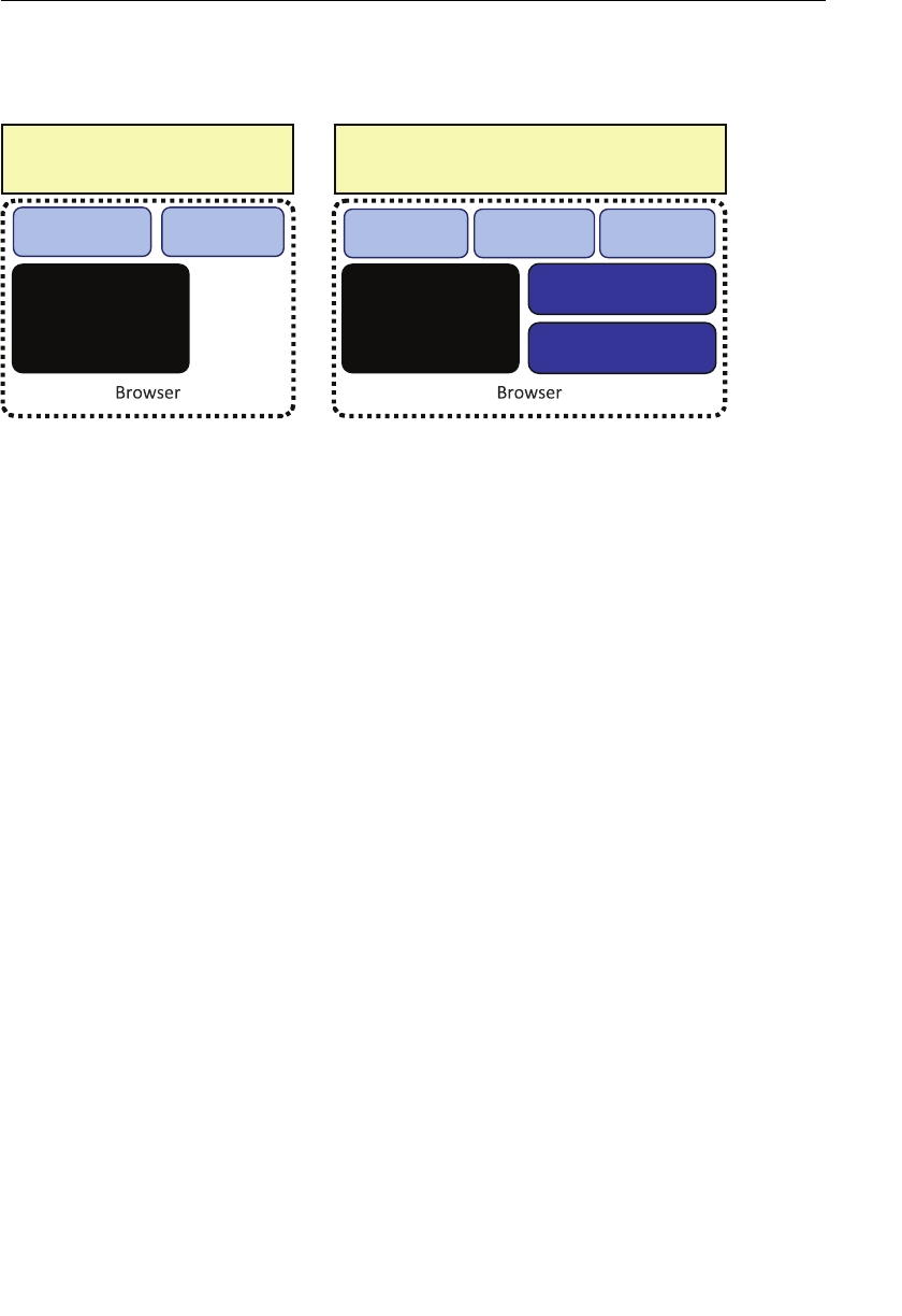
ptg11539634

Summary 7

languages: HTML5 (as a Hypertext Markup Language), JavaScript, and GLSL ES. Figure 1.5

shows the software architecture of traditional dynamic web pages (left side) and web pages

using WebGL (right side).

5 L M T H t p i r c S a v a J S E L S L G

L G b e W g n i s u e g a p b e W

L M T H t p i r c S a v a J

e g a p b e W

L M T H L G b e W

S E L G n e p O / L G n e p O

enignEgniredneR

HTML

LMTH

enignEgniredneR

Figure 1.5 The software architecture of dynamic web pages (left) and web pages using

WebGL (right)

However, because GLSL ES is generally written within JavaScript, only HTML and

JavaScript files are actually necessary for WebGL applications. So, although WebGL does

add complexity to the JavaScript, it retains the same structure as standard dynamic web

pages, only using HTML and JavaScript files.

Summary

This chapter briefly overviewed WebGL, explained some key features, and outlined

the software architecture of WebGL applications. In summary, the key takeaway from

this chapter is that WebGL applications are developed using three languages: HTML5,

JavaScript, and GLSL ES—however, because the shader code (GLSL ES) is generally embed-

ded in the JavaScript, you have exactly the same file structure as a traditional web page.

The next chapter explains how to create applications using WebGL, taking you step by

step through a set of simple WebGL examples.

ptg11539634

This page intentionally left blank

ptg11539634

Chapter 2

Your First Step with WebGL

As explained in Chapter 1 , “Overview of WebGL,” WebGL applications use both HTML and

JavaScript to create and draw 3D graphics on the screen. To do this, WebGL utilizes the new

<canvas> element, introduced in HTML5, which defines a drawing area on a web page. Without

WebGL, the

<canvas> element only allows you to draw two-dimensional graphics using

JavaScript. With WebGL, you can use the same element for drawing three-dimensional graphics.

This chapter explains the

<canvas> element and the core functions of WebGL by taking you,

step-by-step, through the construction of several example programs. Each example is written in

JavaScript and uses WebGL to display and interact with a simple shape on a web page. Because of

this, these JavaScript programs are referred to as WebGL applications .

The example WebGL applications will highlight some key points, including:

• How WebGL uses the <canvas> element and how to draw on it

• The linkage between HTML and WebGL using JavaScript

• Simple WebGL drawing functions

• The role of shader programs within WebGL

By the end of this chapter, you will understand how to write and execute basic WebGL applica-

tions and how to draw simple 2D shapes. You will use this knowledge to explore further the

basics of WebGL in Chapters 3 , “Drawing and Transforming Triangles,” 4 , “More Transformations

and Basic Animation,” and 5 , “Using Colors and Texture Images.”

What Is a Canvas?

Before HTML5, if you wanted to display an image in a web page, the only native HTML approach

was to use the

<img> tag. This tag, although a convenient tool, is restricted to still images and

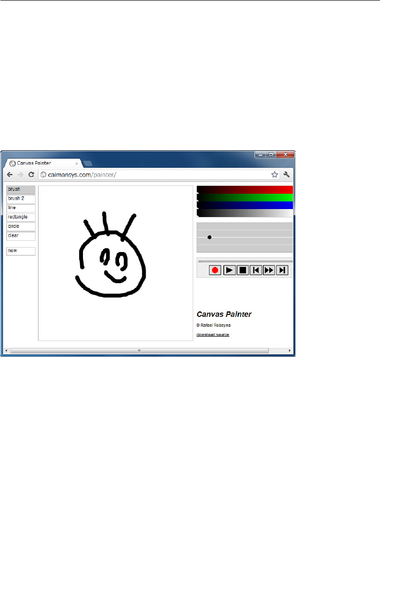
ptg11539634

CHAPTER 2 Your First Step with WebGL

doesn’t allow you to dynamically draw and display the image on the fly. This is one of the

reasons that non-native solutions such as Flash Player have been used.

However, HTML5, by introducing the

<canvas> tag, has changed all that, offering a conve-

nient way to draw computer graphics dynamically using JavaScript.

In a similar manner to the way artists use paint canvases, the

<canvas> tag defines a

drawing area on a web page. Then, rather than using brush and paints, you can use

JavaScript to draw anything you want in the area. You can draw points, lines, rectangles,

circles, and so on by using JavaScript methods provided for

<canvas> . Figure 2.1 shows an

example of a drawing tool that uses the

<canvas> tag.

Figure 2.1 A drawing tool using the <canvas> element ( http://caimansys.com/painter/ )

This drawing tool runs within a web page and allows you to interactively draw lines, rect-

angles, and circles and even change their colors.

Although you won’t be creating anything as sophisticated just yet, let’s look at the core

functions of

<canvas> by using a sample program, DrawRectangle , which draws a filled

blue rectangle on a web page. Figure 2.2 shows

DrawRectangle when it’s loaded into a

browser.

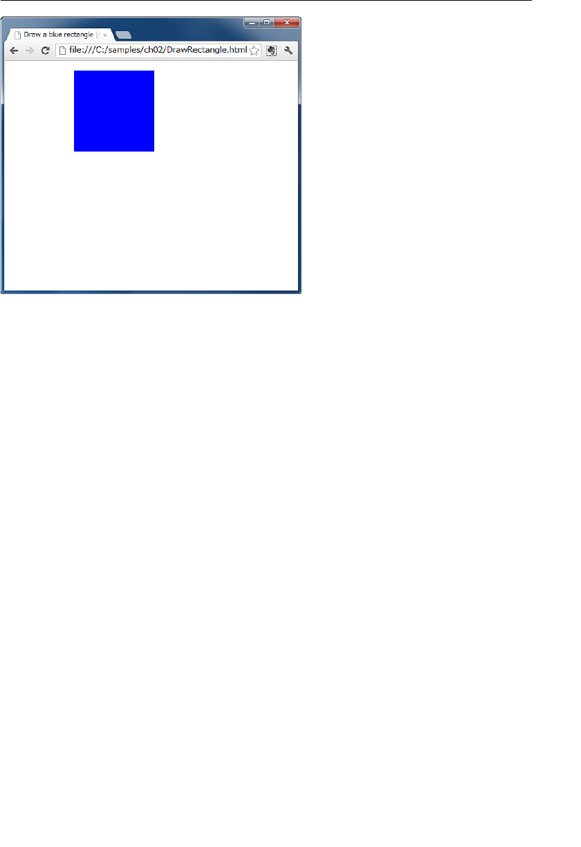
ptg11539634

What Is a Canvas? 11

Figure 2.2 DrawRectangle

Using the <canvas> Tag

Let’s look at how DrawRectangle works and explain how the <canvas> tag is used in the

HTML file. Listing 2.1 shows

DrawingTriangle.html . Note that all HTML files in this book

are written in HTML5.

Listing 2.1 DrawRectangle.html

1 <!DOCTYPE html>

2 <html lang=»en»>

3 <head>

4 <meta charset=»utf-8″ />

5 <title>Draw a blue rectangle (canvas version)</title>

6 </head>

8 <body onload=»main()»>

9 <canvas id=»example» width=»400″ height=»400″>

10 Please use a browser that supports «canvas»

11 </canvas>

12 <script src=»DrawRectangle.js»></script>

13 </body>

14 </html>

ptg11539634

CHAPTER 2 Your First Step with WebGL

The <canvas> tag is defined at line 9. This defines the drawing area as a 400 × 400 pixel

region on a web page using the

width and height attributes in the tag. The canvas is given

an identifier using the

id attribute, which will be used later:

By default, the canvas is invisible (actually transparent) until you draw something into it,

which we’ll do with JavaScript in a moment. That’s all you need to do in the HTML file to

prepare a

<canvas> that the WebGL program can use. However, one thing to note is that

this line only works in a

<canvas> -enabled browser. However, browsers that don’t support

the

<canvas> tag will ignore this line, and nothing will be displayed on the screen. To

handle this, you can display an error message by adding the message into the tag as

follows:

9 <canvas id=»example» width=»400″ height=»400″>

10 Please use a browser that supports «canvas»

11 </canvas>

To draw into the canvas, you need some associated JavaScript code that performs the

drawing operations. You can include that JavaScript code in the HTML or write it as a

separate JavaScript file. In our examples, we use the second approach because it makes the

code easier to read. Whichever approach you take, you need to tell the browser where the

JavaScript code starts. Line 8 does that by telling the browser that when it loads the sepa-

rate JavaScript code it should use the function

main() as the entry point for the JavaScript

program. This is specified for the

<body> element using its onload attribute that tells the

browser to execute the JavaScript function

main() after it loads the <body> element:

8 <body onload=»main()»>

Line 12 tells the browser to import the JavaScript file DrawRectangle.js in which the

function

main() is defined:

12 <script src=»DrawRectangle.js»></script>

For clarity, all sample programs in this book use the same filename for both the HTML file

and the associated JavaScript file, which is imported in the HTML file (see Figure 2.3 ).

ptg11539634

What Is a Canvas? 13

>lmth EPYTCOD!<

>«ne“=gnal lmth<

>daeh<

>/ «8—ftu«=tesrahc atem<

>eltit/<)noisrev savnac( elgnatcer eulb a warD>eltit<

>daeh/<

>«)(niam«=daolno ydob<

>«051«=thgieh «002«=htdiw «elpmaxe«=di savnac

”savnac“ stroppus taht resworb a esu esaelP

>savnac/<

>tpircs/<>«sj.elgnatceRwarD«=crs tpircs<

>ydob/<

>lmth/<

sj.elgnatceRwarD //

{ )(niam noitcnuf

tnemele >savnac< eht eveirteR //

;)‘elpmaxe‘(dIyBtnemelEteg.tnem

ucod = savnac rav

{ )savnac!( fi

;)‘ tnemele >savnac< eht eveirter ot deliaF(gol.elosnoc

;eslaf

nruter

}

GCD2 rof txetnoc gniredner eht teG //

;)‘d

2‘(txetnoCteg.savnac = xtc rav

elgnatcer eul

b a warD //

roloc eulb a teS // ;‘)0.1 ,552

,0 ,0(abgr‘ = elytSllif.xtc

roloc eht htiw elgnatcer a

lliF

// ;)051 ,051 ,01 ,021(tceRllif.xtc

}

lmth.elgnatceRwarD

sj.elgnatceRwarD

Figure 2.3 DrawRectangle.html and DrawRectangle.js

DrawRectangle.js

DrawRectangle.js is a JavaScript program that draws a blue rectangle on the drawing area

defined by the

<canvas> element (see Listing 2.2 ). It has only 16 lines, which consist of

the three steps required to draw two-dimensional computer graphics (2D graphics) on the

canvas:

1. Retrieve the

<canvas> element.

2. Request the rendering “context” for the 2D graphics from the element.

3. Draw the 2D graphics using the methods that the context supports.

These three steps are the same whether you are drawing a 2D or a 3D graphic; here, you

are drawing a simple 2D rectangle using standard JavaScript. If you were drawing a 3D

graphic using WebGL, then the rendering context in step (2) at line 11 would be for a 3D

rendering context; however, the high-level process would be the same.

Listing 2.2 DrawRectangle.js

1 // DrawRectangle.js

2 function main() {

3 // Retrieve <canvas> element <- (1)

4 var canvas = document.getElementById(‘example’);

5 if (!canvas) {

6 console.log(‘Failed to retrieve the <canvas> element’);

7 return;

8 }

10 // Get the rendering context for 2DCG <- (2)

11 var ctx = canvas.getContext(‘2d’);

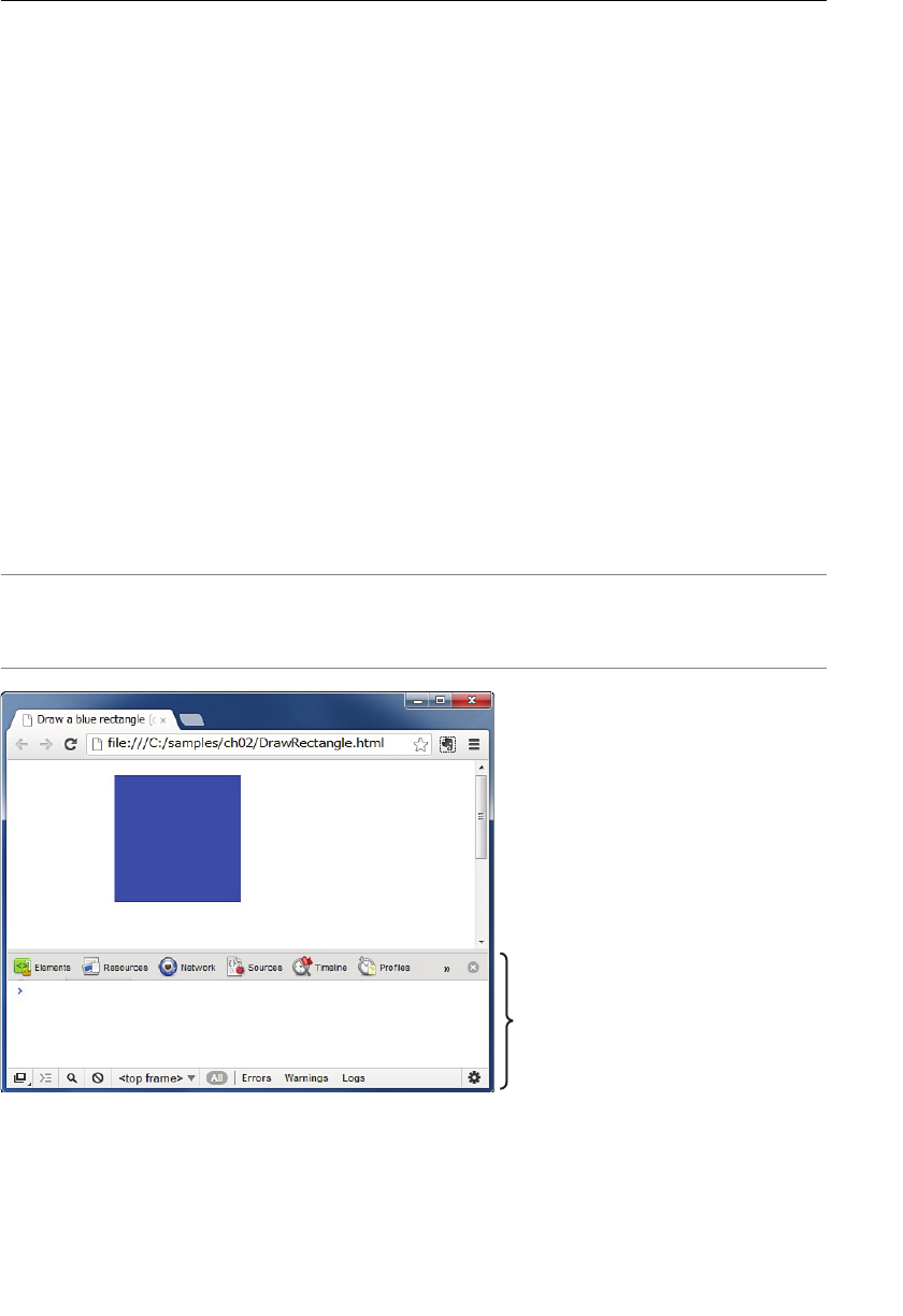
ptg11539634

CHAPTER 2 Your First Step with WebGL

13 // Draw a blue rectangle <- (3)

14 ctx.fillStyle = ‘rgba(0, 0, 255, 1.0)’; // Set a blue color

15 ctx.fillRect(120, 10, 150, 150); // Fill a rectangle with the color

16 }

Let us look at each step in order.

Retrieve the <canvas> Element

To draw something on a

<canvas> , you must first retrieve the <canvas> element from the

HTML file in the JavaScript program. You can get the element by using the method

docu-

ment.getElementById() , as shown at line 4. This method has a single parameter, which is

the string specified in the attribute

id in the <canvas> tag in our HTML file. In this case,

the string is

‘example’ and it was defined back in DrawRectangle.html at line 9 (refer to

Listing 2.1 ).

If the return value of this method is not

null , you have successfully retrieved the element.

However, if it is

null , you have failed to retrieve the element. You can check for this

condition using a simple

if statement like that shown at line 5. In case of error, line 6 is

executed. It uses the method

console.log() to display the parameter as a string in the

browser’s console.

Note In Chrome, you can show the console by going to Tools, JavaScript Console or

pressing Ctrl+Shift+J (see Figure 2.4 ); in Firefox, you can show it by going to Tools, Web

Developer, Web Console or pressing Ctrl+Shift+K.

Console

Figure 2.4 Console in Chrome

ptg11539634

What Is a Canvas? 15

Get the Rendering Context for the 2D Graphics by Using the Element

Because the

<canvas> is designed to be flexible and supports both 2D and 3D, it does not

provide drawing methods directly and instead provides a mechanism called a context ,

which supports the actual drawing features. Line 11 gets that context:

11 var ctx = canvas.getContext(‘2d’);

The method canvas.getContext() has a parameter that specifies which type of drawing

features you want to use. In this example you want to draw a 2D shape, so you must

specify 2d (case sensitive).

The result of this call, the context, is stored in the variable

ctx ready for use. Note, for

brevity we haven’t checked error conditions, which is something you should always do in

your own programs.

Draw the 2D Graphics Using the Methods Supported by the Context

Now that we have a drawing context, let’s look at the code for drawing a blue rectangle,

which is a two-step process. First, set the color to be used when drawing. Second, draw (or

fill) a rectangle with the color.

Lines 14 and 15 handle these steps:

13 // Draw a blue rectangle <- (3)

14 ctx.fillStyle = ‘rgba(0, 0, 255, 1.0)’; // Set color to blue

15 ctx.fillRect(120, 10, 150, 150); // Fill a rectangle with the color

The rgba in the string rgba(0, 0, 255, 1.0) on line 14 indicate r (red), g (green), b

(blue), and a (alpha: transparency), with each RGB parameter taking a value from 0

(minimum value) to 255 (maximum value) and the alpha parameter from 0.0 (transpar-

ent) to 1.0 (opaque). In general, computer systems represent a color by using a combina-

tion of red, green, and blue (light’s three primary colors), which is referred to as RGB

format . When alpha (transparency) is added, the format is called RGBA format .

Line 15 then uses the

fillStyle property to specify the fill color when drawing the rect-

angle. However, before going into the details of the arguments on line 15, let’s look at the

coordinate system used by the

<canvas> element (see Figure 2.5 ).

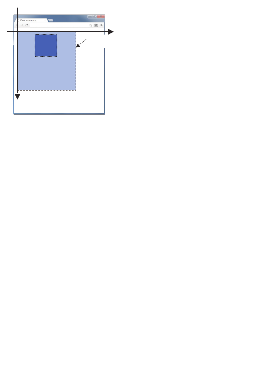
ptg11539634

CHAPTER 2 Your First Step with WebGL

>savnac<

aera gniward

)0 ,0(

)004 ,004(

)01 ,021(

Figure 2.5 The coordinate system of <canvas>

As you can see in the figure, the coordinate system of the

<canvas> element has the hori-

zontal direction as the x-axis (right-direction is positive) and the vertical direction as the

y-axis (down-direction is positive). Note that the origin is located at the upper-left corner

and the down direction of the y-axis is positive. The rectangle drawn with a dashed line

is the original

<canvas> element in our HTML file (refer to Listing 2.1 ), which we speci-

fied as being 400 by 400 pixels. The dotted line is the rectangle that the sample program

draws.

When we use

ctx.fillRect() to draw a rectangle, the first and second parameters of this

method are the position of the upper-left corner of the rectangle within the

<canvas> , and

the third and fourth parameters are the width and height of the rectangle (in pixels):

15 ctx.fillRects(120, 10, 150, 150);// Fill a rectangle with the color

After loading DrawRectangle.html into your browser, you will see the rectangle that was

shown in Figure 2.2 .

So far, we’ve only looked at 2D graphics. However, WebGL also utilizes the same

element to draw 3D graphics on a web page, so let’s now enter into the WebGL world.

The World’s Shortest WebGL Program:

Clear Drawing Area

Let’s start by constructing the world’s shortest WebGL program, HelloCanvas , which

simply clears the drawing area specified by a

<canvas> tag. Figure 2.6 shows the result of

loading the program, which clears (by filling with black) the rectangular area defined by a

<canvas> .

ptg11539634

The World’s Shortest WebGL Program: Clear Drawing Area 17

Figure 2.6 HelloCanvas

The HTML File (HelloCanvas.html)

Take a look at HelloCanvas.html , as shown in Figure 2.7 ). Its structure is simple and starts

by defining the drawing area using the

<canvas> element at line 9 and then importing

HelloCanvas.js (the WebGL program) at line 16.

Lines 13 to 15 import several other JavaScript files, which provide useful convenience

functions that help WebGL programming. These will be explained in more detail later. For

now, just think of them as libraries.

ptg11539634

CHAPTER 2 Your First Step with WebGL

>lmthEPYTCOD!<1

>”ne”=gnallmth<2

>daeh<3

>/«8—ftu«=tesrahcatem<4

>eltit/<savnacraelC>eltit<5

>daeh/<6

>«)(

niam«=daolnoydob<8

>«004«=thgieh«004«=htdiw«lgbew«=disavnac<9

«savnac«gnitroppusresworbehtesuesaelP01

>savnac/<11

>tpircs/<>«sj.slitu—lgbew/bil/..«=crstpircs<31

>tpircs/<>«sj.gubed—lgbew/bil/..«=crstpircs<

>tpircs/<>«sj.slitu—nouc/bil/..«=crstpircs<51

>tpircs/<>«sj.savnaColleH«=crstpircs<61

>ydob/<71

>lmth/<81

hcihwotni>savnac<

sepahsswardLGbeW

seliftpircSavaJ

tneinevnocgniniatnoc

LGbeWrofsnoitcnuf

gniwardeliftpirc

SavaJ

>savnac<ehtotnisepahs

Figure 2.7 HelloCanvas.html

You’ve set up the canvas (line 9) and then imported the

HelloCanvas JavaScript file (line

16), which actually uses WebGL commands to access the canvas and draw your first 3D

program. Let us look at the WebGL program defined in

HelloCanvas.js .

JavaScript Program (HelloCanvas.js)

HelloCanvas.js (see Listing 2.3 ) has only 18 lines, including comments and error

handling, and follows the same steps as explained for 2D graphics: retrieve the

element, get its rendering context, and then begin drawing.

Listing 2.3 HelloCanvas.js

1 // HelloCanvas.js

2 function main() {

3 // Retrieve <canvas> element

4 var canvas = document.getElementById(‘webgl’);

6 // Get the rendering context for WebGL

7 var gl = getWebGLContext(canvas);

8 if (!gl) {

9 console.log(‘Failed to get the rendering context for WebGL’);

10 return;

11 }

ptg11539634

The World’s Shortest WebGL Program: Clear Drawing Area 19

13 // Specify the color for clearing <canvas>

14 gl.clearColor(0.0, 0.0, 0.0, 1.0);

16 // Clear <canvas>

17 gl.clear(gl.COLOR_BUFFER_BIT);

18 }

As in the previous example, there is only one function, main() , which is the link between

the HTML and the JavaScript and set at

<body> element using its onload attribute (line

HelloCanvas.html (refer to Figure 2.7 ).

Figure 2.8 shows the processing flow of the main() function of our WebGL program and

consists of four steps, which are discussed individually next.

L G b e W r o f t x e t n o c g n i r e d n e r e h t t e G

> s a v n a c < r a e l C

t n e m e l e > s a v n a c < e h t e v e i r t e R

> s a v n a c < g n i r a e l c r o l o c e h t t e S

Figure 2.8 The processing flow of the main() function

Retrieve the <canvas> Element

First,

main() retrieves the <canvas> element from the HTML file. As explained in

DrawRectangle.js , it uses the document.getElementById() method specifying webgl as the

argument. Looking back at

HelloCanvas.html (refer to Figure 2.7 ), you can see that attri-

bute

id is set at the <canvas> tag at line 9:

9 <canvas id=»webgl» width=»400″ height=»400″>

The return value of this method is stored in the canvas variable.

ptg11539634

CHAPTER 2 Your First Step with WebGL

Get the Rendering Context for WebGL

In the next step, the program uses the variable

canvas to get the rendering context

for WebGL. Normally, we would use

canvas.getContext() as described earlier to

get the rendering context for WebGL. However, because the argument specified in

canvas.getContext() varies between browsers,

1 we have written a special function

get WebGLContext() to hide the differences between the browsers:

7 var gl = getWebGLContext(canvas);

This is one of the convenience functions mentioned earlier that was written specially for

this book and is defined in

cuon-utils.js , which is imported at line 15 in HelloCanvas.

html . The functions defined in the file become available by specifying the path to the file

in the attribute

src in the <script> tag and loading the file. The following is the specifica-

tion of

getWebGLContext() .

getWebGLContext(element [, debug])

Get the rendering context for WebGL, set the debug setting for WebGL, and display any

error message in the browser console in case of error.

Parameters element Specifies

<canvas> element to be queried.

debug (optional) Default is

true . When set to true , JavaScript errors

are displayed in the console. Note: Turn off after

debugging; otherwise, performance is affected.

Return value non-null The rendering context for WebGL.

null WebGL is not available.

The processing flow to retrieve the

<canvas> element and use the element to get the

rendering context is the same as in

DrawRectangle.js shown earlier, where the rendering

context was used to draw 2D graphics on the

<canvas> .

In a similar way, WebGL uses the rendering context returned by getWebGLContext() to

draw on the

<canvas> . However, now the context is for 3D rather than 2D, so 3D (that is,

WebGL) methods are available. The program stores the context in the variable

gl at line

7. You can use any name for the variable. We have intentionally used

gl throughout this

book, because it aligns the names of the WebGL-related methods to that of OpenGL ES

2.0, which is the base specification of WebGL. For example,

gl.clearColor() at line 14

corresponds to

glClearColor() in OpenGL ES 2.0 or OpenGL:

14 gl.clearColor(0.0, 0.0, 0.0, 1.0);

1 Although most browsers are settling on “experimental-webgl” for this argument, not all do.

Additionally, over time, this will evolve to plain ‘webgl,’ so we have chosen to hide this.

ptg11539634

The World’s Shortest WebGL Program: Clear Drawing Area 21

This book explains all WebGL-related methods assuming that the rendering context is

held in the variable

gl .

Once you have the rendering context for WebGL, the next step is to use the context to set

the color for clearing the drawing area specified by the

<canvas> .

Set the Color for Clearing the <canvas>

In the previous section,

DrawRectangle.js set the drawing color before drawing the rect-

angle. In a similar way, with WebGL you need to set the color before actually clearing the

drawing area. Line 14 uses

gl.clearColor() to set the color in RGBA format.

gl.clearColor (red, green, blue, alpha)

Specify the clear color for a drawing area:

Parameters red Specifies the red value (from 0.0 to 1.0).

green Specifies the green value (from 0.0 to 1.0).

blue Specifies the blue value (from 0.0 to 1.0).

alpha Specifies an alpha (transparency) value (from 0.0 to 1.0).

0.0 means transparent and 1.0 means opaque.

If any of the values of these parameters is less than 0.0 or more than 1.0, it

is truncated into 0.0 or 1.0, respectively.

Return value None

Errors

2 None

The sample program calls

gl.clearColor (0.0, 0.0, 0.0, 1.0) at line 14, so black is specified

as the clear color. The followings are examples that specify other colors:

(1.0, 0.0, 0.0, 1.0) red

(0.0, 1.0, 0.0, 1.0) green

(0.0, 0.0, 1.0, 1.0) blue

(1.0, 1.0, 0.0, 1.0) yellow

(1.0, 0.0, 1.0, 1.0) purple

(0.0, 1.0, 1.0, 1.0) light blue

(1.0, 1.0, 1.0, 1.0) white

2 In this book, the item “errors” is shown for all speci cations of WebGL-related methods. This

indicates errors that cannot be represented by the return value of the method when the method will

result in as error. By default, the errors are not displayed, but they can be displayed in a JavaScript

console by specifying true as the second argument of getWebGLContext() .

ptg11539634

CHAPTER 2 Your First Step with WebGL

You might have noticed that in our 2D programming example in this chapter,

DrawRectangle , each value for color is specified from 0 to 255. However, because WebGL

is based on OpenGL, it uses the traditional OpenGL values from 0.0 to 1.0. The higher the

value is, the more intense the color becomes. Similarly, for the alpha parameter (fourth

parameter), the higher the value, the less transparent the color.

Once you specify the clear color, the color is retained in the WebGL system and not

changed until another color is specified by a call to

gl.clearColor() . This means you

don’t need to specify the clear color again if at some point in the future you want to clear

the area again using the same color.

Clear <canvas>

Finally, you can use

gl.clear() to clear the drawing area with the specified clear color:

17 gl.clear(gl.COLOR_BUFFER_BIT);

Note that the argument of this method is gl.COLOR_BUFFER_BIT , not, as you might expect,

the

<canvas> element that defines the drawing area to be cleared. This is because the

WebGL method

gl.clear() is actually relying on OpenGL, which uses a more sophisti-

cated model than simple canvases, instead using multiple underlying buffers. One such

buffer , the color buffer, is used in this example. By using

gl.COLOR_BUFFER_BIT , you are

telling WebGL to use the color buffer when clearing the canvas. WebGL uses a number of

buffers in addition to the color buffer, including a depth buffer and a stencil buffer. The

color buffer will be covered in detail later in this chapter, and you’ll see the depth buffer

in action in Chapter 7 , “Toward the 3D World.” The stencil buffer will not be covered in

this book because it is seldom used.

Clearing the color buffer will actually cause WebGL to clear the

<canvas> area on the web

page.

gl.clear(buffer)

Clear the specified buffer to preset values. In the case of a color buffer, the value (color)

specified by

gl.clearColor() is used.

Parameters buffer Specifies the buffer to be cleared. Bitwise

OR ( | ) operators are used

to specify multiple buffers.

gl.COLOR_BUFFER_BIT Specifies the color buffer.

gl.DEPTH_BUFFER_BIT Specifies the depth buffer.

gl.STENCIL_BUFFER_BIT Specifies the stencil buffer.

Return value None

Errors INVALID_VALUE buffer is none of the preceding three values.

ptg11539634

Draw a Point (Version 1) 23

If no color has been specified (that is, you haven’t made a call to gl.clearColor() ), then

the following default value is used (see Table 2.1 ).

Table 2.1 Default Values to Clear Each Buffer and Associated Methods

Buffer Name Default Value Setting Method

Color buffer (0.0, 0.0, 0.0, 0.0)

gl.clearColor(red, green, blue, alpha)

Depth buffer 1.0

gl.clearDepth(depth)

Stencil buffer 0 gl.clearStencil(s)

Now that you’ve read through and understand this simple WebGL example, you should

load

HelloCanvas into your browser to check that the drawing area is cleared to black.

Remember, you can run all the examples in the book directly from the companion

website. However, if you want to experiment with any, you need to download the exam-

ples from the book’s website to a location on your local disk. If you’ve done that, to load

the example, navigate to that location on your disk and load

HelloCanvas.html into your

browser.

Experimenting with the Sample Program

Let’s experiment a little with the sample program to become familiar with the way you

specify colors in WebGL by trying some other colors for the clear operation. Using your

favorite editor, rewrite Line 14 of

HelloCanvas.js as follows and save your modification

back to the original file:

14 gl.clearColor(0.0, 0.0, 1.0, 1.0);

After reloading HelloCanvas.html into your browser, HelloCanvas.js is also reloaded,

and then

main() is executed to clear the drawing area to blue. Try to use other colors and

check the result. For example,

gl.clearColor(0.5, 0.5, 0.5, 1.0) clears the area to

gray.

Draw a Point (Version 1)

In the previous section, you saw how to initialize WebGL and use some simple WebGL-

related methods. In this section, you are going to go one step further and construct a

sample program to draw the simplest shape of all: a point. The program will draw a red

point using 10 pixels at (0.0, 0.0, 0.0). Because WebGL deals with three-dimensional

graphics, three coordinates are necessary to specify the position of the point. You’ll be

introduced to coordinates later, but for now simply accept that a point drawn at (0.0, 0.0,

0.0) is displayed at the center of the

<canvas> area.

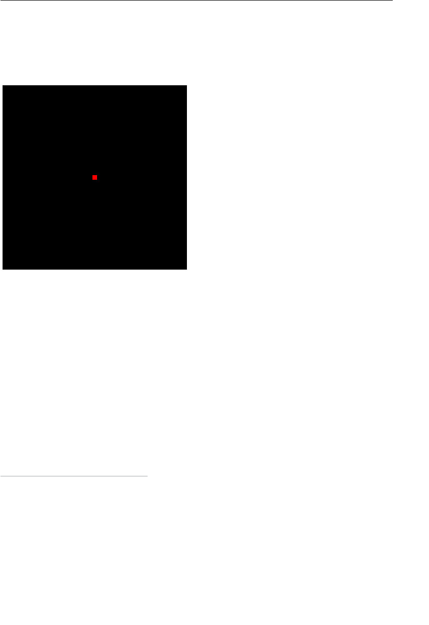
ptg11539634

CHAPTER 2 Your First Step with WebGL

The sample program name is HelloPoint1 and, as shown in Figure 2.9 , it draws a red

point (rectangle) at the center of the

<canvas> , which has been cleared to black.

3 You will

actually be using a filled rectangle as a point instead of a filled circle because a rectangle

can be drawn faster than a circle. (We will deal with how to draw a rounded point in

Chapter 9 , “Hierarchical Objects.”)

Figure 2.9 HelloPoint1

Just like clearing the color in the previous section, the color of a point must be specified

in RGBA. For red, the value of R is 1.0, G is 0.0, B is 0.0, and A is 1.0. You will remember

that

DrawRectangle.js earlier in the chapter specifies the drawing color and then draws a

rectangle as follows:

ctx.fillStyle=’rgba(0, 0, 255, 1.0)’;

ctx.fillRect(120, 10, 150, 150);

So you are probably thinking that WebGL would do something similar, perhaps some-

thing like this:

gl.drawColor(1.0, 0.0, 0.0, 1.0);

gl.drawPoint(0, 0, 0, 10); // The position of center and the size of point

The sample programs in Chapter 2 are written in the simplest way possible so the reader can focus

on understanding the functionality of shaders. In particular, they don’t use “buffer objects” (see

Chapter 3 ), which are generally used in WebGL. Although this helps by simplifying the explanation,

some browsers (especially Firefox) expect buffer objects and may fail to display correctly any

examples without them. In later chapters, and in actual application development, this will not

cause problems because you will be using “buffer objects.” However, if you are having problems, try

another browser. You can switch back in the next chapter.

ptg11539634

Draw a Point (Version 1) 25

Unfortunately, this is not possible. WebGL relies on a new type of drawing mechanism

called a shader , which offers a flexible and powerful mechanism for drawing 2D and 3D

objects and must be used by all WebGL applications. Shaders, although powerful, are

more complex, and you can’t just specify a simple draw command.

Because the shader is a critical core mechanism in WebGL programming that you will use

throughout this book, let’s examine it one step at a time so that you can understand it

easily.

HelloPoint1.html

Listing 2.4 shows HelloPoint1.html , which is functionally equivalent to HelloCanvas.

html (refer to Figure 2.7 ). The title of the web page and the JavaScript filename were

changed (lines 5 and 16), but everything else remains the same. From now on, unless

the HTML file is different from this example, we’ll skip showing the HTML files for the

examples.

Listing 2.4 HelloPoint1.html

1 <!DOCTYPE html>

2 <html lang=»en»>

3 <head>

4 <meta charset=»utf-8″ />

5 <title>Draw a point (1)</title>

6 </head>

8 <body onload=»main()»>

9 <canvas id=»webgl» width=»400″ height=»400″>

10 Please use the browser supporting «canvas».

11 </canvas>

13 <script src=»../libs/webgl-utils.js»></script>

14 <script src=»../libs/webgl-debug.js»></script>

15 <script src=»../libs/cuon-utils.js»></script>

16 <script src=»HelloPoint1.js»></script>

17 </body>

18 </html>

HelloPoint1.js

Listing 2.5 shows HelloPoint1.js . As you can see from the comments in the listing,

two “shader programs” are prepended to the JavaScript (lines 2 to 13). Glance through

the shader programs, and then go to the next section, where you’ll see more detailed

explanations.

ptg11539634

CHAPTER 2 Your First Step with WebGL

Listing 2.5 HelloPoint1.js

1 // HelloPoint1.js

2 // Vertex shader program

3 var VSHADER_SOURCE =

4 ‘void main() {n’ +

5 ‘ gl_Position = vec4(0.0, 0.0, 0.0, 1.0);n’ + // Coordinates

6 ‘ gl_PointSize = 10.0;n’ + // Set the point size

7 ‘}n’;

9 // Fragment shader program

10 var FSHADER_SOURCE =

11 ‘void main() {n’ +

12 ‘ gl_FragColor = vec4(1.0, 0.0, 0.0, 1.0);n’ + // Set the color

13 ‘}n’;

15 function main() {

16 // Retrieve <canvas> element

17 var canvas = document.getElementById(‘webgl’);

19 // Get the rendering context for WebGL

20 var gl = getWebGLContext(canvas);

21 if (!gl) {

22 console.log(‘Failed to get the rendering context for WebGL’);

23 return;

24 }

26 // Initialize shaders

27 if (!initShaders(gl, VSHADER_SOURCE, FSHADER_SOURCE)) {

28 console.log(‘Failed to initialize shaders.’);

29 return;

30 }

32 // Set the color for clearing <canvas>

33 gl.clearColor(0.0, 0.0, 0.0, 1.0);

35 // Clear <canvas>

36 gl.clear(gl.COLOR_BUFFER_BIT);

38 // Draw a point

39 gl.drawArrays(gl.POINTS, 0, 1);

40 }

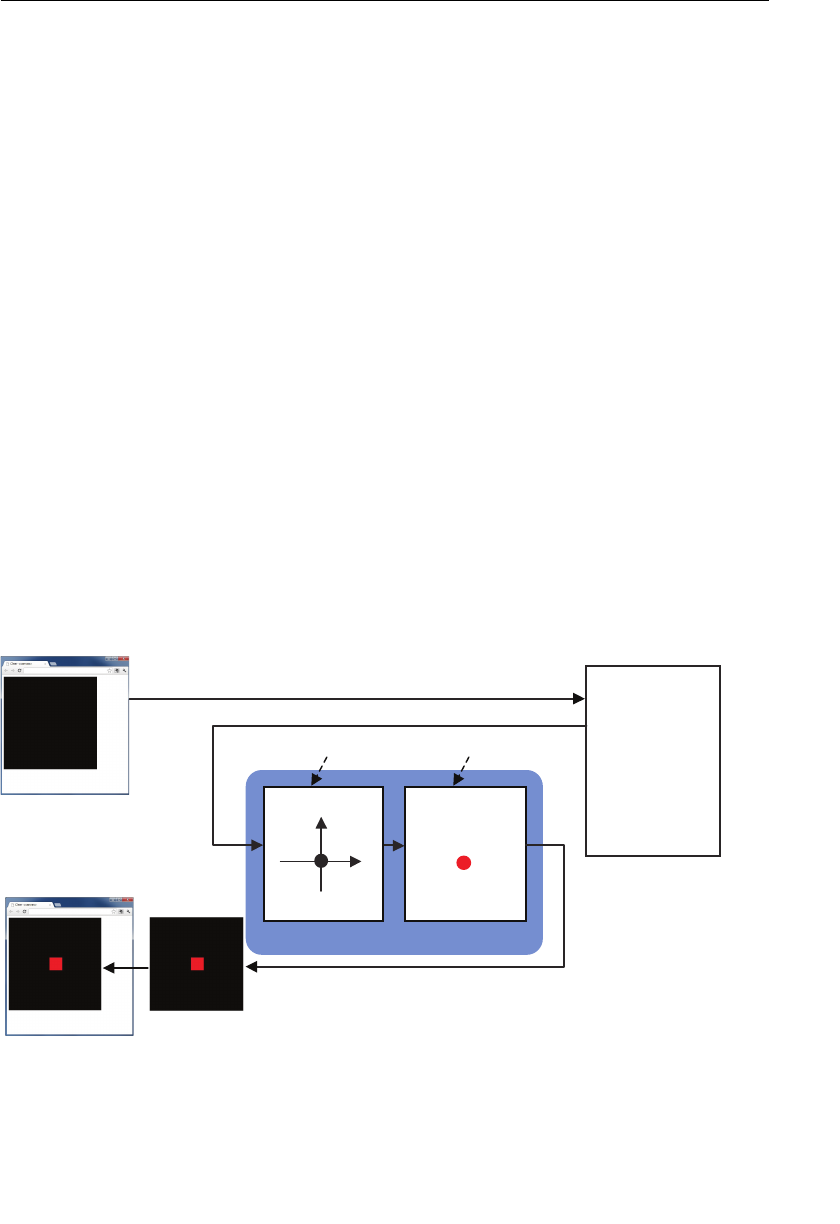
ptg11539634

Draw a Point (Version 1) 27

What Is a Shader?

HelloPoint1.js is our first WebGL program that uses shaders. As mentioned earlier,

shader programs are necessary when you want to draw something on the screen in

WebGL. Essentially, shader programs are “embedded” in the JavaScript file and, in this

case, set up at the start. This seems at first sight to be complicated, but let’s take it one

step at a time.

WebGL needs the following two types of shaders, which you saw at line 2 and line 9:

• Vertex shader: Vertex shaders are programs that describe the traits (position, colors,

and so on) of a vertex. The vertex is a point in 2D/3D space, such as the corner or

intersection of a 2D/3D shape.

• Fragment shader: A program that deals with per-fragment processing such as light-

ing (see Chapter 8 , “Lighting Objects”). The fragment is a WebGL term that you can

consider as a kind of pixel (picture element).

You’ll explore shaders in more detail later, but simply put, in a 3D scene, it’s not enough

just to draw graphics. You have to also account for how they are viewed as light sources

hit them or the viewer’s perspective changes. Shading does this with a high degree of flex-

ibility and is part of the reason that today’s 3D graphics are so realistic, allowing them to

use new rendering effects to achieve stunning results.

The shaders are read from the JavaScript and stored in the WebGL system ready to be used

for drawing. Figure 2.10 shows the basic processing flow from a JavaScript program into

the WebGL system, which applies the shader programs to draw shapes that the browser

finally displays.

metsyS LGbeW

redahS xetreV tnemgarF

redahS

tpircSavaJ

{ )(niam noitcnuf

…LGbeWteg=lg rav

…

;)…(sredahStini

…

}

noitarepo tnemgarf—rePnoitarepo xetrev—reP

resworB

:noitisoP

)0.1 ,0.0 ,0.0 ,0.0(

0.01 :eziS

:roloC

)0.1 ,0.0 ,0.0 ,0.1(

)daolno( detucexe si margorp tpircSavaJ

reffub roloc eht ot redneR

detucexe era sdohtem detaler—LGbeW

reffuB roloC

yalpsiD

Figure 2.10 The processing flow from executing a JavaScript program to displaying the result

in a browser

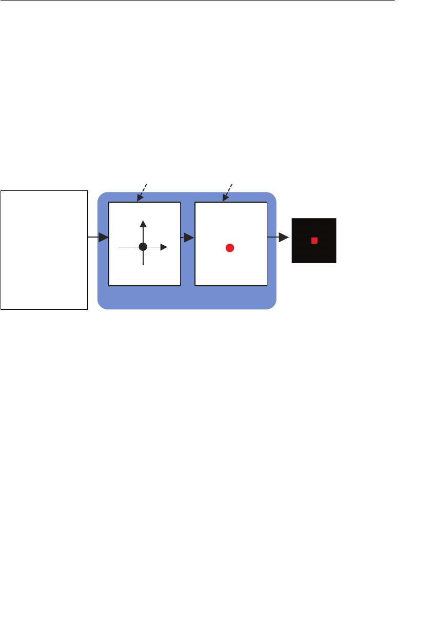
ptg11539634

CHAPTER 2 Your First Step with WebGL

You can see two browser windows on the left side of the figure. These are the same; the

upper one shows the browser before executing the JavaScript program, and the lower one

shows the browser after execution. Once the WebGL-related methods are called from the

JavaScript program, the vertex shader in the WebGL system is executed, and the fragment

shader is executed to draw the result into the color buffer. This is the clear part—that is,

step 4 in Figure 2.8 , described in the original

HelloCanvas example. Then the content in

the color buffer is automatically displayed on the drawing area specified by the

in the browser.

You’ll be seeing this figure frequently in the rest of this book. So we’ll use a simplified

version to save space (see Figure 2.11 ). Note that the flow is left to right and the right-

most component is a color buffer, not a browser, because the color buffer is automatically

displayed in the browser.

m e t s y S L G b e W

r e d a h S x e t r e V t n e m g a r F

r e d a h S

n o i t a r e p o t n e m g a r

— r e P n o i t a r e p o x e t r e v — r e P

: n o i t i s o

) 0 . 1

0 . 0 , 0 . 0 , 0 . 0 (

0 . 0 1 : e z i S

: r o l o C

) 0 . 1 , 0 . 0 , 0 . 0 , 0 . 1 ( r e f f u B r o l o C

t p i r c S a v a J

{ ) ( n i a m n o i t c n u f

… L G b e W t e g = l g r a v

…

; ) … ( s r e d a h S t i n i

…

}

Figure 2.11 The simplified version of Figure 2.9

Getting back to our example, the goal is to draw a 10-pixel point on the screen. The two

shaders are used as follows:

• The vertex shader specifies the position of a point and its size. In this sample

program, the position is (0.0, 0.0, 0.0), and the size is 10.0.

• The fragment shader specifies the color of fragments displaying the point. In this

sample program, the color is red (1.0, 0.0, 0.0, 1.0).

The Structure of a WebGL Program that Uses Shaders

Based on what you’ve learned so far, let’s look at HelloPoint1.js again (refer to Listing

2.5 ). This program has 40 lines and is a little more complex than

HelloCanvas.js (18

lines). It consists of three parts, as shown in Figure 2.12 . The

main() function in JavaScript

starts from line 15, and shader programs are located from lines 2 to 13.

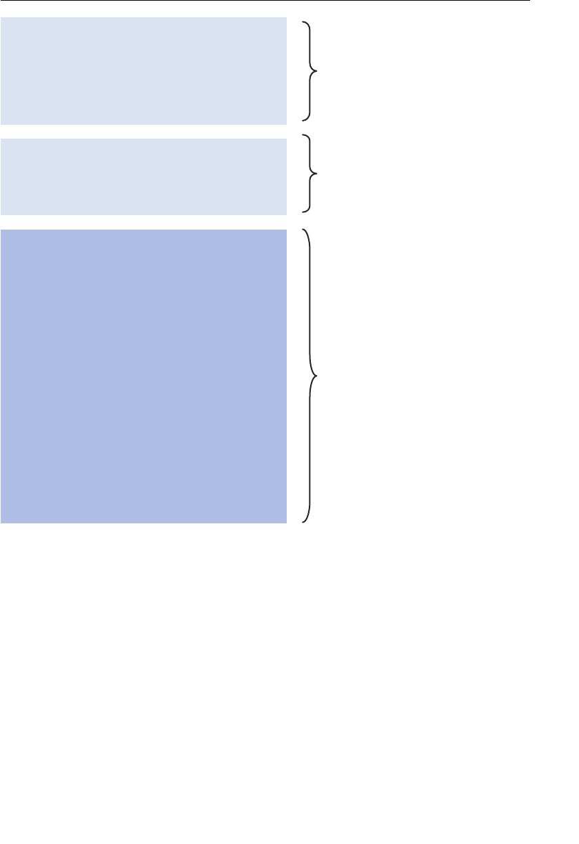
ptg11539634

Draw a Point (Version 1) 29

sj.1tniPolleH//1

margorpredahsxetreV//2

=ECRUOS_REDAHSVrav3

+‘n{)(niamdiov‘4

+‘n;)0.1,0.0,0.0,0.0(4cev=noitisoP_lg‘5

+‘n;0.01=eziStnioP_lg‘6

;‘n}‘7

margorpredahstnemgarF//9

=ECRUOS_REDAHSFrav01

+‘n{)(niamd

iov‘11

+‘n;)0.1,0.0,0.0,0.1(4cev=roloCgarF_lg‘21

;‘n}‘31

{)(niamnoitcnuf51

tnemele>savnac<eveirteR//6

;)‘lgbew‘(dIyBtnemelEteg.tnemucod=savnacrav71

LGbeWroftxetnocgnirednerehtteG//91

;)savnac(txetnoCLGbeWteg=lgrav02

…

sredahsezilaitinI//62

…,ECRUOS_REDAHSV,lg(sredahStini!(fi72

…

>savnac<gniraelcrofrolocehtteS//23

;)0.1,0.0,0.0,0.0(roloCraelc.lg33

…

>savnac<raelC//53

;)TIB_REFFUB_ROLOC.lg(raelc.lg63

tniopawarD

//83

;)1,0,STNIOP.lg(syarrAward.lg93

}04

Vertex shader program

(Language: GLSL ES)

Fragment shader program

(Language: GLSL ES)

Main program

(Language: JavaScript)

Figure 2.12 The basic structure of a WebGL program with embedded shader programs

The vertex shader program is located in lines 4 to 7, and the fragment shader is located in

lines 11 to 13. These programs are actually the following shader language programs but

written as a JavaScript string to make it possible to pass the shaders to the WebGL system:

// Vertex shader program

void main() {

gl_Position = vec4(0.0, 0.0, 0.0, 1.0);

gl_PointSize = 10.0;

}

// Fragment shader program

void main() {

gl_FragColor = vec4(1.0, 0.0, 0.0, 1.0);

}

ptg11539634

CHAPTER 2 Your First Step with WebGL

As you learned in Chapter 1 , shader programs must be written in the OpenGL ES shading

language (GLSL ES) , which is similar to the C language. Finally, GLSL ES comes onto the

stage! You will get to see the details of GLSL ES in Chapter 6 , “The OpenGL ES Shading

Language (GLSL ES),” but in these early examples, the code is simple and should be under-

standable by anybody with a basic understanding of C or JavaScript.

Because these programs must be treated as a single string, each line of the shader is

concatenated using the

+ operator into a single string. Each line has n at the end because

the line number is displayed when an error occurs in the shader. The line number is

helpful to check the source of the problem in the codes. However, the

n is not manda-

tory, and you could write the shader without it.

At lines 3 and 10, each shader program is stored in the variables

VSHADER_SOURCE and

FSHADER_SOURCE as a string:

2 // Vertex shader program

3 var VSHADER_SOURCE =

4 ‘void main() {n’ +

5 ‘ gl_Position = vec4(0.0, 0.0, 0.0, 1.0);n’ +

6 ‘ gl_PointSize = 10.0;n’ +

7 ‘}n’;

9 // Fragment shader program

10 var FSHADER_SOURCE =

11 ‘void main() {n’ +

12 ‘ gl_FragColor = vec4(1.0, 0.0, 0.0, 1.0);n’ +

13 ‘}n’;

If you are interested in loading the shader programs from files, refer to Appendix F ,

“Loading Shader Programs from Files.”

Initializing Shaders

Before looking at the details of each shader, let’s examine the processing flow of main()

that is defined from line 15 in the JavaScript (see Figure 2.13 ). This flow, shown in Figure

2.13 , is the basic processing flow of most WebGL applications. You will see the same flow

throughout this book.

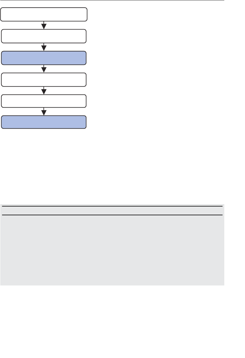
ptg11539634

Draw a Point (Version 1) 31

LGbeWroftxetnocgnirednerehtteG

>savnac<raelC

sredahsezilaitinI

warD

tnemele>savnac<ehteveirteR

>savnac<gniraelcrofrolocehtteS

Figure 2.13 The processing flow of a WebGL program

This flow is similar to that shown in Figure 2.8 except that a third step (“Initialize

Shaders”) and a sixth step (“Draw”) are added.

The third step “Initialize Shaders” initializes and sets up the shaders that are defined at

line 3 and line 10 within the WebGL system. This step is done using the convenience

function

initShaders() that is defined in cuon-util.js . Again, this is one of those special

functions we have provided for this book.

initShaders(gl, vshader, fshader)

Initialize shaders and set them up in the WebGL system ready for use:

Parameters gl Specifies a rendering context.

vshader Specifies a vertex shader program (string).

fshader Specifies a fragment shader program (string).

Return value true Shaders successfully initialized.

false Failed to initialize shaders.

Figure 2.14 shows how the convenience function

initShaders() processes the shaders.

You will examine in detail what this function is doing in Chapter 8 . For now, you just

need to understand that it sets up the shaders in the WebGL system and makes them

ready for use.

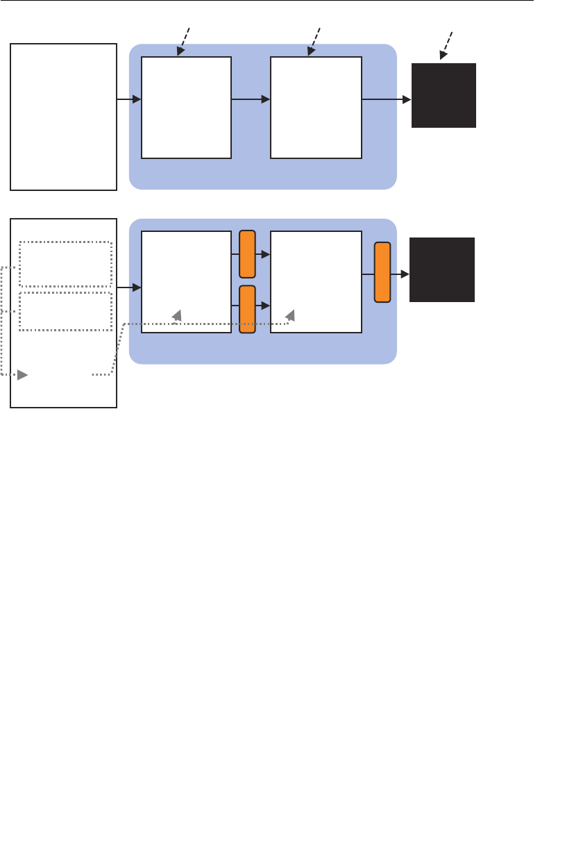
ptg11539634

CHAPTER 2 Your First Step with WebGL

metsySLGbeW

redahSxet

reV tnemgarF

redahS

noitarepotnemgarf—rePnoitarepoxetrev—reP r

fuBr

loC

tpirc

avaJ

redahSxetreV tnemgarF

redahS

gl_Position

gl_PointSize

gl_FragColor

{)(niamdiov

;)...(4cev=noitisoP_lg

;0.01=eziStnioP_lg

}

{)(niamdiov

;)...(4cev=roloCgarF_lg

}

tpircSavaJ

{)(niamd

iov

;)...(4cev=noitisoP_lg

;0.01=eziStnioP_lg

}

{)(niamdiov

;)...(4cev=rolo

garF_lg

}

{)(niamnoitcnu

…LGbeWteg=lgrav

…

;)…(sredahStini

…

}

Figure 2.14 Behavior of initShaders()

As you can see in the upper figure in Figure 2.14 , the WebGL system has two containers:

one for a vertex shader and one for a fragment shader. This is actually a simplification,

but helpful at this stage. We return to the details in Chapter 10 . By default, the contents

of these containers are empty. To make the shader programs, written as JavaScript strings

and ready for use in the WebGL system, we need something to pass these strings to the

system and then set them up in the appropriate containers;

initShaders() performs this

operation. Note that the shader programs are executed within the WebGL system, not the

JavaScript program.

The lower portion in Figure 2.14 shows that after executing

initShaders() , the shader

programs that are passed as a string to the parameters of

initShaders() are set up in the

containers in the WebGL system and then made ready for use. The lower figure schemati-

cally illustrates that a vertex shader is passing

gl_Position and gl_PointSize to a frag-

ment shader and that just after assigning values to these variables in the vertex shader, the

fragment shader is executed. In actuality, the fragments that are generated after process-

ing these values are passed to the fragment shader. Chapter 5 explains this mechanism in

detail, but for now you can consider the attributes to be passed.

ptg11539634

Draw a Point (Version 1) 33

The important point here is that WebGL applications consist of a JavaScript program executed

by the browser and shader programs that are executed within the WebGL system .

Now, having completed the explanation of the second step “Initialize Shaders” in Figure

2.13 , you are ready to see how the shaders are actually used to draw a simple point. As

mentioned, we need three items of information for the point: its position, size, and color,

which are used as follows:

• The vertex shader specifies the position of a point and its size. In this sample

program, the position is (0.0, 0.0, 0.0), and the size is 10.0.

• The fragment shader specifies the color of the fragments displaying the point. In this

sample program, they are red (1.0, 0.0, 0.0, 1.0).

Vertex Shader

Now, let us start by examining the vertex shader program listed in HelloPoint1.js (refer

to Listing 2.5 ), which sets the position and size of the point:

2 // Vertex shader program

3 var VSHADER_SOURCE =

4 ‘void main() {n’ +

5 ‘ gl_Position = vec4(0.0, 0.0, 0.0, 1.0);n’ +

6 ‘ gl_PointSize = 10.0;n’ +

7 ‘}n’;

The vertex shader program itself starts from line 4 and must contain a single main() func-

tion in a similar fashion to languages such as C. The keyword

void in front of main()

indicates that this function does not return a value. You cannot specify other arguments

main() .

Just like JavaScript, we can use the = operator to assign a value to a variable in a shader.

Line 5 assigns the position of the point to the variable

gl_Position , and line 6 assigns its

size to the variable

gl_PointSize . These two variables are built-in variables available only

in a vertex shader and have a special meaning:

gl_Position specifies a position of a vertex

(in this case, the position of the point), and

gl_PointSize specifies the size of the point

(see Table 2.2 ).

Table 2.2 Built-In Variables Available in a Vertex Shader

Type and Variable Name Description

vec4

gl_Position Specifies the position of a vertex

float

gl_PointSize Specifies the size of a point (in pixels)

ptg11539634

CHAPTER 2 Your First Step with WebGL

Note that gl_Position should always be written. If you don’t specify it, the shader’s

behavior is implementation dependent and may not work as expected. In contrast,

gl_

PointSize is only required when drawing points and defaults to a point size of 1.0 if you

don’t specify anything.

For those of you mostly familiar with JavaScript, you may be a little surprised when you

see “type” specified in Table 2.2 . Unlike JavaScript, GLSL ES is a “typed” programming

language; that is, it requires the programmer to specify what type of data a variable holds.

C and Java are examples of typed languages. By specifying “type” for a variable, the

system can easily understand what type of data the variable holds, and then it can opti-

mize its processing based on that information. Table 2.3 summarizes the “type” in GLSL

ES used in the shaders in this section.

Table 2.3 Data Types in GLSL ES

Type Description

float Indicates a floating point number

vec4 Indicates a vector of four floating point numbers

float float Float float

Note that an error will occur when the type of data that is assigned to the variable is

different from the type of the variable. For example, the type of

gl_PointSize is float, and

you must assign a floating point number to it. So, if you change line 6 from

gl_PointSize = 10.0;

gl_PointSize = 10;

it will generate an error simply because 10 is interpreted as an integer number, whereas

10.0 is a floating point number in GLSL ES.

The type of the variable gl_Position , the built-in variable for specifying the position of

a point, is

vec4 ; vec4 is a vector made up of three floats. However, you only have three

floats (0.0, 0.0, 0.0) representing X, Y, and Z. So you need to convert these to a

vec4

somehow. Fortunately, there is a built-in function,

vec4() , that will do this for you and

return a value of type

vec4 –, which is just what you need!

ptg11539634

Draw a Point (Version 1) 35

vec4 vec4(v0, v1, v2, v3)

Construct a

vec4 object from v0 , v1 , v2 , and v3 .

Parameters v0, v1, v2, v3 Specifies floating point numbers.

Return value A

vec4 object made from v0 , v1 , v2 , and v3.

In this sample program,

vec4() is used at line 5 as follows:

gl_Position = vec4(0.0, 0.0, 0.0, 1.0);

Note that the value that is assigned to gl_Position has 1.0 added as a fourth component.

This four-component coordinate is called a homogeneous coordinate (see the boxed

article below) and is often used in 3D graphics for processing three-dimensional informa-

tion efficiently. Although the homogeneous coordinate is a four-dimensional coordinate,

if the last component of the homogeneous coordinate is 1.0, the coordinate indicates the

same position as a three-dimensional one. So, you can supply 1.0 as the last component if

you need to specify four components as a vertex coordinate.

Homogeneous Coordinates

The homogeneous coordinates use the following coordinate notation: (x, y, z, w). The

homogeneous coordinate (x, y, z, w) is equivalent to the three-dimensional coordinate

(x/w, y/w, z/w). So, if you set w to 1.0, you can utilize the homogeneous coordinate

as a three-dimensional coordinate. The value of w must be greater than or equal to

0. If w approaches zero, the coordinates approach infinity. So we can represent the

concept of infinity in the homogeneous coordinate system. Homogeneous coordinates

make it possible to represent vertex transformations described in the next chapter as a

multiplication of a matrix and the coordinates. These coordinates are often used as an

internal representation of a vertex in 3D graphics systems.

Fragment Shader

After specifying the position and size of a point, you need to specify its color using a frag-

ment shader. As explained earlier, a fragment is a pixel displayed on the screen, although

technically the fragment is a pixel along with its position, color, and other information.

The fragment shader is a program that processes this information in preparation for

displaying the fragment on the screen. Looking again at the fragment shader listed in

HelloPoint1.js (refer to Listing 2.5 ), you can see that just like a vertex shader, a fragment

shader is executed from

main() :

ptg11539634

CHAPTER 2 Your First Step with WebGL

9 // Fragment shader program

10 var FSHADER_SOURCE =

11 ‘void main() {n’ +

12 ‘ gl_FragColor = vec4(1.0, 0.0, 0.0, 1.0);n’ +

13 ‘}n’;

The job of the shader is to set the color of the point as its per-fragment operation, which

is carried out at line 12.

gl_FragColor is a built-in variable only available in a fragment

shader; it controls the color of a fragment, as shown in Table 2.4 .

Table 2.4 The Built-In Value Available in a Fragment Shader

Type and Variable Name Description

vec4

gl_FragColor Specify the color of a fragment (in RGBA)

When we assign a color value to the built-in variable, the fragment is displayed using

that color. Just like the position in the vertex shader, the color value is a

vec4 data type

consisting of four floating point numbers representing the RGBA values. In this sample

program, a red point will be displayed because you assign (1.0, 0.0, 0.0, 1.0) to the

variable.

The Draw Operation

Once you set up the shaders, the remaining task is to draw the shape, or in our case, a

point. As before, you need to clear the drawing area in a similar way to that described

HelloCanvas.js . Once the drawing area is cleared, you can draw the point using gl.

drawArrays() , as in line 39:

39 gl.drawArrays(gl.POINTS, 0, 1);

gl.drawArrays() is a powerful function that is capable of drawing a variety of basic

shapes, as detailed in the following box.

ptg11539634

Draw a Point (Version 1) 37

gl.drawArrays(mode, first, count)

Execute a vertex shader to draw shapes specified by the mode parameter.

Parameters mode Specifies the type of shape to be drawn. The following symbolic

constants are accepted:

gl.POINTS , gl.LINES , gl.LINE_STRIP ,

gl.LINE_LOOP , gl.TRIANGLES , gl.TRIANGLE_STRIP , and gl.

TRIANGLE_FAN.

first Specifies which vertex to start drawing from (integer).

count Specifies the number of vertices to be used (integer).

Return value None

Errors INVALID_ENUM mode is none of the preceding values.

INVALID_VALUE first is negative or count is negative.

In this sample program, because you are drawing a point, you specify

gl.POINTS as the

mode in the first parameter. The second parameter is set to 0 because you are starting from

the first vertex. The third parameter, count , is 1 because you are only drawing 1 point in

this sample program.

Now, when the program makes a call to

gl.drawArrays() , the vertex shader is executed

count times, each time working with the next vertex. In this sample program, the shader

is executed once ( count is set to 1) because we only have one vertex: our point. When

the shader is executed, the function

main() in the shader is called, and then each line

in the function is executed sequentially, resulting in (0.0, 0.0, 0.0, 1.0) being assigned to

gl_Position (line 5) and then 10.0 assigned to gl_PointSize (line 6).

Once the vertex shader executes, the fragment shader is executed by calling its main()

function which, in this example, assigns the color value (red) to

gl_FragColor (line 12).

As a result, a red point of 10 pixels is drawn at (0.0, 0.0, 0.0, 1.0), or the center of the

drawing area (see Figure 2.15 ).

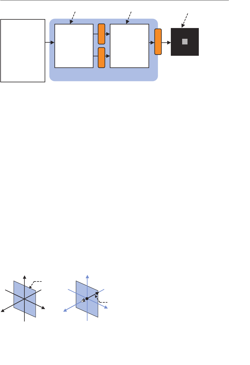
ptg11539634

CHAPTER 2 Your First Step with WebGL

metsySLGbeW

r e d a h S x e t r e V t n e m g a r F

r e d a h S

o i t

a r e p o t n e m g a r f — r e P n o i t a r e p o x e t r e v — r e P r e f f u B r o l o C

gl_PointSize

{)(niamdiov

=noitisoP_lg

;)0.1,0.0,0.0,0.0(4cev

;0.01=eziStni

oP_lg

}

gl_FragColor

t p i r c S a v a J

{ ) ( n i a m n o i t c n u f

… L G b e W t e g = l g r a v

…

;

)

… ( s r e d a h S t i n i

…

; ) … ( s y a r r A w a r d . l g

}

gl_Position

{)(niamdiov

=rol

oCgarF_lg

;)

0.1,0.

0,0.0,0.1(4cev

}

Figure 2.15 The behavior of shaders

At this stage, you should have a rough understanding of the role of a vertex shader and a

fragment shader and how they work. In the rest of this chapter, you’ll build on this basic

understanding through a series of examples, allowing you to become more accustomed to

WebGL and shaders. However, before that, let’s quickly look at how WebGL describes the

position of shapes using its coordinate system.

The WebGL Coordinate System

Because WebGL deals with 3D graphics, it uses a three-dimensional coordinate system

along the x-, y-, and z-axis. This coordinate system is easy to understand because our

world has the same three dimensions: width, height, and depth. In any coordinate system,

the direction of each axis is important. Generally, in WebGL, when you face the computer

screen, the horizontal direction is the x-axis (right direction is positive), the vertical direc-

tion is the y-axis (up direction is positive), and the direction from the screen to the viewer

is the z-axis (the left side of Figure 2.16 ). The viewer’s eye is located at the origin (0.0, 0.0,

0.0), and the line of sight travels along the negative direction of the z-axis, or from you

into the screen (see the right side of Figure 2.16 ). This coordinate system is also called the

right-handed coordinate system because it can be expressed using the right hand (see

Figure 2.17 ) and is the one normally associated with WebGL. Throughout this book, we’ll

use the right-handed coordinate system as the default for WebGL. However, you should

note that it’s actually more complex than this. In fact, WebGL is neither left handed nor

right handed. This is explained in detail in Appendix D , “WebGL/OpenGL: Left or Right

Handed?,” but it’s safe to treat WebGL as right handed for now.

neercS

thgisfoeniL

Figure 2.16 WebGL coordinate system

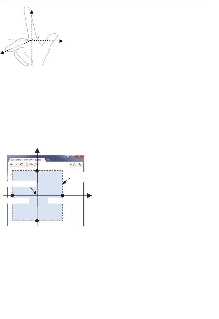
ptg11539634

Draw a Point (Version 1) 39

Figure 2.17 The right-handed coordinate system

As you have already seen, the drawing area specified for a

<canvas> element in JavaScript

is different from WebGL’s coordinate system, so a mapping is needed between the two.

By default, as you see in Figure 2.18 , WebGL maps the coordinate system to the area as

follows:

• The center position of a <canvas> : (0.0, 0.0, 0.0)

• The two edges of the x-axis of the <canvas> : (–1.0, 0.0, 0.0) and (1.0, 0.0, 0.0)

• The two edges of the y-axis of the <canvas> : (0.0, –1.0, 0.0) and (0.0, 1.0, 0.0)

(-1.0, 0.0, 0.0) (1.0, 0.0, 0.0)

(0.0, 0.0, 0.0)

(0.0, -1.0, 0.0)

drawing area

Figure 2.18 The <canvas> drawing area and WebGL coordinate system

As previously discussed, this is the default. It’s possible to use another coordinate

system, which we’ll discuss later, but for now this default coordinate system will be used.

Additionally, to help you stay focused on the core functionality of WebGL, the example

programs will mainly use the x and y coordinates and not use the z or depth coordinate.

Therefore, until Chapter 7 , the z-axis value will generally be specified as 0.0.

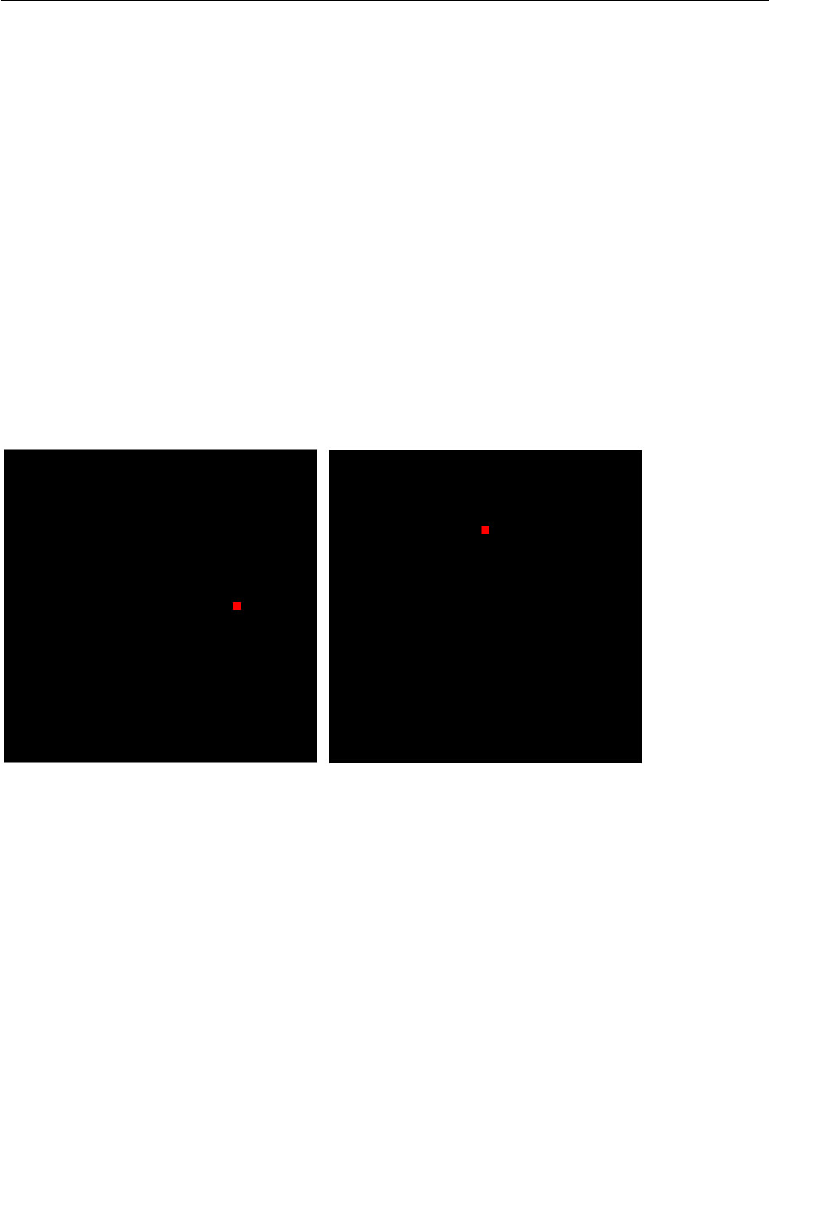
ptg11539634

CHAPTER 2 Your First Step with WebGL

Experimenting with the Sample Program

First, you can modify line 5 to change the position of the point and gain a better under-

standing of the WebGL coordinate system. For example, let’s change the x coordinate

from 0.0 to 0.5 as follows:

5 ‘ gl_Position = vec4( 0.5 , 0.0, 0.0, 1.0);n’ +

Save the modified HelloPoint1.js and click the Reload button on your browser to reload

it. You will see that the point has moved and is now displayed on the right side of the

<canvas> area (see Figure 2.19 , left side).

Now change the y coordinate to move the point toward the top of the <canvas> as

follows:

5 ‘ gl_Position = vec4(0.0, 0.5 , 0.0, 1.0);n’ +

Again, save the modified HelloPoint1.js and reload it. This time, you can see the point

has moved and is displayed in the upper part of the canvas (see Figure 2.19 , right side).

Figure 2.19 Modifying the position of the point

As another experiment, let’s try changing the color of the point from red to green by

modifying line 12, as follows:

12 ‘ gl_FragColor = vec4(0.0, 1.0 , 0.0, 1.0);n’ +

Let’s conclude this section with a quick recap. You’ve been introduced to the two basic

shaders we use in WebGL—the vertex shader and the fragment shader—and seen how,

although they use their own language, they can be executed from within JavaScript.

You’ve also seen that the basic processing flow of a WebGL application using shaders is

the same as in other types of WebGL applications. A key lesson from this section is that

a WebGL program consists of a JavaScript program executing in conjunction with shader

programs.

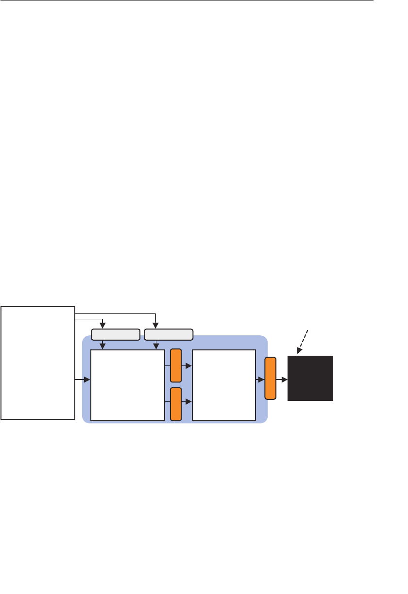
ptg11539634

Draw a Point (Version 2) 41

For those of you with experience in using OpenGL, you may feel that something is

missing; there is no code to swap color buffers. One of the significant features of WebGL

is that it does not need to do that. For more information, see Appendix A , “No Need to

Swap Buffers in WebGL.”

Draw a Point (Version 2)

In the previous section, you explored drawing a point and the related core functions of

shaders. Now that you understand the fundamental behavior of a WebGL program, let’s

examine how to pass data between JavaScript and the shaders.

HelloPoint1 always draws

a point at the same position because its position is directly written (“hard-coded”) in the

vertex shader. This makes the example easy to understand, but it lacks flexibility. In this

section, you’ll see how a WebGL program can pass a vertex position from JavaScript to

the vertex shader and then draw a point at that position. The name of the program is

HelloPoint2 , and although the result of the program is the same as HelloPoint1 , it’s a

flexible technique you will use in future examples.

Using Attribute Variables

Our goal is to pass a position from the JavaScript program to the vertex shader. There

are two ways to pass data to a vertex shader: attribute variable and uniform variable (see

Figure 2.20 ). The one you use depends on the nature of the data. The attribute variable

passes data that differs for each vertex, whereas the uniform variable passes data that is

the same (or uniform) in each vertex. In this program, you will use the attribute variable

because each vertex generally has different coordinates.

r e d a h S x

e t r e V t n e m g a r F

r e d a h S

gl_Position gl_PointSize

gl_FragColor

e l b a i r a v

e t u b i r t t a e l b a i r a v m r o f i n u

t p i r c S a v a J

{ ) ( n i a m n o i t c n u f

… L G b e W t e g = l g r a v

…

; ) … ( s r

e d a h S t i

n i

…

}

r e f f u B r o l o C

m e t s y S L G b e W

Figure 2.20 Two ways to pass data to a vertex shader

The attribute variable is a GLSL ES variable which is used to pass data from the world

outside a vertex shader into the shader and is only available to vertex shaders.

ptg11539634

CHAPTER 2 Your First Step with WebGL

To use the attribute variable, the sample program involves the following three steps:

1. Prepare the attribute variable for the vertex position in the vertex shader.

2. Assign the attribute variable to the

gl_Position variable.

3. Pass the data to the attribute variable.

Let’s look at the sample program in more detail to see how to carry out these steps.

Sample Program (HelloPoint2.js)

In HelloPoint2 (see Listing 2.6 ), you draw a point at a position the JavaScript program

specifies.

Listing 2.6 HelloPoint2.js

1 // HelloPoint2.js

2 // Vertex shader program

3 var VSHADER_SOURCE =

4 ‘attribute vec4 a_Position;n’ +

5 ‘void main() {n’ +

6 ‘ gl_Position = a_Position;n’ +

7 ‘ gl_PointSize = 10.0;n’ +

8 ‘}n’;

10 // Fragment shader program

… snipped because it is the same as HelloPoint1.js

16 function main() {

17 // Retrieve <canvas> element

18 var canvas = document.getElementById(‘webgl’);

20 // Get the rendering context for WebGL

21 var gl = getWebGLContext(canvas);

…

27 // Initialize shaders

28 if (!initShaders(gl, VSHADER_SOURCE, FSHADER_SOURCE)) {

…

31 }

33 // Get the storage location of attribute variable

34 var a_Position = gl.getAttribLocation(gl.program, ‘a_Position’);

35 if (a_Position < 0) {

36 console.log(‘Failed to get the storage location of a_Position’);

37 return;

ptg11539634

Draw a Point (Version 2) 43

38 }

40 // Pass vertex position to attribute variable

41 gl.vertexAttrib3f(a_Position, 0.0, 0.0, 0.0);

43 // Set the color for clearing <canvas>

44 gl.clearColor(0.0, 0.0, 0.0, 1.0);

46 // Clear <canvas>

47 gl.clear(gl.COLOR_BUFFER_BIT);

49 // Draw a point

50 gl.drawArrays(gl.POINTS, 0, 1);

51 }

As you can see, the attribute variable is prepared within the shader on line 4:

4 ‘attribute vec4 a_Position;n’ +

In this line, the keyword attribute is called a storage qualifier , and it indicates that the

following variable (in this case,

a_Position ) is an attribute variable. This variable must

be declared as a global variable because data is passed to it from outside the shader. The

variable must be declared following a standard pattern

<Variable Name> , as shown in Figure 2.21 .

;noitisoP_a4cevetubirtta

emaNelbairaVepyTreifilauQegarotS

Figure 2.21 The declaration of the attribute variable

In line 4, you declare

a_Position as an attribute variable with data type vec4 because,

as you saw in Table 2.2 , it will be assigned to

gl_Position , which always requires a vec4

type.

Note that throughout this book, we have adopted a programming convention in which

all attribute variables have the prefix

a_ , and all uniform variables have the prefix u_ to

easily determine the type of variables from their names. Obviously, you can use your own

convention when writing your own programs, but we find this one simple and clear.

Once

a_Position is declared, it is assigned to gl_Position at line 6:

6 ‘ gl_Position = a_Position;n’ +

At this point, you have completed the preparation in the shader for receiving data from

the outside. The next step is to pass the data to the attribute variable from the JavaScript

program.

ptg11539634

CHAPTER 2 Your First Step with WebGL

Getting the Storage Location of an Attribute Variable

As you saw previously, the vertex shader program is set up in the WebGL system using

the convenience function

initShaders() . When the vertex shader is passed to the

WebGL system, the system parses the shader, recognizes it has an attribute variable, and

then prepares the location of its attribute variable so that it can store data values when

required. When you want to pass data to

a_Position in the vertex shader, you need to

ask the WebGL system to give you the location it has prepared, which can be done using

gl.getAttribLocation() , as shown in line 34:

33 // Get the location of attribute variable

34 var a_Position = gl.getAttribLocation(gl.program, ‘a_Position’);

35 if (a_Position < 0) {

36 console.log(‘Fail to get the storage location of a_Position’);

37 return;

38 }

The first argument of this method specifies a program object that holds the vertex shader

and the fragment shader. You will examine the program object in Chapter 8 , but for

now, you can just specify

gl.program as the argument here. Note that you should use

gl.program only after initShaders() has been called because initShaders() assigns the

program object to the variable. The second parameter specifies the attribute variable name

(in this case

a_Position ) whose location you want to know.

The return value of this method is the storage location of the specified attribute variable.

This location is then stored in the JavaScript variable,

a_Position , at line 34 for later use.

Again, for ease of understanding, this book uses JavaScript variable names for attribute

variables, which are the same as the GLSL ES attribute variable name. You can, of course,

use any variable name.

The specification of

gl.getAttribLocation() is as follows:

gl.getAttribLocation(program, name)

Retrieve the storage location of the attribute variable specified by the name parameter.

Parameters program Specifies the program object that holds a vertex

shader and a fragment shader.

name Specifies the name of the attribute variable

whose location is to be retrieved.

Return value greater than or equal to 0 The location of the specified attribute variable.

-1 The specified attribute variable does not exist or

its name starts with the reserved prefix

gl_ or

webgl_ .

ptg11539634

Draw a Point (Version 2) 45

Errors INVALID_OPERATION program has not been successfully linked (See

Chapter 9 .)

INVALID_VALUE The length of name is more than the maximum

length (256 by default) of an attribute variable

name.

Assigning a Value to an Attribute Variable

Once you have the attribute variable location, you need to set the value using the

a_Position variable. This is performed at line 41 using the gl.vertexAttrib3f() method.

40 // Set vertex position to attribute variable

41 gl.vertexAttrib3f(a_Position, 0.0, 0.0, 0.0);

The following is the specification of gl.vertexAtrrib3f() .

gl.vertexAttrib3f(location, v0, v1, v2)

Assign the data ( v0 , v1 , and v2 ) to the attribute variable specified by location .

Parameters location Specifies the storage location of an attribute variable to be modified.

v0 Specifies the value to be used as the first element for the attribute

variable.

v1 Specifies the value to be used as the second element for the attri-

bute variable.

v2 Specifies the value to be used as the third element for the attribute

variable.

Return value None

Errors INVALID_OPERATION There is no current program object.

INVALID_VALUE location is greater than or equal to the maximum

number of attribute variables (8, by default).

The first argument of the method call specifies the location returned by

gl.getAttrib-

Location() at line 34. The second, third, and fourth arguments specify the floating point

number to be passed to

a_Position representing the x, y, and z coordinates of the point.

After calling the method, these three values are passed as a group to

a_Position , which

was prepared at line 4 in the vertex shader. Figure 2.22 shows the processing flow of

getting the location of the attribute variable and then writing a value to it.

ptg11539634

CHAPTER 2 Your First Step with WebGL

metsySLGbeW

gl_Position

gl_PointSize

tpircSavaJ

redahSxetreV

{)(niamdiov

;noitisoP_a=noitisoP_lg

;0.01=eziStnioP_lg

}

{)(niamnoitcnuf

;)(txetnoCLGbeWteg=lgrav

…

;)…,ECRU

OS_REDAHSV,lg(sredahStini

=noitisoP_a

;)’noitisoP_a‘,…(noitacoLetubirttAteg.lg

…

P_a(f3etubirttAxetrev.lg;)0.0,0.0,0.0,noitiso

…

}

metsySLGbeW

gl_Position

gl_PointSize

tpircSavaJ

redahSxetreV

{)(niamdiov

;noitisoP_a=noitisoP_lg

;0.01=eziStnioP_

}

{)(niamnoi

tcn

;)(txetnoCLGbeWteg=lgrav

…

;)…,ECRU

OS_REDAHSV,lg(sredahStini

=noitisoP_a

;)’

noitisoP

_a‘,…(noitacoLetub

irttAteg.lg

…

P_a(f3etubirttAxetrev.lg ;)0.0,0.0,0.0,noitiso

…

}

noitisoP_a

Figure 2.22 Getting the storage location of an attribute variable and then writing a value to

the variable

a_Position is then assigned to gl_Position at line 6 in the vertex shader, in effect passing

the x, y, and z coordinates from your JavaScript, via the attribute variable into the shader,

where it’s written to

gl_Position . So the program has the same effect as HelloPoint1 ,

where

gl_Position is used as the position of a point. However, gl_Position has now been

set dynamically from JavaScript rather than statically in the vertex shader:

4 ‘attribute vec4 a_Position;n’ +

5 ‘void main() {n’ +

6 ‘ gl_Position = a_Position;n’ +

7 ‘ gl_PointSize = 10.0;n’ +

8 ‘}n’;

Finally, you clear the <canvas> using gl.clear() (line 47) and draw the point using

gl.drawArrays() (line 50) in the same way as in HelloPoint1.js .

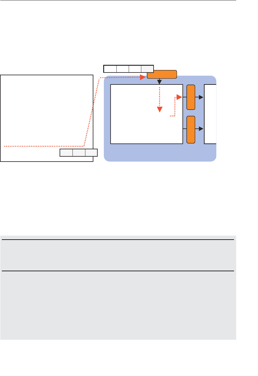
ptg11539634

Draw a Point (Version 2) 47

As a final note, you can see a_Position is prepared as vec4 at line 4 in the vertex shader.

However,

gl.vertexAttrib3f() at line 41 specifies only three values (x, y, and z), not

four. Although you may think that one value is missing, this method automatically

supplies the value 1.0 as the fourth value (see Figure 2.23 ). As you saw earlier, a default

fourth value of 1.0 for a color ensures it is fully opaque, and a default fourth value of 1.0

for a homogeneous coordinate maps a 3D coordinate into a homogenous coordinate, so

essentially the method is supplying a “safe” fourth value.

metsySLGbeW

gl_Position

gl_PointSize

tpircSavaJ

redahSxetreV

{)(niamdiov

;noitisoP_a=noitisoP_lg

;0.01

=eziStnioP_lg

}

{)(niamnoitcn fu

;)(txetnoCLGbeWteg=lgrav

…

;)…,ECRUOS_REDAHSV,lg(sredahStini

=noitisoP_a

;)’noitisoP_a‘,…(noitacoLetubirttAteg.lg

…

P_a(f3etubirttAxetrev.lg;)0.0,0.0,0.0,noitiso

…

}

0.0 0.0 0.0

n o i t i s o P _ a

0 . 0 0 . 0 0 . 0 0 . 1

Figure 2.23 The missing data is automatically supplied

Family Methods of gl.vertexAttrib3f()

gl.vertexAttrib3f() is part of a family of methods that allow you to set some or all of

the components of the attribute variable.

gl.vertexAttrib1f() is used to assign a single

value (v0),

glvertexAttrib2f() assigns two values (v0 and v1), and gl.vertexAttrib4f()

assigns four values (v0, v1, v2, and v3).

gl.vertexAttrib1f(location, v0)

gl.vertexAttrib2f(location, v0, v1)

gl.vertexAttrib3f(location, v0, v1, v2)

gl.vertexAttrib4f(location, v0, v1, v2, v3)

Assign data to the attribute variable specified by location .

gl.vertexAttrib1f() indicates

that only one value is passed, and it will be used to modify the first component of the

attribute variable. The second and third components will be set to 0.0, and the fourth

component will be set to 1.0. Similarly,

gl.vertexAttrib2f() indicates that values are

provided for the first two components, the third component will be set to 0.0, and the

fourth component will be set to 1.0.

gl.vertexAttrib3f() indicates that values are

provided for the first three components, and the fourth component will be set to 1.0,

whereas

gl.vertexAttrib4f() indicates that values are provided for all four components.

ptg11539634

CHAPTER 2 Your First Step with WebGL

Parameters location Specifies the storage location of the attribute variable.

v0, v1, v2, v3 Specifies the values to be assigned to the first, second,

third, and fourth components of the attribute variable.

Return value None

Errors INVALID_VALUE location is greater than or equal to the maximum number

of attribute variables (8 by default).

The vector versions of these methods are also available. Their name contains “v” (vector),

and they take a typed array (see Chapter 4 ) as a parameter. The number in the method

name indicates the number of elements in the array. For example,

var position = new Float32Array([1.0, 2.0, 3.0, 1.0]);

gl.vertexAttrib4fv(a_Position, position);

In this case, 4 in the method name indicates that the length of the array is 4.

The Naming Rules for WebGL-Related Methods

You may be wondering what 3f in gl.vertexAttrib3f() actually means. WebGL bases

its method names on the function names in OpenGL ES 2.0, which as you now know,

is the base specification of WebGL. The function names in OpenGL comprise the three

components:

<base function name> <number of parameters> < parameter type> .

The name of each WebGL method also uses the same components:

<number of parameters> <parameter type> as shown in Figure 2.24 .

.lg birttAxetrev 3f(2v,1v,0v,noitacol )

emandohtemesab epytretemarap:

“fdnasrebmuntniopgnitaolfsetacidni”

“isrebmunregetnisetacidni”

sretemarapfor

ebmun

Figure 2.24 The naming rules of WebGL-related methods

As you can see in the example, in the case of

gl.vertexAttrib3f() , the base method

name is

vertexAttrib , the number of parameters is 3, and the parameter type is f (that

is, float or floating point number). This method is a WebGL version of the function

glVertexAttrib3f() in OpenGL. Another character for the parameter type is i, which

indicates integer. You can use the following notation to represent all methods from

gl.

vertexAttrib1f() to gl.vertexAttrib4f() : gl.vertexAttrib[1234]f() .

Where [] indicates that one of the numbers in it can be selected.

ptg11539634

Draw a Point (Version 2) 49

When v is appended to the name, the methods take an array as a parameter. In this case,

the number in the method name indicates the number of elements in the array.

var positions = new Float32Array([1.0, 2.0, 3.0, 1.0]);

gl.vertexAttrib4fv(a_Position, positions);

Experimenting with the Sample Program

Now that you have the program to pass the position of a point from a JavaScript program

to a vertex shader, let’s change that position. For example, if you wanted to display a

point at (0.5, 0.0, 0.0), you would modify the program as follows:

33 gl.vertexAttrib3f(a_Position, 0.5 , 0.0, 0.0);

You could use other family methods of gl.vertexAttrib3f() to perform the same task in

the following way:

gl.vertexAttrib1f(a_Position, 0.5);

gl.vertexAttrib2f(a_Position, 0.5, 0.0);

gl.vertexAttrib4f(a_Position, 0.5, 0.0, 0.0, 1.0);

Now that you are comfortable using attribute variables, let’s use the same approach to

change the size of the point from within your JavaScript program. In this case, you will

need a new attribute variable for passing the size to the vertex shader. Following the

naming rule used in this book, let’s use

a_PointSize . As you saw in Table 2.2 , the type of

gl_PointSize is float , so you need to prepare the variable using the same type as follows:

attribute float a_PointSize;

So, the vertex shader becomes:

2 // Vertex shader program

3 var VSHADER_SOURCE =

4 ‘attribute vec4 a_Position;n’ +

5 ‘attribute float a_PointSize; n’ +

6 ‘void main() {n’ +

7 ‘ gl_Position = a_Position;n’ +

8 ‘ gl_PointSize = a_PointSize;n’ +

9 ‘}n’;

Then, after you get the storage location of a_PointSize , to pass the size of the point to the

variable, you can use

gl.vertexAttrib1f() . Because the type of a_PointSize is float , you

can use

gl.vertexAttrib1f() as follows:

33 // Get the storage location of attribute variable

34 var a_Position = gl.getAttribLocation(gl.program, ‘a_Position’);

…

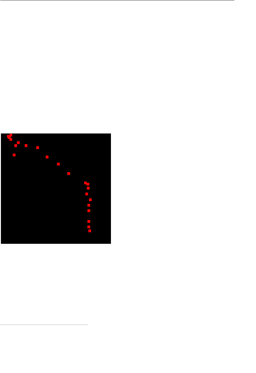
ptg11539634

CHAPTER 2 Your First Step with WebGL

39 var a_PointSize = gl.getAttribLocation(gl.program, ‘a_PointSize’);

40 // Set vertex position to attribute variable

41 gl.vertexAttrib3f(a_Position, 0.0, 0.0, 0.0);

42 gl.vertexAttrib1f(a_PointSize, 5.0);

At this stage, you might want to experiment a little with the program and make sure you

understand how to use these attribute variables and how they work.

Draw a Point with a Mouse Click

The previous program HelloPoint2 can pass the position of a point to a vertex shader

from a JavaScript program. However, the position is still hard-coded, so it is not so differ-

ent from

HelloPoint1 , in which the position was also directly written in the shader.

In this section, you add a little more flexibility, exploiting the ability to pass the position

from a JavaScript program to a vertex shader, to draw a point at the position where the

mouse is clicked. Figure 2.25 shows the screen shot of

ClickedPoint .

Figure 2.25 ClickedPoint

This program uses an event handler to handle mouse-related events, which will be famil-

iar to those of you who have written JavaScript programs.

Sample Program (ClickedPoints.js)

Listing 2.7 shows ClickedPoints.js . For brevity, we have removed code sections that are

the same as the previous example and replaced these with ….

ptg11539634

Draw a Point with a Mouse Click 51

Listing 2.7 ClickedPoints.js

1 // ClickedPoints.js

2 // Vertex shader program

3 var VSHADER_SOURCE =

4 ‘attribute vec4 a_Position;n’ +

5 ‘void main() {n’ +

6 ‘ gl_Position = a_Position;n’ +

7 ‘ gl_PointSize = 10.0;n’ +

8 ‘}n’;

10 // Fragment shader program

…

16 function main() {

17 // Retrieve <canvas> element

18 var canvas = document.getElementById(‘webgl’);

20 // Get the rendering context for WebGL

21 var gl = getWebGLContext(canvas);

…

27 // Initialize shaders

28 if (!initShaders(gl, VSHADER_SOURCE, FSHADER_SOURCE)){

…

31 }

33 // Get the storage location of a_Position variable

34 var a_Position = gl.getAttribLocation(gl.program, ‘a_Position’);

…

40 // Register function (event handler) to be called on a mouse press

41 canvas.onmousedown = function(ev) { click(ev, gl, canvas, a_Position); };

…

47 gl.clear(gl.COLOR_BUFFER_BIT);

48 }

50 var g_points = []; // The array for a mouse press

51 function click(ev, gl, canvas, a_Position) {

52 var x = ev.clientX; // x coordinate of a mouse pointer

53 var y = ev.clientY; // y coordinate of a mouse pointer

54 var rect = ev.target.getBoundingClientRect();

56 x = ((x — rect.left) — canvas.height/2)/(canvas.height/2);

57 y = (canvas.width/2 — (y — rect.top))/(canvas.width/2);

58 // Store the coordinates to g_points array

59 g_points.push(x); g_points.push(y);

ptg11539634

CHAPTER 2 Your First Step with WebGL

61 // Clear <canvas>

62 gl.clear(gl.COLOR_BUFFER_BIT);

64 var len = g_points.length;

65 for(var i = 0; i < len; i+=2) {

66 // Pass the position of a point to a_Position variable

67 gl.vertexAttrib3f(a_Position, g_points[i], g_points[i+1], 0.0);

69 // Draw a point

70 gl.drawArrays(gl.POINTS, 0, 1);

71 }

72 }

The processing flow from lines 17 to 39 is the same as HelloPoint2.js . These lines get the

WebGL context, initialize the shaders, and then retrieve the location of the attribute vari-

able. The main differences from

HelloPoint2.js are the registration of an event handler

(line 41) and the definition of the function

click() as the handler (from line 51).

An event handler is an asynchronous callback function that handles input on a web page

from a user, such as mouse clicks or key presses. This allows you to create a dynamic web

page that can change the content that’s displayed according to the user’s input. To use an

event handler, you need to register the event handler (that is, tell the system what code to

run when the event occurs). The

<canvas> supports special properties for registering event

handlers for a specific user input, which you will use here.

For example, when you want to handle mouse clicks, you can use the

onmousedown prop-

erty of the

<canvas> to specify the event handler for a mouse click as follows:

40 // Register function (event handler) to be called on a mouse press

41 canvas.onmousedown = function(ev) { click(ev, gl, canvas, a_Position); };

Line 41 uses the statement function(){ … } to register the handler:

function(ev){ click(ev, gl, canvas, a_Position); }

This mechanism is called an anonymous function , which, as its name suggests, is a

convenient mechanism when you define a function that does not need to have a name.

For those of you unfamiliar with this type of function, let’s explain the mechanism using

an example. Next, we define the variable

thanks as follows using the form:

var thanks = function () { alert(‘ Thanks a million!’); }

We can execute the variable as a function as follows:

thanks(); // ‘Thanks a million!’ is displayed

ptg11539634

Draw a Point with a Mouse Click 53

You can see that the variable thanks can be operated as a function. These lines can be

rewritten as follows:

function thanks() { alert(‘Thanks a million!’); }

thanks(); // ‘Thanks a million!’ is displayed

So why do you need to use an anonymous function? Well, when you draw a point, you

need the following three variables:

gl , canvas , and a_Position . These variables are local

variables that are prepared in the function

main() in the JavaScript program. However,

when a mouse click occurs, the browser will automatically call the function that is regis-

tered to the

<canvas> ’s onmousedown property with a predefined single parameter (that is,

an event object that contains information about the mouse press. Therefore, usually, you

will register the event handler and define the function for it as follows:

canvas.onmousedown = mousedown; // Register «mousedown» as event handler

…

function mousedown(ev) { // Event handler: It takes one parameter «ev»

…

}

However, if you define the function in this way, it cannot access the local variables gl ,

canvas , and a_Position to draw a point. The anonymous function at line 41 provides the

solution to make it possible to access them:

41 canvas.onmousedown = function(ev) { click(ev, gl, canvas, a_Position); };

In this code, when a mouse click occurs, the anonymous function function(ev) is called

first. Then it calls

click(ev, gl, canvas, a_Position) with the local variables defined

main() . Although this may seem a little complicated, it is actually quite flexible and

avoids the use of global variables, which is always good. Take a moment to make sure

you understand this approach, because you will often see this way of registering event

handlers in this book.

Handling Mouse Click Events

Let’s look at what the function click() is doing. The processing flow follows:

1. Retrieve the position of the mouse click and then store it in an array.

2. Clear <canvas>.

3. For each position stored in the array, draw a point.

50 var g_points = []; // The array for mouse click positions

51 function click(ev, gl, canvas, a_Position) {

52 var x = ev.clientX; // x coordinate of a mouse pointer

53 var y = ev.clientY; // y coordinate of a mouse pointer

54 var rect = ev.target.getBoundingClientRect();

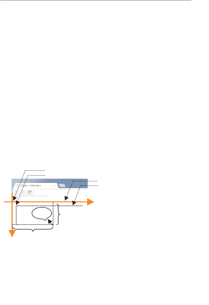
ptg11539634

CHAPTER 2 Your First Step with WebGL

56 x = ((x — rect.left) — canvas.height/2)/(canvas.height/2);

57 y = (canvas.width/2 — (y — rect.top))/(canvas.width/2);

58 // Store the coordinates to a_points array <- (1)

59 g_points.push(x); g_points.push(y);

61 // Clear <canvas>

62 gl.clear(gl.COLOR_BUFFER_BIT); <- (2)

64 var len = g_points.length;

65 for(var i = 0; i < len; i+=2) {

66 // Pass the position of a point to a_Position variable <- (3)

67 gl.vertexAttrib3f(a_Position, g_points[i], g_points[i+1], 0.0);

69 // Draw a point

70 gl.drawArrays(gl.POINTS, 0, 1);

71 }

72 }

The information about the position of a mouse click is stored as an event object and

passed by the browser using the argument

ev to the function click() . ev holds the posi-

tion information, and you can get the coordinates by using

ev.clientX and ev.clientY ,

as shown in lines 52 and 53. However, you cannot use the coordinates directly in this

sample program for two reasons:

1. The coordinate is the position in the “client area” in the browser, not in the

<canvas> (see Figure 2.26 ).

)0,0(

>savnac<foaeragniwardehT

>savnac<nigiroehT

Ytneilc.vednaXtneilc.ve

ehtninoitisopehtdloh

aeratneilc

resworbafoaeratneilcehT

Xtneilc.ve

Ytneilc.ve

aeratneilcfonigiroehT

!kcilC

Figure 2.26 The coordinate system of a browser’s client area and the position of the

2. The coordinate system of the

<canvas> is different from that of WebGL (see Figure

2.27 ) in terms of their origin and the direction of the y-axis.

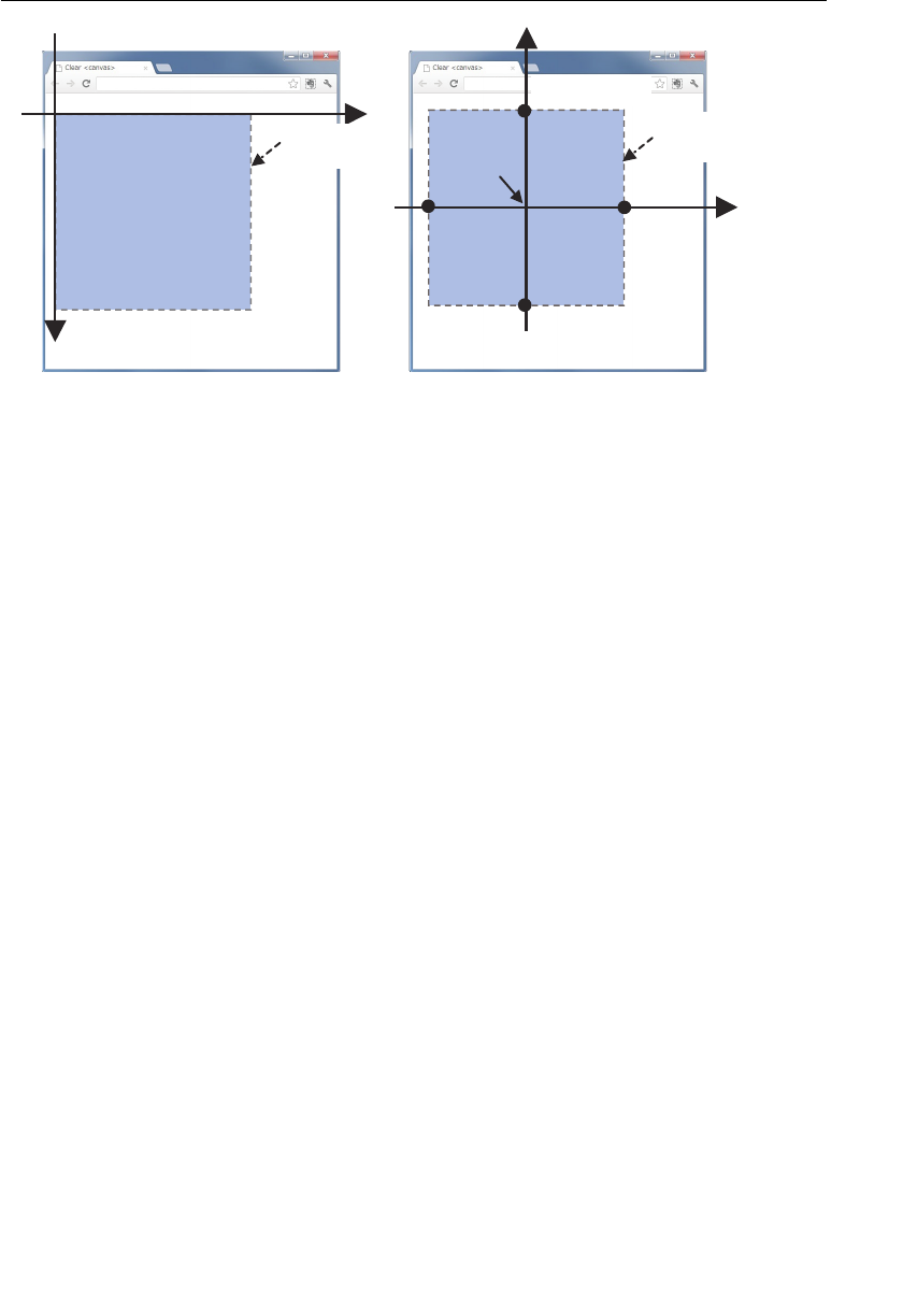
ptg11539634

Draw a Point with a Mouse Click 55

)0,0( y)0.0,0.1,0.

>savnac<

aeragniward

)0.0,0.0,0.1(

)0.0,0.0,0.1—(

)0.0,0.1—,0.0(

)0.0,0.0,0.0(

y)004,004(

>savnac<

aeragniward

Figure 2.27 The coordinate system of <canvas> (left) and that of WebGL on <canvas> (right)

First you need to transform the coordinates from the browser area to the canvas, and then

you need to transform them into coordinates that WebGL understands. Let’s look at how

to do that.

These transformations are performed at lines 56 and 57 in the sample program:

52 var x = ev.clientX;

53 var y = ev.clientY;

54 var rect = ev.target.getBoundingClientRect();

55 …

56 x = ((x — rect.left) — canvas.width/2)/(canvas.width/2);

57 y = (canvas.height/2 — (y — rect.top))/(canvas.height/2);

Line 54 gets the position of the <canvas> in the client area. The rect.left and rec.top

indicate the position of the origin of the

<canvas> in the browser’s client area (refer to

Figure 2.26 ). So,

(x – rect.left) at line 56 and (y – rect.top) at line 57 slide the posi-

tion (x, y) in the client area to the correct position on the

<canvas> element.

Next, you need to transform the <canvas> position into the WebGL coordinate system

shown in Figure 2.27 . To perform the transformation, you need to know the center posi-

tion of the

<canvas> . You can get the size of the <canvas> by canvas.height (in this case,

400) and

canvas.width (in this case, 400). So, the center of the element will be (canvas.

height/2, canvas.width/2) .

Next, you can implement this transformation by sliding the origin of the <canvas>

into the origin of the WebGL coordinate system located at the center of

<canvas> . The

((x — rect.left) — canvas.width/2) and (canvas.height/2 — (y -rect.top)) perform

the transformation.

Finally, as shown in Figure 2.27 , the range of the x-axis in the

<canvas> goes from 0 to

canvas.width (400), and that of the y-axis goes from 0 to canvas.height (400). Because

ptg11539634

CHAPTER 2 Your First Step with WebGL

the axes in WebGL range from –1.0 to 1.0, the last step is to map the range of the

<canvas> coordinate system to that of the WebGL coordinate system by dividing the x

coordinate by

canvas.width/2 and the y coordinate by canvas.height/2 . You can see this

division in lines 56 and 57.

Line 59 stores the resulting position of the mouse click in the array

g_points using the

push() method, which appends the data to the end of the array:

59 g_points.push(x); g_points.push(y);

So every time a mouse click occurs, the position of the click is appended to the array, as

shown in Figure 2.28 . (The length of the array is automatically stretched.) Note that the

index of an array starts from 0, so the first position is

g_points[0] .

xetanidrooc

ts1ehtfo

tniopdekcilc

yetanidrooc

ts1ehtfo

tniopdekcilc

xetanidrooc

dn2ehtfo

tniopdekcilc

yetanidrooc

dn2ehtfo

tniopdekcilc

x etanidrooc

dr3ehtfo

tniopdekcilc

yetanidrooc

dr3ehtfo

tniopdekcilc

…

][stniop_gfostnetnoceht

]2[stniop_g]1[stniop_g]0[stniop_g ]5[stniop_g]4[stniop_g]3[stniop_g

Figure 2.28 The content of g_points

You may be wondering why you need to store all the positions rather than just the most

recent mouse click. This is because of the way WebGL uses the color buffer. You will

remember from Figure 2.10 that in the WebGL system, first the drawing operation is

performed to the color buffer, and then the system displays its content to the screen. After

that, the color buffer is reinitialized and its content is lost. (This is the default behavior,

which you’ll investigate in the next section.) Therefore, it is necessary to save all the posi-

tions of the clicked points in the array, so that on each mouse click, the program can

draw all the previous points as well as the latest. For example, the first point is drawn at

the first mouse click. The first and second points are drawn at the second mouse click. The

first, second, and third points are drawn on the third click, and so on.

Returning to the program, the

<canvas> is cleared at line 62. After that, the for statement

at line 65 passes each position of the point stored in

g_points to a_Position in the vertex

shader. Then

gl.drawArrays() draws the point at that position:

65 for(var i = 0; i < len; i+=2) {

66 // Pass the position of a point to a_Position variable

67 gl.vertexAttrib3f(a_Position, g_points[i], g_points[i+1], 0.0);

Just like in HelloPoint2.js , you will use gl.vertexAttrib3f() to pass the point position

to the attribute variable

a_Position , which was passed as the fourth parameter of click()

at line 51.

ptg11539634

Draw a Point with a Mouse Click 57

The array g_points holds the x coordinate and y coordinate of the clicked points, as

shown in Figure 2.28 . Therefore,

g_points[i] holds the x coordinate, and g_points[i+1]

holds the y coordinate, so the loop index

i in the for statement at line 65 is incremented

by 2 using the convenient

+ operator.

Now that you have completed the preparations for drawing the point, the remaining task

is just to draw it using

gl.drawArrays() :

69 // Draw a point

70 gl.drawArrays(gl.POINTS, 0, 1);

Although it’s a little complicated, you can see that the use of event handlers combined

with attribute variable provides a flexible and generic means for user input to change what

WebGL draws.

Experimenting with the Sample Program

Now let’s experiment a little with this sample program ClickedPoints . After loading

ClickedPoints.html in your browser, every time you click, it draws a point at the clicked

position, as shown in Figure 2.26 .

Let’s examine what will happen when you stop clearing the

<canvas> at line 62.

Comment out the line as follows, and then reload the modified file into your browser.

61 // Clear <canvas>

62 // gl.clear(gl.COLOR_BUFFER_BIT);

64 var len = g_points.length;

65 for(var i = 0; i < len; i+=2) {

66 // Pass the position of a point to a_Position variable

67 gl.vertexAttrib3f(a_Position, g_points[i], g_points[i+1], 0.0);

69 // Draw a point

70 gl.drawArrays(gl.POINTS, 0, 1);

71 }

72 }

After running the program, you initially see a black background, but at the first click,

you see a red point on a white background. This is because WebGL reinitializes the color

buffer to the default value (0.0, 0.0, 0.0, 0.0) after drawing the point (refer to Table 2.1 ).

The alpha component of the default value is 0.0, which means the color is transparent.

Therefore, the color of the

<canvas> becomes transparent, so you see the background color

of the web page (white, in this case) through the

<canvas> element. If you don’t want this

behavior, you should use

gl.clearColor() to specify the clear color and then always call

gl.clear() before drawing something.

ptg11539634

CHAPTER 2 Your First Step with WebGL

Another interesting experiment is to look at how to simplify the code. In ClickedPoints.

js , the x and y coordinates are stored separately in the g_points array. However, you can

store the x and y coordinates as a group into the array as follows:

58 // Store the coordinates to a_points array <- (1)

59 g_points.push([x, y]);

In this case, the new two-element array [x, y] is stored as an element in the array

g_points . Conveniently, JavaScript can store an array in an array.

You can retrieve the x and y coordinates from the array as follows. First, you retrieve an

element from the array by specifying its index (line 66). Because the element itself is an

array containing (x, y), you can retrieve the first element and the second element as the

x and y coordinate of each point from the array (line 67):

65 for(var i = 0; i < len; i++) {

66 var xy = g_points[i];

67 gl.vertexAttrib3f(a_Position, xy[0], xy[1], 0.0);

…

71 }

In this way, you can deal with the x and y coordinates as a group, simplifying your

program and increasing the readability.

Change the Point Color

By now you should have a good feel for how the shaders work and how to pass data to

them from your JavaScript program. Let’s build on your understanding by constructing a

more complex program that draws points whose colors vary depending on their position

on the

<canvas> .

You already studied how to change the color of a point when you looked at HelloPoint1 .

In that example, you modified the fragment shader program directly to embed the color

value into the shader. In this section, let’s construct the program so that you can specify

the color of a point from JavaScript. This is similar to

HelloPoint2 earlier, where you

passed the position of a point from a JavaScript program to the vertex shader. However,

in this sample program, you need to pass the data to a “fragment shader,” not to a vertex

shader.

The name of the sample program is

ColoredPoints . If you load the example into your

browser, the result is the same as

ClickedPoints except that each point’s color varies

depending on its position (see Figure 2.29 ).

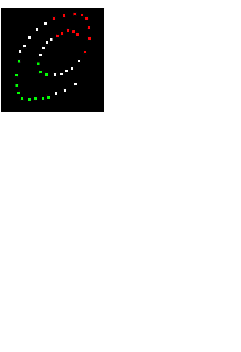
ptg11539634

Change the Point Color 59

Figure 2.29 ColoredPoints

To pass data to a fragment shader, you can use a uniform variable and follow the same

steps that you used when working with attribute variables. However, this time the target is

a fragment shader, not a vertex shader:

1. Prepare the uniform variable for the color in the fragment shader.

2. Assign the uniform variable to the

gl_FragColor variable.

3. Pass the color data to the uniform variable from the JavaScript program.

Let’s look at the sample program and see how these steps are programmed.

Sample Program (ColoredPoints.js)

The vertex shader of this sample program is the same as in ClickedPoints.js . However,

this time, the fragment shader plays a more important role because the program changes

the color of the point dynamically and, as you will remember, fragment shaders handle

colors. Listing 2.8 shows

ColoredPoints.js .

Listing 2.8 ColoredPoints.js

1 // ColoredPoints.js

2 // Vertex shader program

3 var VSHADER_SOURCE =

4 ‘attribute vec4 a_Position;n’ +

5 ‘void main() {n’ +

6 ‘ gl_Position = a_Position;n’ +

7 ‘ gl_PointSize = 10.0;n’ +

ptg11539634

CHAPTER 2 Your First Step with WebGL

8 ‘}n’;

10 // Fragment shader program

11 var FSHADER_SOURCE =

12 ‘precision mediump float;n’ +

13 ‘uniform vec4 u_FragColor;n’ + // uniform variable <- (1)

14 ‘void main() {n’ +

15 ‘ gl_FragColor = u_FragColor;n’ + <- (2)

16 ‘}n’;

18 function main() {

…

29 // Initialize shaders

30 if (!initShaders(gl, VSHADER_SOURCE, FSHADER_SOURCE)) {

…

33 }

35 // Get the storage location of a_Position variable

36 var a_Position = gl.getAttribLocation(gl.program, ‘a_Position’);

…

42 // Get the storage location of u_FragColor variable

43 var u_FragColor = gl.getUniformLocation(gl.program, ‘u_FragColor’);

…

49 // Register function (event handler) to be called on a mouse press

50 canvas.onmousedown = function(ev){ click(ev, gl, canvas, a_Position,

➥u_FragColor) };

…

56 gl.clear(gl.COLOR_BUFFER_BIT);

57 }

59 var g_points = []; // The array for a mouse press

60 var g_colors = []; // The array to store the color of a point

61 function click(ev, gl, canvas, a_Position, u_FragColor) {

62 var x = ev.clientX; // x coordinate of a mouse pointer

63 var y = ev.clientY; // y coordinate of a mouse pointer

64 var rect = ev.target.getBoundingClientRect();

66 x = ((x — rect.left) — canvas.width/2)/(canvas.width/2);

67 y = (canvas.height/2 — (y — rect.top))/(canvas.height/2);

69 // Store the coordinates to g_points array

70 g_points.push([x, y]);

71 // Store the color to g_colors array

72 if(x >= 0.0 && y >= 0.0) { // First quadrant

73 g_colors.push([1.0, 0.0, 0.0, 1.0]); // Red

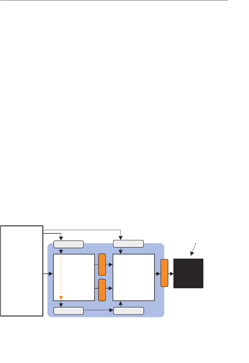
ptg11539634

Change the Point Color 61

74 } else if(x < 0.0 && y < 0.0) { // Third quadrant

75 g_colors.push([0.0, 1.0, 0.0, 1.0]); // Green

76 } else { // Others

77 g_colors.push([1.0, 1.0, 1.0, 1.0]); // White

78 }

80 // Clear <canvas>

81 gl.clear(gl.COLOR_BUFFER_BIT);

83 var len = g_points.length;

84 for(var i = 0; i < len; i++) {

85 var xy = g_points[i];

86 var rgba = g_colors[i];

88 // Pass the position of a point to a_Position variable

89 gl.vertexAttrib3f(a_Position, xy[0], xy[1], 0.0);

90 // Pass the color of a point to u_FragColor variable

91 gl.uniform4f(u_FragColor, rgba[0],rgba[1],rgba[2],rgba[3]); <-(3)

92 // Draw a point

93 gl.drawArrays(gl.POINTS, 0, 1);

94 }

95 }

Uniform Variables

You likely remember how to use an attribute variable to pass data from a JavaScript

program to a vertex shader. Unfortunately, the attribute variable is only available in a

vertex shader, and when using a fragment shader, you need to use a uniform variable.

There is an alternative mechanism, a varying variable (bottom of Figure 2.30 ); however,

it is more complex, so you won’t use it until Chapter 5 .

redahSxetreV tnemgarF

redahS

gl_Positiongl_PointSize

gl_FragColor

elbairavetubirtta elbairavmrofinu

tpircSavaJ

{)(niamnoitcnuf

…LGbeWteg=lgrav

…

;)…(sredahStini

…

}

elbairavgniyrav

reffuBroloC

elbairavgniyrav

Figure 2.30 Two ways of passing a data to a fragment shader

ptg11539634

CHAPTER 2 Your First Step with WebGL

When you were introduced to attribute variables, you saw that a uniform variable is a

variable for passing “uniform” (nonvariable) data from a JavaScript program to all vertices

or fragments in the shader. Let’s now use that property.

Before using a uniform variable, you need to declare the variable using the form

<Storage

Qualifier> <Type> <Variable name> in the same way (see Figure 2.31 ) as declaring an

attribute variable. (See the section “Sample Program (HelloPoint2.js).”)

roloC

arF

u4cevmrofinu

emaNelbairaVepyTreifilauQegarotS

Figure 2.31 The declaration of the uniform variable

In this sample program, the uniform variable

u_FragColor is named after the variable

gl_FragColor because you will assign the uniform variable to the gl_FragColor later.

The

u_ in u_FragColor is part of our programming convention and indicates that it is a

uniform variable. You need to specify the same data type as

gl_FragColor for u_FragColor

because you can only assign the same type of variable to

gl_FragColor . Therefore, you

prepare

u_FragColor at line 13, as follows:

10 // Fragment shader program

11 var FSHADER_SOURCE =

12 ‘precision mediump float;n’ +

13 ‘uniform vec4 u_FragColor;n’ + // uniform variable

14 ‘void main() {n’ +

15 ‘ gl_FragColor = u_FragColor;n’ +

16 ‘}n’;

Note that line 12 specifies the range and precision of variables by using a precision quali-

fier , in this case medium precision, which is covered in detail in Chapter 5 .

Line 15 assigns the color in the uniform variable

u_FragColor to gl_FragColor , which

causes the point to be drawn in whatever color is passed. Passing the color through the

uniform variable is similar to using an attribute variable; you need to retrieve the storage

location of the variable and then write the data to the location within the JavaScript

program.

Retrieving the Storage Location of a Uniform Variable

You can use the following method to retrieve the storage location of a uniform variable.

5 In GLSL ES, you can only specify float data types for an attribute variable; however, you can

specify any type for a uniform variable. (See Chapter 6 for more details.)

ptg11539634

Change the Point Color 63

gl.getUniformLocation(program, name)

Retrieve the storage location of the uniform variable specified by the name parameter.

Parameters program Specifies the program object that holds a vertex

shader and a fragment shader.

name Specifies the name of the uniform variable whose loca-

tion is to be retrieved.

Return value non-null The location of the specified uniform variable.

null The specified uniform variable does not exist or its

name starts with the reserved prefix

gl_ or webgl_ .

Errors INVALID_OPERATION program has not been successfully linked

(See Chapter 9 .)

INVALID_VALUE The length of name is more than the maximum length

(256 by default) of a uniform variable.

The functionality and parameters of this method are the same as in

gl.getAttribLoca-

tion() . However, the return value of this method is null , not –1, if the uniform variable

does not exist or its name starts with a reserved prefix. For this reason, unlike attribute

variables, you need to check whether the return value is

null . You can see this error

checking line 44. In JavaScript,

null can be treated as false when checking the condition

of an

if statement, so you can use the ! operator to check the result:

42 // Get the storage location of uniform variable

43 var u_FragColor = gl.getUniformLocation(gl.program, ‘u_FragColor’);

44 if (!u_FragColor) {

45 console.log(‘Failed to get u_FragColor variable’);

46 return;

47 }

Assigning a Value to a Uniform Variable

Once you have the location of the uniform variable and the WebGL method, gl.

uniform4f() is used to write data to it. It has the same functionality and parameters as

those of

gl.vertexAttrib[1234]f() .

ptg11539634

CHAPTER 2 Your First Step with WebGL

gl.uniform4f (location, v0, v1, v2, v3)

Assign the data specified by v0 , v1 , v2 , and v3 to the uniform variable specified by

location .

Parameters location Specifies the storage location of a uniform variable to

be modified.

v0 Specifies the value to be used as the first element of

the uniform variable.

v1 Specifies the value to be used as the second element

of the uniform variable.

v2 Specifies the value to be used as the third element of

the uniform variable.

v3 Specifies the value to be used as the fourth element of

the uniform variable.

Return value None

Errors INVALID_OPERATION There is no current program object.

location is an invalid uniform variable location.

Let’s look at the portion of the sample program where the

gl.uniform4f() method is used

to assign the data (line 91). As you can see, several processing steps are needed in advance:

71 // Store the color to g_colors array

72 if(x >= 0.0 && y >= 0.0) { // First quadrant

73 g_colors.push([1.0, 0.0, 0.0, 1.0]); // Red

74 } else if(x < 0.0 && y < 0.0) { // Third quadrant

75 g_colors.push([0.0, 1.0, 0.0, 1.0]); // Green

76 } else { // Other quadrants

77 g_colors.push([1.0, 1.0, 1.0, 1.0]); // White

78 }

…

83 var len = g_points.length;

84 for(var i = 0; i < len; i++) {

85 var xy = g_points[i];

86 var rgba = g_colors[i];

…

91 gl.uniform4f(u_FragColor, rgba[0], rgba[1], rgba[2], rgba[3]);

To understand this program logic, let’s return to the goal of this program, which is to vary

the color of a point according to where on the

<canvas> the mouse is clicked. In the first

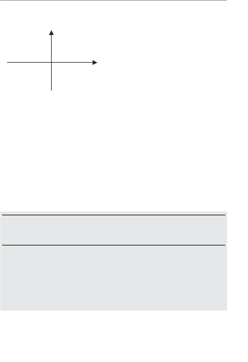
ptg11539634

Change the Point Color 65

quadrant, the color is set to red; in the third quadrant, the color is green; in the other

quadrants, the color is white (see Figure 2.32 ).

tnardauqdnoceS

)etihw(

tnardauqtsriF

)der(

tnardauqdrihT

)neerg(

tnardauqhtruoF

)etihw(

Figure 2.32 The name of each quadrant in a coordinate system and its drawing colors

The code from lines 72 to 78 simply determines which quadrant the mouse click was in

and then, based on that, writes the appropriate color into the array

g_colors . Finally, at

line 84, the program loops through the points, passing the correct color to the uniform

variable

u_FragColor at line 91. This causes WebGL to write all the points stored so far to

the color buffer, which then results in the browser display being updated.

Before finishing this chapter, let’s take a quick look at the rest of the family methods for

gl.uniform[1234]f() .

Family Methods of gl.uniform4f()

gl.uniform4f() also has a family of methods. gl.uniform1f() is a method to assign a

single value (v0),

gl.uniform2f() assigns two values (v0 and v1), and gl.uniform3f()

assigns three values (v0, v1, and v2).

gl.uniform1f(location, v0)

gl.uniform2f(location, v0, v1)

gl.uniform3f(location, v0, v1, v2)

gl.uniform4f(location, v0, v1, v2, v3)

Assign data to the uniform variable specified by location .

gl.uniform1f() indicates

that only one value is passed, and it will be used to modify the first component of

the uniform variable. The second and third components will be set to 0.0, and the

fourth component will be set to 1.0. Similarly,

gl.uniform2f() indicates that values are

provided for the first two components, the third component will be set to 0.0, and the

fourth component will be set to 1.0.

gl.uniform3f() indicates that values are provided

for the first three components and the fourth component will be set to 1.0, whereas

gl.unifrom4f() indicates that values are provided for all four components.

ptg11539634

CHAPTER 2 Your First Step with WebGL

Parameters location Specifies the storage location of a uniform variable.

v0, v1, v2, v3 Specifies the values to be assigned to the first,

second, third, and fourth component of the uniform

variable.

Return value None

Errors INVALID_OPERATION There is no current program object.

location is an invalid uniform variable location.

Summary

In this chapter, you saw the core functions of WebGL and how to use them. In particu-

lar, you learned about shaders, which are the main mechanism used in WebGL to draw

graphics. Based on this, you constructed several sample programs starting with a simple

program to draw a red point, and then you added complexity by changing its position

based on a mouse click and changed its color. In both cases, these examples helped you

understand how to pass data from a JavaScript program to the shaders, which will be criti-

cal for future examples.

The shapes found in this chapter were still just two-dimensional points. However, you can

apply the same knowledge of the use of the core WebGL functions and shaders to more

complex shapes and to three-dimensional objects.

A key learning point in this chapter is this: A vertex shader performs per-vertex opera-

tions, and a fragment shader performs per-fragment operations. The following chapters

explain some of the other functions of WebGL, while slowly increasing the complexity of

the shapes that you manipulate and display on the screen.

ptg11539634

Chapter 3

Drawing and Transforming Triangles

Chapter 2 , “Your First Step with WebGL,” explained the basic approach to drawing WebGL

graphics. You saw how to retrieve the WebGL context and clear a

<canvas> in preparation for

drawing your 2D/3DCG. You then explored the roles and features of the vertex and fragment

shaders and how to actually draw graphics with them. With this basic structure in mind, you

then constructed several sample programs that drew simple shapes composed of points on the

screen.

This chapter builds on those basics by exploring how to draw more complex shapes and how to

manipulate those shapes in 3D space. In particular, this chapter looks at

• The critical role of triangles in 3DCG and WebGL’s support for drawing triangles

• Using multiple triangles to draw other basic shapes

• Basic transformations that move, rotate, and scale triangles using simple equations

• How matrix operations make transformations simple

By the end of this chapter, you will have a comprehensive understanding of WebGL’s support for

drawing basic shapes and how to use matrix operations to manipulate those shapes. Chapter 4 ,

“More Transformations and Basic Animation,” then builds on this knowledge to explore simple

animations.

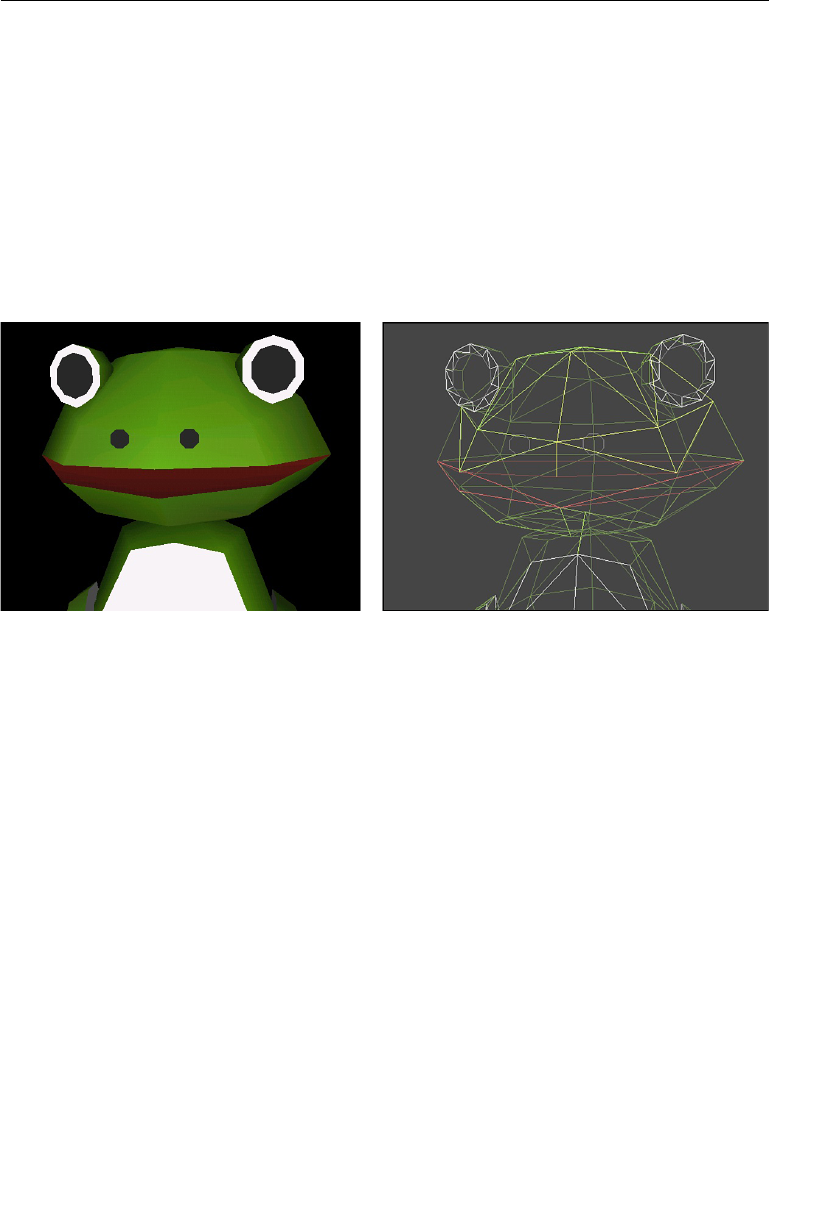
ptg11539634

CHAPTER 3 Drawing and Transforming Triangles

Drawing Multiple Points

As you are probably aware , 3D models are actually made from a simple building block:

the humble triangle. For example, looking at the frog in Figure 3.1 , the figure on the right

side shows the triangles used to make up the shape, and in particular the three vertices

that make up one triangle of the head. So, although this game character has a complex

shape, its basic components are the same as a simple one, except of course for many more

triangles and their associated vertices. By using smaller and smaller triangles, and there-

fore more and more vertices, you can create more complex or smoother objects. Typically,

a complex shape or game character will consist of tens of thousands of triangles and

their associated vertices. Thus, multiple vertices used to make up triangles are pivotal for

drawing 3D objects.

Figure 3.1 Complex characters are also constructed from multiple triangles

In this section, you explore the process of drawing shapes using multiple vertices.

However, to keep things simple, you’ll continue to use 2D shapes, because the technique

to deal with multiple vertices for a 2D shape is the same as dealing with them for a 3D

object. Essentially, if you can master these techniques for 2D shapes, you can easily under-

stand the examples in the rest of this book that use the same techniques for 3D objects.

As an example of handling multiple vertices, let’s create a program,

MultiPoint , that

draws three red points on the screen; remember, three points or vertices make up the

triangle. Figure 3.2 shows a screenshot from

Multipoint .

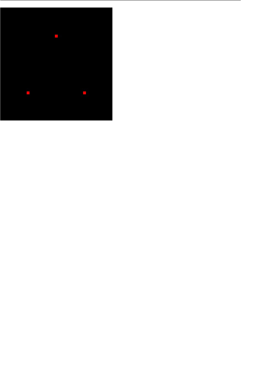
ptg11539634

Drawing Multiple Points 69

Figure 3.2 MultiPoint

In the previous chapter, you created a sample program,

ClickedPoints , that drew multi-

ple points based on mouse clicks.

ClickedPoints stored the position of the points in a

JavaScript array (

g_points[] ) and used the gl.drawArrays() method to draw each point

( Listing 3.1 ). To draw multiple points, you used a loop that iterated through the array,

drawing each point in turn by passing one vertex at a time to the shader.

Listing 3.1 Drawing Multiple Points as Shown in ClickedPoints.js ( Chapter 2 )

65 for(var i = 0; i<len; i+=2) {

66 // Pass the position of a point to a_Position variable

67 gl.vertexAttrib3f(a_Position, g_points[i], g_points[i+1], 0.0);

69 // Draw a point

70 gl.drawArrays(gl.POINTS, 0, 1);

71 }

Obviously, this method is useful only for single points. For shapes that use multiple verti-

ces, you need a way to simultaneously pass multiple vertices to the vertex shader so that

you can draw shapes constructed from multiple vertices, such as triangles, rectangles, and

cubes.

WebGL provides a convenient way to pass multiple vertices and uses something called a

buffer object to do so. A buffer object is a memory area that can store multiple vertices in

the WebGL system. It is used both as a staging area for the vertex data and a way to simul-

taneously pass the vertices to a vertex shader.

Let’s examine a sample program before explaining the buffer object so you can get a feel

for the processing flow.

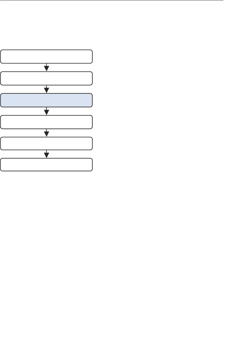
ptg11539634

CHAPTER 3 Drawing and Transforming Triangles

Sample Program (MultiPoint.js)

The processing flowchart for MultiPoint.js (see Figure 3.3 ) is basically the same as for

ClickedPoints.js ( Listing 2.7 ) and ColoredPoints.js ( Listing 2.8 ), which you saw in

Chapter 2 . The only difference is a new step, setting up the positions of vertices, which is

added to the previous flow.

LGbeWroftxetnocgnirednerehtteG

>savnac<raelC

sredahsezilaitinI

warD

>savnac<gniraelcrofrolocehtteS

secitrevfosnoitisopehtteS

Figure 3.3 Processing flowchart for MultiPoints.js

This step is implemented at line 34, the function

initVertexBuffers() , in Listing 3.2 .

Listing 3.2 MultiPoint. js

1 // MultiPoint.js

2 // Vertex shader program

3 var VSHADER_SOURCE =

4 ‘attribute vec4 a_Position;n’ +

5 ‘void main() {n’ +

6 ‘ gl_Position = a_Position;n’ +

7 ‘ gl_PointSize = 10.0;n’ +

8 ‘}n’;

10 // Fragment shader program

…

16 function main() {

…

ptg11539634

Drawing Multiple Points 71

20 // Get the rendering context for WebGL

21 var gl = getWebGLContext(canvas);

…

27 // Initialize shaders

28 if (!initShaders(gl, VSHADER_SOURCE, FSHADER_SOURCE)) {

…

31 }

33 // Set the positions of vertices

34 var n = initVertexBuffers(gl);

35 if (n < 0) {

36 console.log(‘Failed to set the positions of the vertices’);

37 return;

38 }

40 // Set the color for clearing <canvas>

…

43 // Clear <canvas>

…

46 // Draw three points

47 gl.drawArrays(gl.POINTS, 0, n); // n is 3

48 }

50 function initVertexBuffers(gl) {

51 var vertices = new Float32Array([

52 0.0, 0.5, -0.5, -0.5, 0.5, -0.5

53 ]);

54 var n = 3; // The number of vertices

56 // Create a buffer object

57 var vertexBuffer = gl.createBuffer();

58 if (!vertexBuffer) {

59 console.log(‘Failed to create the buffer object ‘);

60 return -1;

61 }

63 // Bind the buffer object to target

64 gl.bindBuffer(gl.ARRAY_BUFFER, vertexBuffer);

65 // Write date into the buffer object

66 gl.bufferData(gl.ARRAY_BUFFER, vertices, gl.STATIC_DRAW);

68 var a_Position = gl.getAttribLocation(gl.program, ‘a_Position’);

…

73 // Assign the buffer object to a_Position variable

74 gl.vertexAttribPointer(a_Position, 2, gl.FLOAT, false, 0, 0);

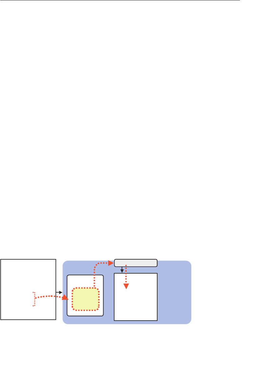
ptg11539634

CHAPTER 3 Drawing and Transforming Triangles

76 // Enable the assignment to a_Position variable

77 gl.enableVertexAttribArray(a_Position);

79 return n;

80 }

The new function initVertexBuffers() is defined at line 50 and used at line 34 to set

up the vertex buffer object. The function stores multiple vertices in the buffer object and

then completes the preparations for passing it to a vertex shader:

33 // Set the positions of vertices

34 var n = initVertexBuffers(gl);

The return value of this function is the number of vertices being drawn, stored in the vari-

able

n . Note that in case of error, n is negative.

As in the previous examples, the drawing operation is carried out using a single call to

gl.drawArrays() at Line 48. This is similar to ClickedPoints.js except that n is passed as

the third argument of

gl.drawArrays() rather than the value 1:

46 // Draw three points

47 gl.drawArrays(gl.POINTS, 0, n); // n is 3

Because you are using a buffer object to pass multiple vertices to a vertex shader in init-

VertexBuffers() , you need to specify the number of vertices in the object as the third

parameter of

gl.drawArrays() so that WebGL then knows to draw a shape using all the

vertices in the buffer object.

Using Buffer Objects

As indicated earlier, a buffer object is a mechanism provided by the WebGL system that

provides a memory area allocated in the system (see Figure 3.4 ) that holds the vertices you

want to draw. By creating a buffer object and then writing the vertices to the object, you

can pass multiple vertices to a vertex shader through one of its attribute variables.

redahSxetreV

attribute variable

{)(niamnoitcnuf

=secitrevrav

[(yarrA23taolFwen

,5.0,0.0

,5.0—,5.0—

5.0—,5.0

;)]

;),secitrev,..(atareffub.lg

LGbeW

metsyS

,5.0,0.0

,5.0—,5.0—

5.0—,5.0

tcejbOreffuB

5 . 0 , 0 . 0

5 . 0 — , 5 . 0 —

5 . 0 — , 5 . 0

tpircSavaJ

Figure 3.4 Passing multiple vertices to a vertex shader by using a buffer object

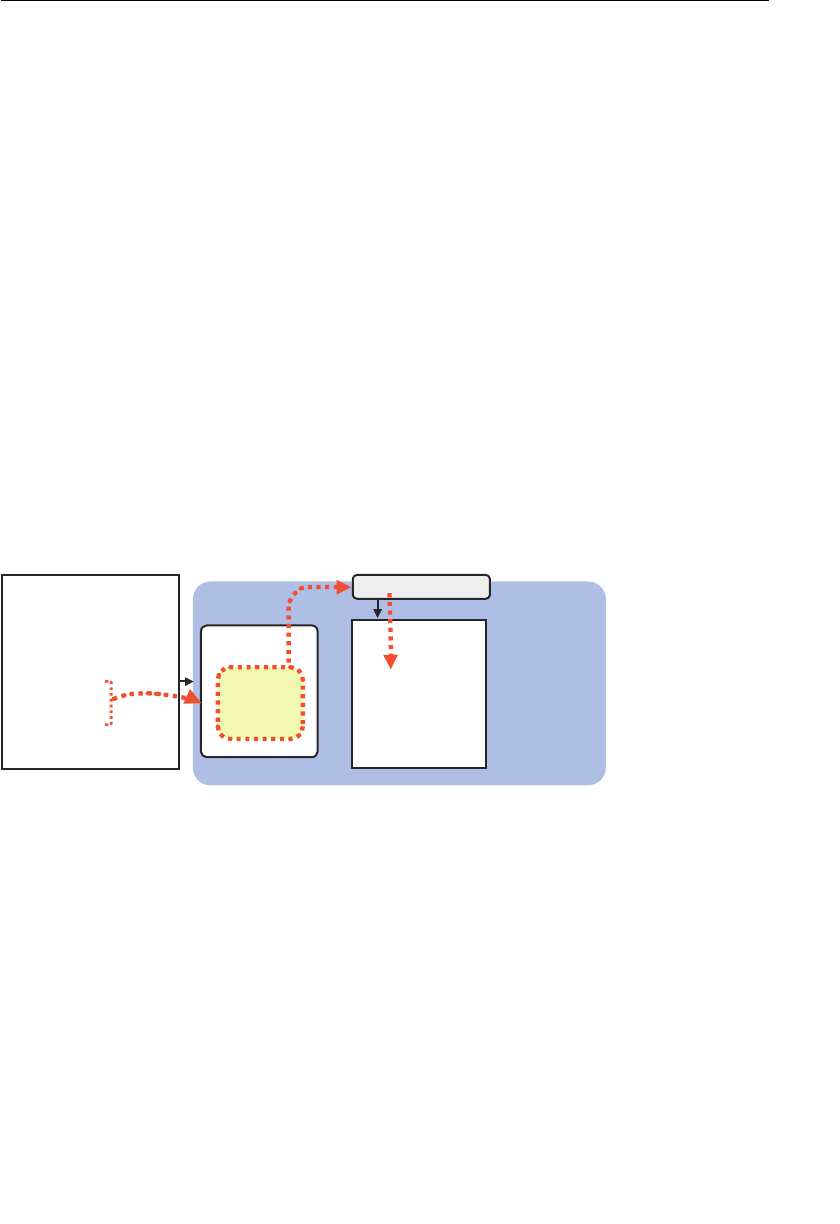
ptg11539634

Drawing Multiple Points 73

In the sample program, the data (vertex coordinates) written into a buffer object is defined

as a special JavaScript array (

Float32Array ) as follows. We will explain this special array in

detail later, but for now you can think of it as a normal array:

51 var vertices = new Float32Array([

52 0.0, 0.5, -0.5, -0.5, 0.5, -0.5

53 ]);

There are five steps needed to pass multiple data values to a vertex shader through a buffer

object. Because WebGL uses a similar approach when dealing with other objects such as

texture objects ( Chapter 4 ) and framebuffer objects ( Chapter 8 , “Lighting Objects”), let’s

explore these in detail so you will be able to apply the knowledge later:

1. Create a buffer object (

gl.createBuffer() ).

2. Bind the buffer object to a target (

gl.bindBuffer() ).

3. Write data into the buffer object ( gl.bufferData() ).

4. Assign the buffer object to an attribute variable ( gl.vertexAttribPointer() ).

5. Enable assignment ( gl.enableVertexAttribArray() ).

Figure 3.5 illustrates the five steps.

{)(niamnoitcnuf

=secitrevrav

[(yarrA23taolFwen

,5.0,0.0

,5.0—,5.0—

5.0—,5.0

;)]

;),secitrev,..(atareffub.lg

,5.0,0.0

,5.0—,5.0—

5.0—,5.0

tcejbOreffuB

5.0,0.0

5.0—,5.0—

5.0—,5.0

(1)(2)

(4) (5)

redahSxetreV

tpircSavaJ

LGbeW

metsyS

(3)

attribute variable

Figure 3.5 The five steps to pass multiple data values to a vertex shader using a buffer object

The code performing the steps in the sample program in Listing 3.2 is as follows:

56 // Create a buffer object <- (1)

57 var vertexBuffer = gl.createBuffer();

58 if (!vertexBuffer) {

59 console.log(‘Failed to create a buffer object’);

60 return -1;

61 }

63 // Bind the buffer object to a target <- (2)

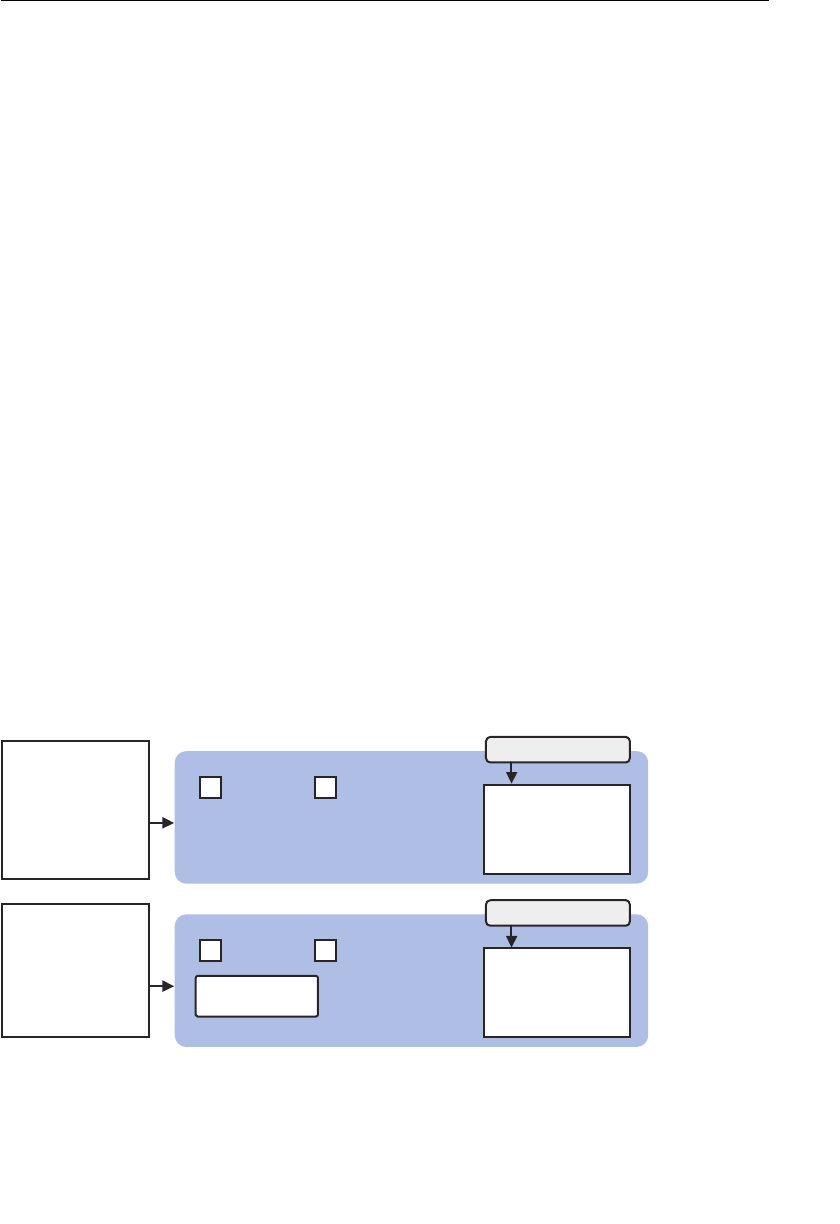
ptg11539634

CHAPTER 3 Drawing and Transforming Triangles

64 gl.bindBuffer(gl.ARRAY_BUFFER, vertexBuffer);

65 // Write date into the buffer object <- (3)

66 gl.bufferData(gl.ARRAY_BUFFER, vertices, gl.STATIC_DRAW);

68 var a_Position = gl.getAttribLocation(gl.program, ‘a_Position’);

…

73 // Assign the buffer object to a_Position variable <- (4)

74 gl.vertexAttribPointer(a_Position, 2, gl.FLOAT, false, 0, 0);

76 // Enable the assignment to a_Position variable <- (5)

77 gl.enableVertexAttribArray(a_Position);

Let’s start with the first three steps (1–3), from creating a buffer object to writing data

(vertex coordinates in this example) to the buffer, explaining the methods used within

each step.

Create a Buffer Object (gl.createBuffer())

Before you can use a buffer object, you obviously need to create the buffer object. This is

the first step, and it’s carried out at line 57:

57 var vertexBuffer = gl.createBuffer();

You use the gl.createBuffer() method to create a buffer object within the WebGL

system. Figure 3.6 shows the internal state of the WebGL system. The upper part of the

figure shows the state before executing the method, and the lower part is after execution.

As you can see, when the method is executed, it results in a single buffer object being

created in the WebGL system. The keywords

gl.ARRAY_BUFFER and gl.ELEMENT_ARRAY_

BUFFER in the figure will be explained in the next section, so you can ignore them for

now.

redahSxetreV

tcejbOreffuB

REFFUB_YARRA.lg

{)(niamnoitcnuf

…LGbeWteg=lgrav

…

;)…(reffuBetaerc.lg

redahSxetreV

REFFUB_YARRA.lg

{)(niamnoitcnuf

…LGbeWteg=lgrav

…

REFFUB_YARRA_TNEMELE.lg

tpircSavaJ

attribute variable

Figure 3.6 Create a buffer object

ptg11539634

Drawing Multiple Points 75

The following shows the specification of gl.createBuffer() .

gl.createBuffer ()

Create a buffer object.

Return value non-null The newly created buffer object.

null Failed to create a buffer object.

Errors None

The corresponding method

gl.deleteBuffer() deletes the buffer object created by

gl.createBuffer() .

gl.deleteBuffer (buffer)

Delete the buffer object specified by buffer.

Parameters buffer Specifies the buffer object to be deleted.

Return Value None

Errors None

Bind a Buffer Object to a Target (gl.bindBuffer())

After creating a buffer object, the second step is to bind it to a “target.” The target tells

WebGL what type of data the buffer object contains, allowing it to deal with the contents

correctly. This binding process is carried out at line 64 as follows:

64 gl.bindBuffer(gl.ARRAY_BUFFER, vertexBuffer);

The specification of gl.bindBuffer() is as follows.

gl.bindBuffer(target, buffer)

Enable the buffer object specified by buffer and bind it to the target.

Parameters Target can be one of the following:

gl.ARRAY_BUFFER Specifies that the buffer object contains vertex data.

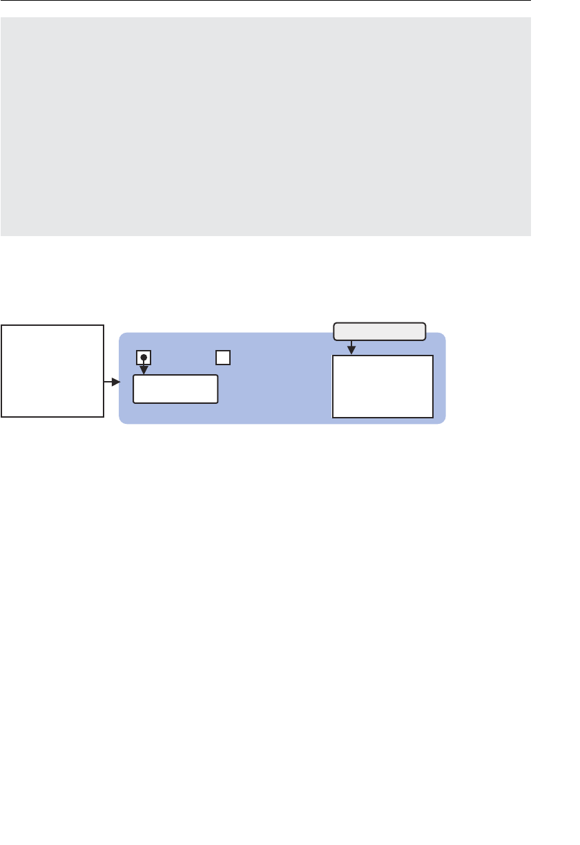
ptg11539634

CHAPTER 3 Drawing and Transforming Triangles

gl.ELEMENT_

ARRAY_BUFFER

Specifies that the buffer object contains index values

pointing to vertex data. (See Chapter 6 , “The OpenGL

ES Shading Language [GLSL ES].)

buffer Specifies the buffer object created by a previous call to

gl.createBuffer() .

When

null is specified, binding to the target is

disabled.

Return Value None

Errors INVALID_ENUM target is none of the above values. In this case, the

current binding is maintained.

In the sample program in this section,

gl.ARRAY_BUFFER is specified as the target to store

vertex data (positions) in the buffer object. After executing line 64, the internal state in

the WebGL system changes, as shown in Figure 3.7 .

redahSxetreV

tcejbOreffuB

REFFUB_YARRA.lg

tpircSavaJ

{)(niamnoitcnuf

…LGbeWteg=lgrav

…

;)…(reffuBdnib.lg

REF

FUB_YARRA_TNEMELE.l

attribute variable

Figure 3.7 Bind a buffer object to a target

The next step is to write data into the buffer object. Note that because you won’t be using

the

gl.ELEMENT_ARRAY_BUFFER until Chapter 6 , it’ll be removed from the following figures

for clarity.

Write Data into a Buffer Object (gl.bufferData())

Step 3 allocates storage and writes data to the buffer. You use gl.bufferData() to do this,

as shown at line 66:

66 gl.bufferData(gl.ARRAY_BUFFER, vertices, gl.STATIC_DRAW);

This method writes the data specified by the second parameter ( vertices ) into the buffer

object bound to the first parameter (

gl.ARRAY_BUFFER ). After executing line 66, the inter-

nal state of the WebGL system changes, as shown in Figure 3.8 .

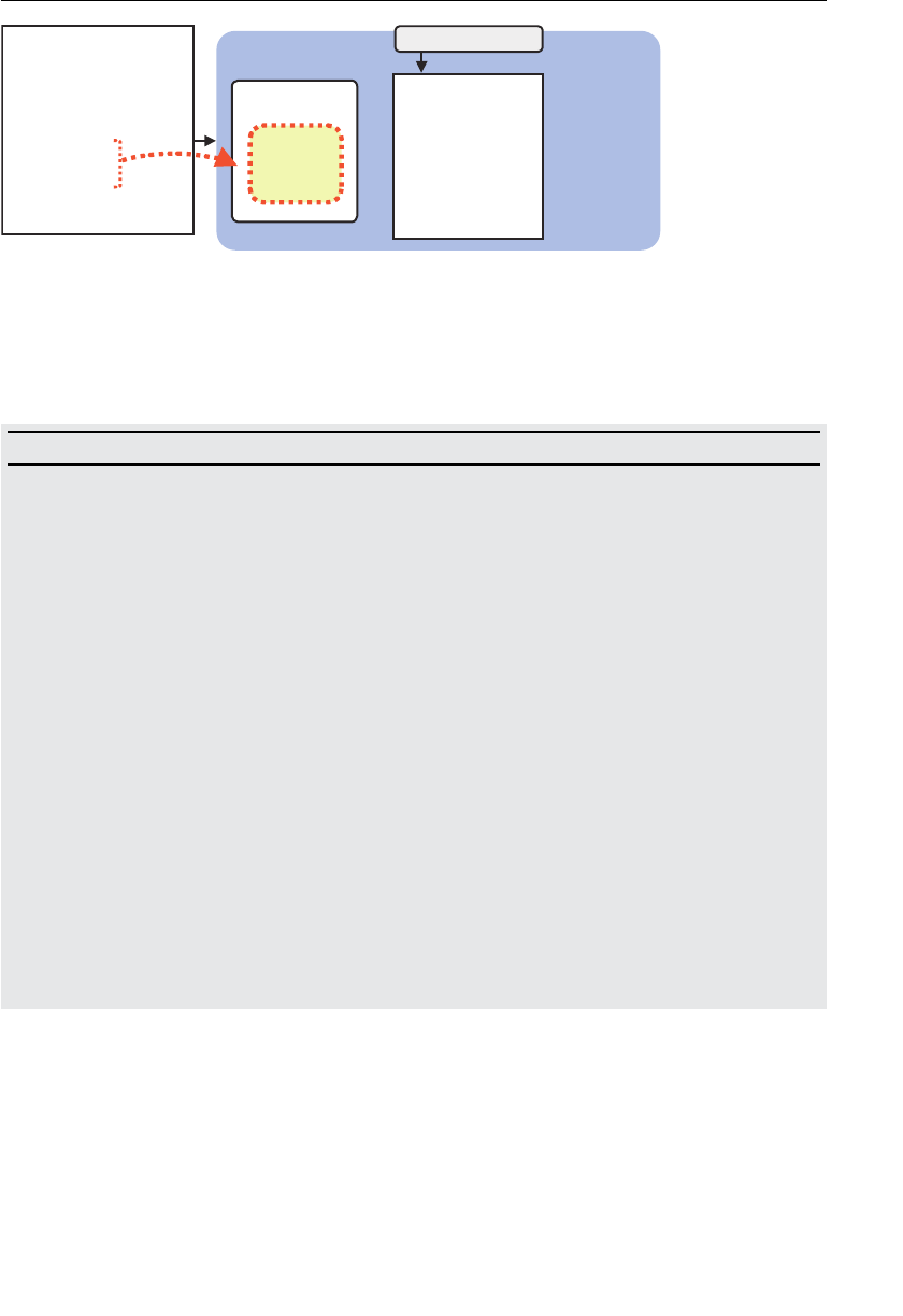
ptg11539634

Drawing Multiple Points 77

redahSxetreV

{)(niamnoitcnuf

=secitrevrav

[(yarrA23taolFwen

,5.0,0.0

,5.0—,5.0—

5.0—,5.0

;)]

;),secitrev,..(

tcejbOreffuB

5.0,0.0

5.0—,5.0—

5.0—,5.0

.at

reffublg D

tpircSavaJ

LGbeW

metsyS

attribute variable

Figure 3.8 Allocate storage and write data into a buffer object

You can see in this figure that the vertex data defined in your JavaScript program is

written to the buffer object bound to gl.ARRAY_BUFFER . The following table shows the

specification of

gl.bufferData() .

gl.bufferData(target, data, usage)

Allocate storage and write the data specified by data to the buffer object bound to target.

Parameters target Specifies

gl.ARRAY_BUFFER or gl.ELEMENT_ARRAY_BUFFER.

data Specifies the data to be written to the buffer object (typed

array; see the next section).

usage Specifies a hint about how the program is going to use

the data stored in the buffer object. This hint helps WebGL

optimize performance but will not stop your program from

working if you get it wrong.

gl.STATIC_

DRAW

The buffer object data will be specified once

and used many times to draw shapes.

gl.STREAM_

DRAW

The buffer object data will be specified once

and used a few times to draw shapes.

gl.DYNAMIC_

DRAW

The buffer object data will be specified repeat-

edly and used many times to draw shapes.

Return value None

Errors INVALID_ENUM target is none of the preceding constants

Now, let us examine what data is passed to the buffer object using

gl.bufferData() .

This method uses the special array

vertices mentioned earlier to pass data to the vertex

shader. The array is created at line 51 using the

new operator with the data arranged as

<x coordinate and y coordinate of the first vertex>, <x coordinate and y coordinate of the

second vertex>, and so on:

ptg11539634

CHAPTER 3 Drawing and Transforming Triangles

51 var vertices = new Float32Array([

52 0.0, 0.5, -0.5, -0.5, 0.5, -0.5

53 ]);

54 var n = 3; // The number of vertices

As you can see in the preceding code snippet, you are using the Float32Array object

instead of the more usual JavaScript Array object to store the data. This is because the

standard array in JavaScript is a general-purpose data structure able to hold both numeric

data and strings but isn’t optimized for large quantities of data of the same type, such as

vertices . To address this issue, the typed array, of which one example is Float32Array ,

has been introduced.

Typed Arrays

WebGL often deals with large quantities of data of the same type, such as vertex coordi-

nates and colors, for drawing 3D objects. For optimization purposes, a special type of array

( typed array ) has been introduced for each data type. Because the type of data in the

array is known in advance, it can be handled efficiently.

Float32Array at line 51 is an example of a typed array and is generally used to store

vertex coordinates or colors. It’s important to remember that a typed array is expected

by WebGL and is needed for many operations, such as the second parameter data of

gl.bufferData() .

Table 3.1 shows the different typed arrays available. The third column shows the corre-

sponding data type in C as a reference for those of you familiar with the C language.

Table 3.1 Typed Arrays Used in WebGL

Typed Array Number of Bytes per Element Description (C Types)

Int8Array 1 8-bit signed integer (signed char)

Uint8Array 1 8-bit unsigned integer (unsigned char)

Int16Array 2 16-bit signed integer (signed short)

Uint16Array 2 16-bit unsigned integer (unsigned short)

Int32Array 4 32-bit signed integer (signed int)

Uint32Array 4 32-bit unsigned integer (unsigned int)

Float32Array 4 32-bit floating point number (float)

Float64Array 8 64-bit floating point number (double)

Like JavaScript, these typed arrays have a set of methods, a property, and a constant avail-

able that are shown in Table 3.2 . Note that, unlike the standard Array object in JavaScript,

the methods

push() and pop() are not supported.

ptg11539634

Drawing Multiple Points 79

Table 3.2 Methods, Property, Constant of Typed Arrays

Methods, Properties, and Constants Description

get(index) Get the index -th element

set(index, value) Set value to the index -th element

set(array, offset) Set the elements of array from offset -th element

length The length of the array

BYTES_PER_ELEMENT The number of bytes per element in the array

Just like standard arrays, the

new operator creates a typed array and is passed the array

data. For example, to create

Float32Array vertices, you could pass the array [0.0, 0.5,

-0.5, -0.5, 0.5, -0.5] , which represents a set of vertices. Note that the only way to

create a typed array is by using the

new operator. Unlike the Array object, the [] operator

is not supported:

51 var vertices = new Float32Array([

52 0.0, 0.5, -0.5, -0.5, 0.5, -0.5

53 ]);

In addition, just like a normal JavaScript array, an empty typed array can be created by

specifying the number of elements of the array as an argument. For example:

var vertices = new Float32Array(4);

With that, you’ve completed the first three steps of the process to set up and use a buffer

(that is, creating a buffer object in the WebGL system, binding the buffer object to a

target, and then writing data into the buffer object). Let’s now look at how to actually use

the buffer, which takes place in steps 4 and 5 of the process.

Assign the Buffer Object to an Attribute Variable

(gl.vertexAttribPointer())

As explained in Chapter 2 , you can use gl.vertexAttrib[1234]f() to assign data to an

attribute variable. However, these methods can only be used to assign a single data value

to an attribute variable. What you need here is a way to assign an array of values—the

vertices in this case—to an attribute variable.

gl.vertexAttribPointer() solves this problem and can be used to assign a buffer object

(actually a reference or handle to the buffer object) to an attribute variable. This can be

seen at line 74 when you assign a buffer object to the attribute variable

a_Position :

74 gl.vertexAttribPointer(a_Position, 2, gl.FLOAT, false, 0, 0);

The specification of gl.vertexAttribPointer() is as follows.

ptg11539634

CHAPTER 3 Drawing and Transforming Triangles

gl.vertexAttribPointer(location, size, type, normalized, stride,

offset)

Assign the buffer object bound to

gl.ARRAY_BUFFER to the attribute variable specified by

location .

Parameters location Specifies the storage location of an attribute variable.

size Specifies the number of components per vertex in the buffer object

(valid values are 1 to 4). If size is less than the number of compo-

nents required by the attribute variable, the missing components

are automatically supplied just like

gl.vertexAttrib[1234]f() .

For example, if size is 1, the second and third components will be

set to 0, and the fourth component will be set to 1.

type Specifies the data format using one of the following:

gl.UNSIGNED_BYTE unsigned byte for Uint8Array

gl.SHORT signed short integer for Int16Array

gl.UNSIGNED_SHORT unsigned short integer for Uint16Array

gl.INT signed integer for Int32Array

gl.UNSIGNED_INT unsigned integer for Uint32Array

gl.FLOAT floating point number for Float32Array

normalized Either

true or false to indicate whether nonfloating data should

be normalized to [0, 1] or [–1, 1].

stride Specifies the number of bytes between different vertex data

elements, or zero for default stride (see Chapter 4 ).

offset Specifies the offset (in bytes) in a buffer object to indicate what

number-th byte the vertex data is stored from. If the data is stored

from the beginning, offset is 0.

Return value None

Errors INVALID_OPERATION There is no current program object.

INVALID_VALUE location is greater than or equal to the maximum

number of attribute variables (8, by default). stride or

offset is a negative value.

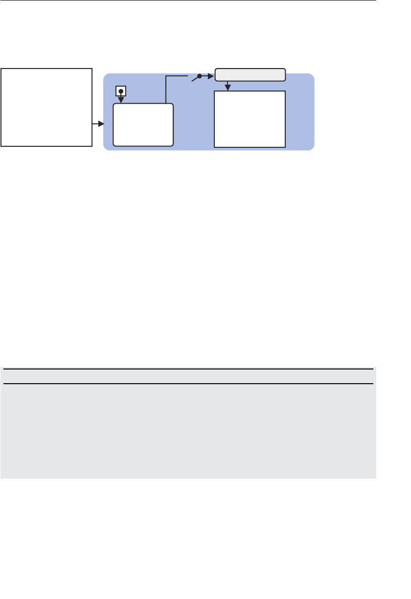
ptg11539634

Drawing Multiple Points 81

So, after executing this fourth step, the preparations are nearly completed in the WebGL

system for using the buffer object at the attribute variable specified by location . As you can

see in Figure 3.9 , although the buffer object has been assigned to the attribute variable,

WebGL requires a final step to “enable” the assignment and make the final connection.

redahSxetreV

tpircSavaJ

{)(niamnoitcnuf

…LGbeWteg=lgrav

…

;)…(retnioPbirttAxetrev.lg

…

tcejbOreffuB

REFFUB_YARRA.lg

5 . 0 , 0 . 0

5 . 0 — , 5 . 0 —

attribute variable

Figure 3.9 Assign a buffer object to an attribute variable

The fifth and final step is to enable the assignment of the buffer object to the attribute

variable.

Enable the Assignment to an Attribute Variable

(gl.enableVertexAttribArray())

To make it possible to access a buffer object in a vertex shader, we need to enable the

assignment of the buffer object to an attribute variable by using

gl.enableVertexAttrib-

Array() as shown in line 77:

77 gl.enableVertexAttribArray(a_Position);

The following shows the specification of gl.enableVertexAttribArray() . Note that we are

using the method to handle a buffer even though the method name suggests it’s only for

use with “vertex arrays.” This is not a problem and is simply a legacy from OpenGL.

gl.enableVertexAttribArray(location)

Enable the assignment of a buffer object to the attribute variable specified by location .

Parameters location Specifies the storage location of an attribute variable.

Return value None

Errors INVALID_VALUE location is greater than or equal to the maximum number

of attribute variables (8 by default).

When you execute

gl.enableVertexAttribArray() specifying an attribute variable that

has been assigned a buffer object, the assignment is enabled, and the unconnected line is

connected as shown in Figure 3.10 .

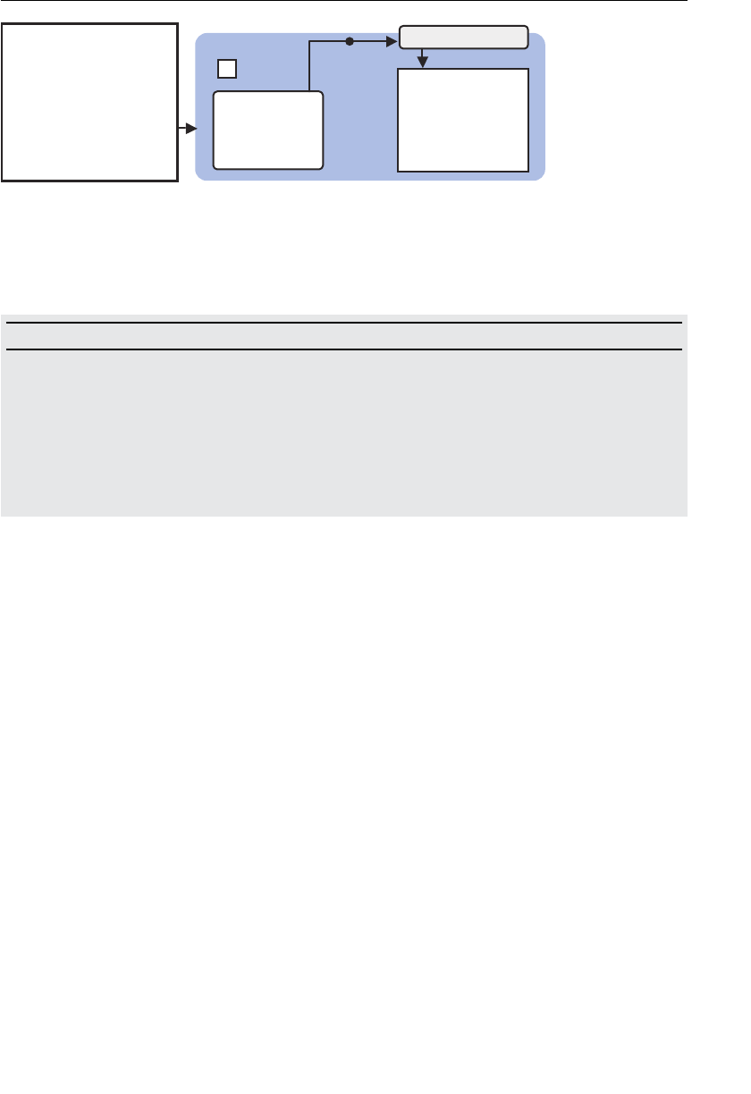
ptg11539634

CHAPTER 3 Drawing and Transforming Triangles

redahSxetreV

{)(niamnoitcnuf

…LGbeWteg=lgrav

…

tcejbOreffuB

REFFUB_YARRA.lg

5.0,0.0

5.0—,5.0—

tpircSavaJ

gl.vertexAttribArray(…);

attribute variable

Figure 3.10 Enable the assignment of a buffer object to an attribute variable

You can also break this assignment (disable it) using the method

gl.disableVertexAttribArray() .

gl.disableVertexAttribArray(location)

Disable the assignment of a buffer object to the attribute variable specified by location .

Parameters location Specifies the storage location of an attribute variable.

Return Value None

Errors INVALID_VALUE location is greater than or equal to the maximum number

of attribute variables (8 by default).

Now, everything is set! All you need to do is run the vertex shader, which draws the

points using the vertex coordinates specified in the buffer object. As in Chapter 2 , you

will use the method

gl.drawArrays , but because you are drawing multiple points, you will

actually use the second and third parameters of

gl.drawArrays() .

Note that after enabling the assignment, you can no longer use gl.vertexAttrib[1234]

f() to assign data to the attribute variable. You have to explicitly disable the assignment

of a buffer object. You can’t use both methods simultaneously.

The Second and Third Parameters of gl.drawArrays()

Before entering into a detailed explanation of these parameters, let’s take a look at the

specification of

gl.drawArrays() that was introduced in Chapter 2 . Following is a recap of

the method with only the relevant parts of the specification shown.

ptg11539634

Drawing Multiple Points 83

gl.drawArrays(mode, first, count)

Execute a vertex shader to draw shapes specified by the mode parameter.

Parameters mode Specifies the type of shape to be drawn. The following symbolic

constants are accepted:

gl.POINTS , gl.LINES , gl.LINE_STRIP , gl.

LINE_LOOP , gl.TRIANGLES , gl.TRIANGLE_STRIP , and gl.TRIANGLE_

FAN .

first Specifies what number-th vertex is used to draw from (integer).

count Specifies the number of vertices to be used (integer).

In the sample program this method is used as follows:

47 gl.drawArrays(gl.POINTS, 0, n); // n is 3

As in the previous examples, because you are simply drawing three points, the first param-

eter is still

gl.POINTS . The second parameter first is set to 0 because you want to draw

from the first coordinate in the buffer. The third parameter count is set to 3 because you

want to draw three points (in line 47,

n is 3).

When your program runs line 47, it actually causes the vertex shader to be executed count

(three) times, sequentially passing the vertex coordinates stored in the buffer object via

the attribute variable into the shader ( Figure 3.11 ).

Note that for each execution of the vertex shader, 0.0 and 1.0 are automatically supplied

to the z and w components of

a_Position because a_Position requires four components

(

vec4 ) and you are supplying only two.

Remember that at line 74, the second parameter size of g l.vertexAttribPointer() is set

to 2. As just discussed, the second parameter indicates how many coordinates per vertex

are specified in the buffer object and, because you are only specifying the x and y coordi-

nates in the buffer, you set the size value to 2:

74 gl.vertexAttribPointer(a_Position, 2, gl.FLOAT, false, 0, 0);

After drawing all points, the content of the color buffer is automatically displayed in the

browser (bottom of Figure 3.11 ), resulting in our three red points, as shown in Figure 3.2 .

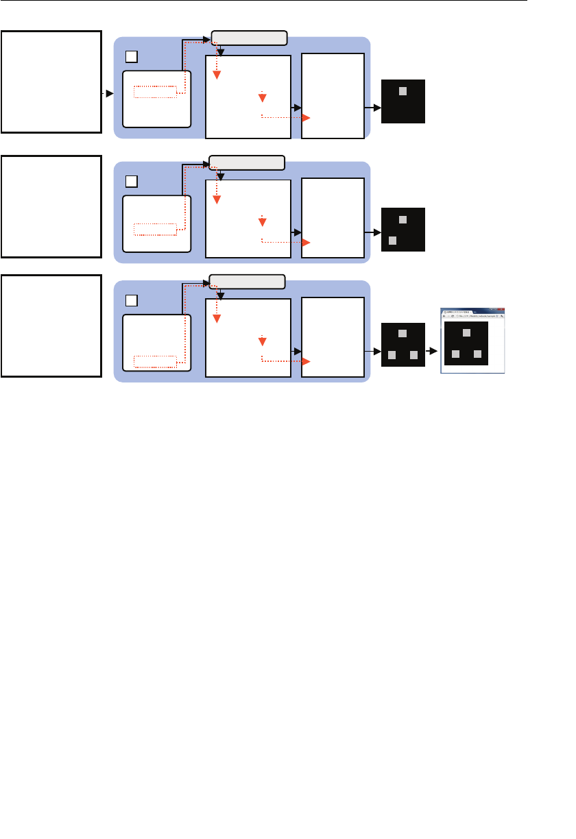
ptg11539634

CHAPTER 3 Drawing and Transforming Triangles

Experimenting with the Sample Program

Let’s experiment with the sample program to better understand how gl.drawArrays()

works by modifying the second and third parameters. First, let’s specify 1 as the third

argument for count at line 47 instead of our variable

n (set to 3) as follows:

47 gl.drawArrays(gl.POINTS, 0, 1 );

In this case, the vertex shader is executed only once, and a single point is drawn using the

first vertex in the buffer object.

If you now specify 1 as the second argument, only the second vertex is used to draw

a point. This is because you are telling WebGL that you want to start drawing from

the second vertex and you only want to draw one vertex. So again, you will see only a

single point, although this time it is the second vertex coordinates that are shown in the

browser:

47 gl.drawArrays(gl.POINTS, 1 , 1);

Vertex Shader

JavaScript

function main() {

…

var gl=getWebGL…

…

gl.drawArrays( …, 0, n);

gl.ARRAY_BUFFER attribute a_Position;

Buffer Object

0.0, 0.5

-0.5, -0.5

0.5, -0.5

Fragment

Shader

gl_Position = a_Position;

(0.0, 0.5, 0.0, 1.0)

gl_FragColor =

vec4(…);

Vertex Shader

attribute a_Position;

JavaScript

function main() {

…

var gl=getWebGL…

…

gl.drawArrays( …, 0, n);

Buffer Object

gl.ARRAY_BUFFER

0.0, 0.5

-0.5, -0.5

0.5, -0.5

Fragment

Shader

gl_Position = a_Position;

(-0.5, -0.5, 0.0, 1.0)

gl_FragColor =

vec4(…);

Vertex Shader

attribute a_Position;

JavaScript

function main() {

…

var gl=getWebGL…

…

gl.drawArrays(…, 0, n);

Buffer Object

gl.ARRAY_BUFFER

0.0, 0.5

-0.5, -0.5

0.5, -0.5

Fragment

Shader

gl_Position = a_Position;

(0.5, -0.5, 0.0, 1.0)

gl_FragColor =

vec4(…);

First Execution

Second Execution

Third Execution

Color Buffer

Browser

Figure 3.11 How the data in a buffer object is passed to a vertex shader during execution

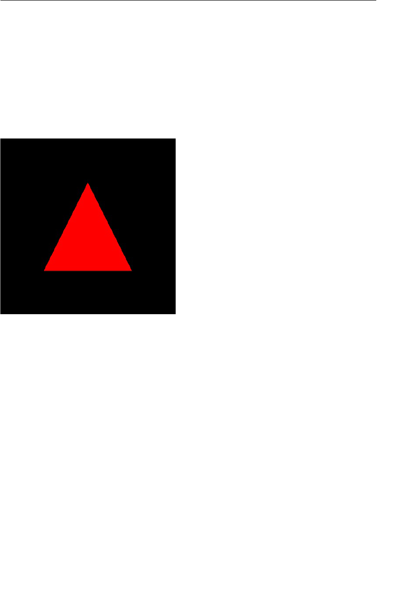
ptg11539634

Hello Triangle 85

This gives you a quick feel for the role of the parameters first and count . However, what

will be happen if you change the first parameter mode ? The next section explores the first

parameter in more detail.

Hello Triangle

Now that you’ve learned the basic techniques to pass multiple vertex coordinates to a

vertex shader, let’s try to draw other shapes using multiple vertex coordinates. This section

uses a sample program

HelloTriangle , which draws a single 2D triangle. Figure 3.12

shows a screenshot of

HelloTriangle .

Figure 3.12 HelloTriangle

Sample Program (HelloTriangle.js)

Listing 3.3 shows HelloTriangle.js , which is almost identical to MultiPoint.js used in

the previous section with two critical differences.

Listing 3.3 HelloTriangle.js

1 // HelloTriangle.js

2 // Vertex shader program

3 var VSHADER_SOURCE =

4 ‘attribute vec4 a_Position;n’ +

5 ‘void main() {n’ +

6 ‘ gl_Position = a_Position;n’ +

7 ‘}n’;

ptg11539634

CHAPTER 3 Drawing and Transforming Triangles

9 // Fragment shader program

10 var FSHADER_SOURCE =

11 ‘void main() {n’ +

12 ‘ gl_FragColor = vec4(1.0, 0.0, 0.0, 1.0);n’ +

13 ‘}n’;

15 function main() {

…

19 // Get the rendering context for WebGL

20 var gl = getWebGLContext(canvas);

…

26 // Initialize shaders

27 if (!initShaders(gl, VSHADER_SOURCE, FSHADER_SOURCE)) {

…

30 }

32 // Set the positions of vertices

33 var n = initVertexBuffers(gl);

…

39 // Set the color for clearing <canvas>

…

45 // Draw a triangle

46 gl.drawArrays(gl.TRIANGLES, 0, n);

47 }

49 function initVertexBuffers(gl) {

50 var vertices = new Float32Array([

51 0.0, 0.5, -0.5, -0.5, 0.5, -0.5

52 ]);

53 var n = 3; // The number of vertices

…

78 return n;

79 }

The two differences from MultiPoint.js are

• The line to specify the size of a point gl_PointSize = 10.0 ; has been removed from

the vertex shader. This line only has an effect when you are drawing a point.

• The first parameter of gl.drawArrays() has been changed from gl.POINTS to

gl.TRIANGLES at line 46.

The first parameter, mode, of gl.drawArrays() is powerful and provides the ability to draw

various shapes. Let’s take a look.

ptg11539634

Hello Triangle 87

Basic Shapes

By changing the argument we use for the first parameter, mode, of gl.drawArrays() , we

can change the meaning of line 46 into “execute the vertex shader three times (

n is 3),

and draw a triangle using the three vertices in the buffer, starting from the first vertex

coordinate”:

46 gl.drawArrays(gl.TRIANGLES, 0, n);

In this case, the three vertices in the buffer object are no longer individual points, but

become three vertices of a triangle.

The WebGL method

gl.drawArrays() is both powerful and flexible, allowing you to

specify seven different types of basic shapes as the first argument. These are explained in

more detail in Table 3.3 . Note that v0, v1, v2 … indicates the vertices specified in a buffer

object. The order of vertices affects the drawing of the shape.

The shapes in the table are the only ones that WebGL can draw directly, but they are the

basics needed to construct complex 3D graphics. (Remember the frog at the start of this

chapter.)

Table 3.3 Basic Shapes Available in WebGL

Basic

Shape Mode Description

Points gl.POINTS A series of points. The points are drawn at v0, v1, v2 …

Line

segments

gl.LINES A series of unconnected line segments. The individual lines

are drawn between vertices given by (v0, v1), (v2, v3), (v4,

v5)… If the number of vertices is odd, the last one is ignored.

Line strips

gl.LINE_STRIP A series of connected line segments. The line segments are

drawn between vertices given by (v0, v1), (v1, v2), (v2, v3), …

The first vertex becomes the start point of the first line, the

second vertex becomes the end point of the first line and the

start point of the second line, and so on. The i -th ( i > 1) vertex

becomes the start point of the i -th line and the end point of

the i-1 -th line. (The last vertex becomes the end point of the

last line.)

Line loops

gl.LINE_LOOP A series of connected line segments. In addition to the lines

drawn by

gl.LINE_STRIP , the line between the last vertex and

the first vertex is drawn. The line segments drawn are (v0, v1),

(v1, v2), …, and (v n , v0). v n is the last vertex.

Triangles

gl.TRIANGLES A series of separate triangles. The triangles given by vertices

(v0, v1, v2), (v3, v4, v5), … are drawn. If the number of verti-

ces is not a multiple of 3, the remaining vertices are ignored.

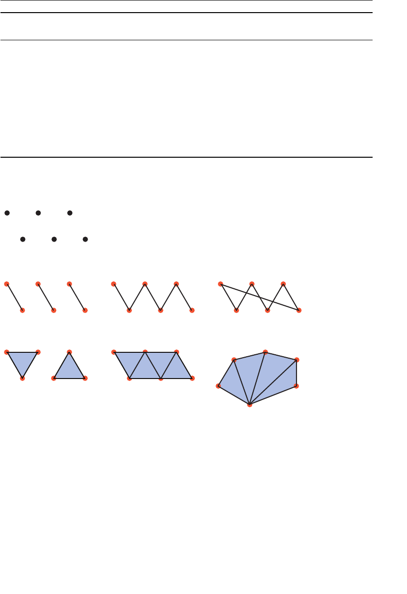
ptg11539634

CHAPTER 3 Drawing and Transforming Triangles

Basic

Shape Mode Description

Triangle

strips

gl.TRIANGLE_

STRIP

A series of connected triangles in strip fashion. The first three

vertices form the first triangle and the second triangle is

formed from the next vertex and one of the sides of the first

triangle. The triangles are drawn given by (v0, v1, v2), (v2, v1,

v3), (v2, v3, v4) … (Pay attention to the order of vertices.)

Triangle

fans

gl.TRIANGLE_

FAN

A series of connected triangles sharing the first vertex in fan-

like fashion. The first three vertices form the first triangle and

the second triangle is formed from the next vertex, one of the

sides of the first triangle, and the first vertex. The triangles are

drawn given by (v0, v1, v2), (v0, v2, v3), (v0, v3, v4), …

Figure 3.13 shows these basic shapes.

STNIOP.lg

POOL_ENIL.lgPIRTS_ENIL.lgSENIL.lg

NAF_ELGNAIRT.lgPIRTS_ELGNAIRT.lgSELGNAIRT.lg

Figure 3.13 Basic shapes available in WebGL

As you can see from the figure, WebGL can draw only three types of shapes: a point, a

line, and a triangle. However, as explained at the beginning of this chapter, spheres to

cubes to 3D monsters to humanoid characters in a game can be constructed from small

triangles. Therefore, you can use these basic shapes to draw anything.

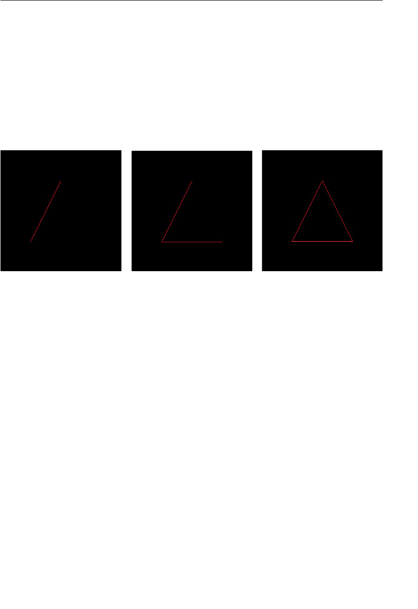
ptg11539634

Hello Triangle 89

Experimenting with the Sample Program

To examine what will happen when using gl.LINES , gl.LINE_STRIP , and gl.LINE_LOOP ,

let’s change the first argument of

gl.drawArrays( ) as shown next. The name of each

sample program is

HelloTriangle _ LINES , HelloTriangle_LINE_STRIP , and HelloTriangle_

LINE_LOOP , respectively:

46 gl.drawArrays( gl.LINES , 0, n);

46 gl.drawArrays( gl.LINE_STRIP , 0, n);

46 gl.drawArrays( gl.LINE_LOOP , 0, n);

Figure 3.14 shows a screenshot of each program.

Figure 3.14 gl.LINES, gl.LINE_STRIP, and gl.LINE_LOOP

As you can see,

gl.LINES draws a line using the first two vertices and does not use the

last vertex, whereas

gl.LINE_STRIP draws two lines using the first three vertices. Finally,

gl.LINE_LOOP draws the lines in the same manner as gl.LINE_STRIP but then “loops”

between the last vertex and the first vertex and makes a triangle.

Hello Rectangle (HelloQuad)

Let’s use this basic way of drawing triangles to draw a rectangle. The name of the sample

program is

HelloQuad , and Figure 3.15 shows a screenshot when it’s loaded into your

browser.

Figure 3.16 shows the vertices of the rectangle. Of course, the number of vertices is four

because it is a rectangle. As explained in the previous section, WebGL cannot draw a rect-

angle directly, so you need to divide the rectangle into two triangles (v0, v1, v2) and (v2,

v1, v3) and then draw each one using

gl.TRIANGLES , gl.TRIANGLE_STRIP , or gl.TRIANGLE_

FAN . In this example, you’ll use gl.TRIANGLE_STRIP because it only requires you to specify

four vertices. If you were to use

gl.TRIANGLES , you would need to specify a total of six.

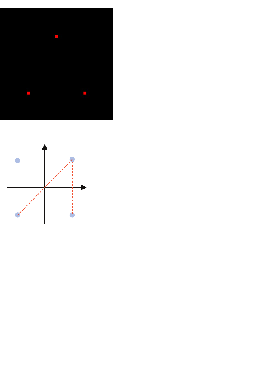
ptg11539634

CHAPTER 3 Drawing and Transforming Triangles

)0.0 ,5.0— ,5.0(

)0.0 ,5.0 ,5.0—(

)0.0 ,5.0 ,5.0(

)0.0 ,5.0— ,5.0—(

Figure 3.16 The four vertex coordinates of the rectangle

Basing the example on

HelloTriangle.js , you need to add an extra vertex coordinate

at line 50. Pay attention to the order of vertices; otherwise, the draw command will not

execute correctly:

50 var vertices = new Float32Array([

51 -0.5, 0.5, -0.5, -0.5, 0.5, 0.5, 0.5, -0.5

52 ]);

Because you’ve added a fourth vertex, you need to change the number of vertices from 3

to 4 at line 53:

53 var n = 4; // The number of vertices

Figure 3.15 HelloQuad

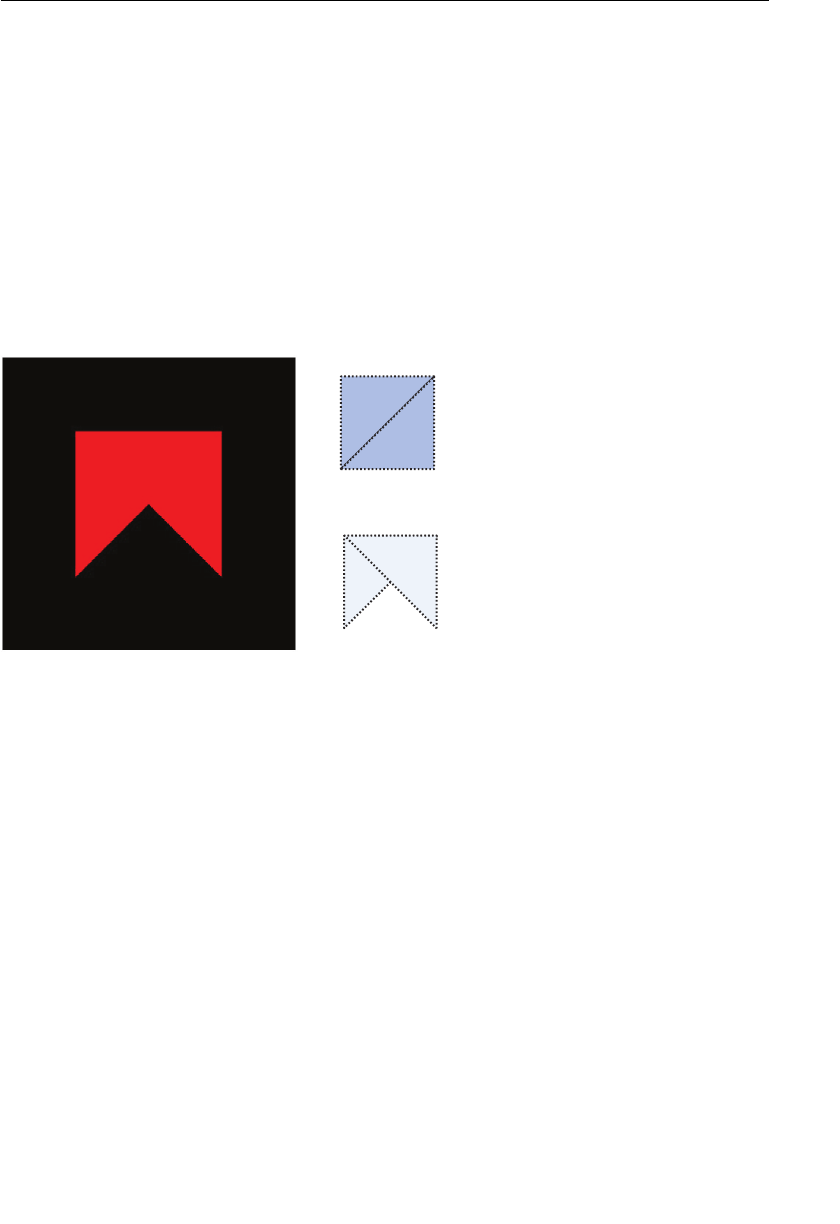
ptg11539634

Moving, Rotating, and Scaling 91

Then, by modifying line 46 as follows, your program will draw a rectangle in the browser:

46 gl.drawArrays( gl.TRIANGLE_STRIP , 0, n);

Experimenting with the Sample Program

Now that you have a feel for how to use gl.TRIANGLE_STRIP , let’s change the first

parameter of

gl.drawArrays() to gl.TRIANGLE_FAN . The name of the sample program is

HelloQuad_FAN :

46 gl.drawArrays( gl.TRIANGLE_FAN , 0, n);

Figure 3.17 show a screenshot of HelloQuad_FAN . In this case, we can see the ribbon-like

shape on the screen.

PIRTS_ELGNAIRT.lg

NAF_ELGNAIRT.lg

Figure 3.17 HelloQuad_FAN

Looking at the order of vertices and the triangles drawn by

gl.TRIANGLE_FAN shown on

the right side of Figure 3.17 , you can see why the result became a ribbon-like shape.

Essentially,

gl.TRIANGLE_FAN causes WebGL to draw a second triangle that shares the first

vertex (v0), and this second triangle overlaps the first, creating the ribbon-like effect.

Moving, Rotating, and Scaling

Now that you understand the basics of drawing shapes like triangles and rectangles, let’s

take another step and try to move (translate), rotate, and scale the triangle and display the

results on the screen. These operations are called transformations (affine transforma-

tions) . This section introduces some math to explain each transformation and help you

to understand how each operation can be realized. However, when you write your own

programs, you don’t need the math; instead, you can use one of several convenient librar-

ies, explained in the next section, that handle the math for you.

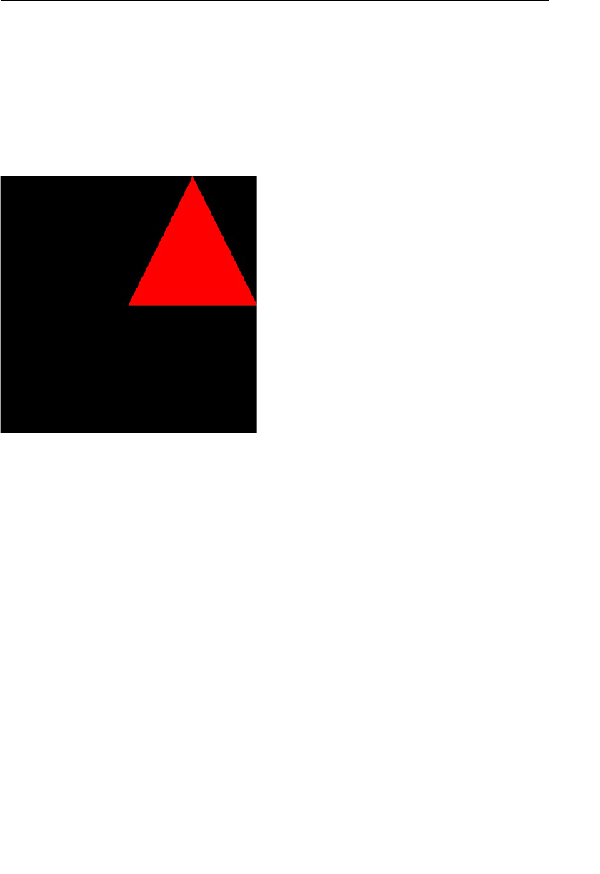
ptg11539634

CHAPTER 3 Drawing and Transforming Triangles

If you find reading this section and in particular the math too much on first read, it’s

okay to skip it and return later. Or, if you already know that transformations can be

written using a matrix, you can skip this section as well.

First, let’s write a sample program,

TranslatedTriangle , that moves a triangle 0.5 units

to the right and 0.5 units up. You can use the triangle you drew in the previous section.

The right direction means the positive direction of the x-axis, and the up direction means

the positive direction of the y-axis. (See the coordinate system in Chapter 2 .) Figure 3.18

shows

TranslatedTriangle .

Figure 3.18 TranslatedTriangle

Translation

Let us examine what kind of operations you need to apply to each vertex coordinate

of a shape to translate (move) the shape. Essentially, you just need to add a translation

distance for each direction (x and y) to each component of the coordinates. Looking at

Figure 3.19 , the goal is to translate the point p (x, y, z) to the point p’ (x’, y’, z’), so the

translation distance for the x, y, and z direction is

Tx , Ty , and Tz , respectively. In this

figure,

Tz is 0.

To determine the coordinates of p’, you simply add the T values, as shown in

Equation 3.1 .

Equation 3.1

x’ = x + Tx

y’ = y + Ty

z’ = z + Tz

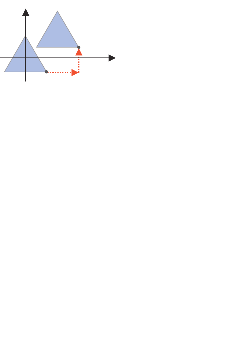
ptg11539634

Moving, Rotating, and Scaling 93

These simple equations can be implemented in a WebGL program just by adding each

constant value to each vertex coordinate. You’ve probably realized already that because

they are a per-vertex operation , you need to implement the operations in a vertex

shader. Conversely, they clearly aren’t a per-fragment operation, so you don’t need to

worry about the fragment shader.

Once you understand this explanation, implementation is easy. You need to pass the

translation distances

Tx , Ty , and Tz to the vertex shader, apply Equation 3.1 using the

distances, and then assign the result to

gl_Position . Let’s look at a sample program that

does this.

Sample Program (TranslatedTriangle.js)

Listing 3.4 shows TranslatedTriangle.js , in which the vertex shader is partially modi-

fied to carry out the translation operation. However, the fragment shader is the same as

HelloTriangle.js in the previous section. To support the modification to the vertex

shader, some extra code is added to the

main() function in the JavaScript.

Listing 3.4 TranslatedTriangle.js

1 // TranslatedTriangle.js

2 // Vertex shader program

3 var VSHADER_SOURCE =

4 ‘attribute vec4 a_Position;n’ +

5 ‘uniform vec4 u_Translation;n’ +

6 ‘void main() {n’ +

7 ‘ gl_Position = a_Position + u_Translation;n’ +

8 ‘}n’;

10 // Fragment shader program

…

)‘z,‘y,‘x(‘p

)z,y,x(p

Figure 3.19 Calculating translation distances

ptg11539634

CHAPTER 3 Drawing and Transforming Triangles

16 // The translation distance for x, y, and z direction

17 var Tx = 0.5, Ty = 0.5, Tz = 0.0;

19 function main() {

…

23 // Get the rendering context for WebGL

24 var gl = getWebGLContext(canvas);

…

30 // Initialize shaders

31 if (!initShaders(gl, VSHADER_SOURCE, FSHADER_SOURCE)) {

…

34 }

36 // Set the positions of vertices

37 var n = initVertexBuffers(gl);

…

43 // Pass the translation distance to the vertex shader

44 var u_Translation = gl.getUniformLocation(gl.program, ‘u_Translation’);

…

49 gl.uniform4f(u_Translation, Tx, Ty, Tz, 0.0);

51 // Set the color for clearing <canvas>

…

57 // Draw a triangle

58 gl.drawArrays(gl.TRIANGLES, 0, n);

59 }

61 function initVertexBuffers(gl) {

62 var vertices = new Float32Array([

63 0.0.0, 0.5, -0.5, -0.5, 0.5, -0.5

64 ]);

65 var n = 3; // The number of vertices

…

90 return n;

93 }

First, let’s examine main() in JavaScript. Line 17 defines the variables for each translation

distance of Equation 3.1 :

17 var Tx = 0.5, Ty = 0.5, Tz = 0.0;

Because Tx , Ty , and Tz are fixed (uniform) values for all vertices, you use the uniform vari-

able

u_Translation to pass them to a vertex shader. Line 44 retrieves the storage location

of the uniform variable, and line 49 assigns the data to the variable:

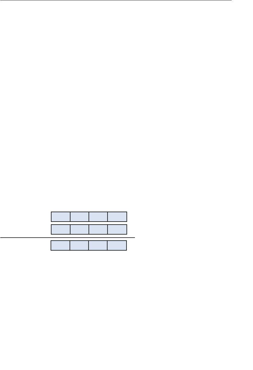
ptg11539634

Moving, Rotating, and Scaling 95

44 var u_Translation = gl.getUniformLocation(gl.program, ‘u_Translation’);

…

49 gl.uniform4f(u_Translation, Tx, Ty, Tz, 0.0);

Note that gl.uniform4f() requires a homogenous coordinate, so we supply a fourth argu-

ment (w) of 0.0. This will be explained in more detail later in this section.

Now, let’s take a look at the vertex shader that uses this translation data. As you can see,

the uniform variable

u_Translation in the shader, to which the translation distances

are passed, is defined as type

vec4 at line 5. This is because you want to add the compo-

nents of

u_Translation to the vertex coordinates passed to a_Position (as defined by

Equation 3.1 ) and then assign the result to the variable

gl_Position , which has type

vec4 . Remember, per Chapter 2 , that the assignment operation in GLSL ES is only allowed

between variables of the same types:

4 ‘attribute vec4 a_Position;n’ +

5 ‘uniform vec4 u_Translation;n’ +

6 ‘void main() {n’ +

7 ‘ gl_Position = a_Position + u_Translation;n’ +

8 ‘}n’;

After these preparations have been completed, the rest of tasks are straightforward. To

calculate Equation 3.1 within the vertex shader, you just add each translation distance

(Tx, Ty, Tz) passed in

u_Translation to each vertex coordinate (x, y, z) passed in

a_Position .

Because both variables are of type vec4 , you can use the + operator, which will actually

add the four components simultaneously (see Figure 3.20 ). This easy addition of vectors is

a feature of GLSL ES and will be explained in more detail in Chapter 6 .

noitisoP_a4cev

noitalsnarT_u4cev

x1 y1 z1 w1

x1+x2 y1+y2 z1+z2 w1+w2

x2 y2 z2 w2

Figure 3.20 Addition of vec4 variables

Now, we’ll return to the fourth element, (w), of the vector. As explained in Chapter 2 , you

need to specify the homogeneous coordinate to

gl_Position , which is a four-dimensional

coordinate. If the last component of the homogeneous coordinate is 1.0, the coordinate

indicates the same position as the three-dimensional coordinate. In this case, because the

last component is

w1+w2 to ensure that w1+w2 is 1.0, you need to specify 0.0 to the value of

w (the fourth parameter of

gl.uniform4f() ).

ptg11539634

CHAPTER 3 Drawing and Transforming Triangles

Finally, at line 58, gl.drawArrays(gl.TRIANGLES, 0, n) executes the vertex shader. For

each execution, the following three steps are performed:

1. Each vertex coordinate set is passed to

a_Position .

u_Translation is added to a_Position .

3. The result is assigned to gl_Position .

Once executed, you’ve achieved your goal because each vertex coordinate set is modi-

fied (translated), and then the translated shape (in this case, a triangle) is displayed on

the screen. If you now load

TranslatedTriangle.html into your browser, you will see the

translated triangle.

Now that you’ve mastered translation (moving), the next step is to look at rotation. The

basic approach to realize rotation is the same as translation, requiring you to manipulate

the vertex coordinates in the vertex shader.

Rotation

Rotation is a little more complex than translation because you have to specify multiple

items of information. The following three items are required:

• Rotation axis (the axis the shape will be rotated around)

• Rotation direction (the direction: clockwise or counterclockwise)

• Rotation angle (the number of degrees the shape will be rotated through)

In this section, to simplify the explanation, you can assume that the rotation is performed

around the

z -axis, in a counterclockwise direction, and for β degrees. You can use the

same approach to implement other rotations around the x-axis or y-axis.

In the rotation, if β is positive, the rotation is performed in a counterclockwise direction

around the rotation axis looking at the shape toward the negative direction of the z-axis

(see Figure 3.21 ); this is called positive rotation . Just as for the coordinate system, your

hand can define the direction of rotation. If you take your right hand and have your

thumb follow the direction of the rotation axis, your fingers show the direction of rota-

tion. This is called the right-hand-rule rotation . As we discussed in Chapter 2 , it’s the

default we are using for WebGL in this book.

Now let’s find the expression to calculate the rotation in the same way that you did for

translation. As shown in Figure 3.22 , we assume that the point p’ (x’, y’, z’) is the β degree

rotated point of p (x, y, z) around the z-axis. Because the rotation is around the z-axis, the

z coordinate does not change, and you can ignore it for now. The explanation is a little

mathematical, so let’s take it a step at a time.

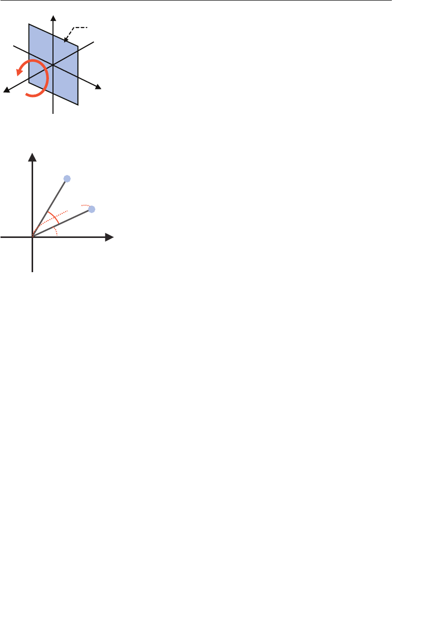
ptg11539634

Moving, Rotating, and Scaling 97

ｒ

)‘z,‘y,‘x(‘p

)z,y,x(p

Figure 3.22 Calculating rotation around the z-axis

In Figure 3.22 ,

r is the distance from the origin to the point p , and α is the rotation angle

from the x-axis to the point. You can use these items of information to represent the coor-

dinates of

p , as shown in Equation 3.2 .

Equation 3.2

x = r cos α

y = r sin α

Similarly, you can find the coordinate of p’ by using

r , α, and β as follows:

x’ = r cos (α +

β )

y’ = r sin (α +

β )

Screen

Figure 3.21 Positive rotation around the z-axis

ptg11539634

CHAPTER 3 Drawing and Transforming Triangles

Then you can use the addition theorem of trigonometric functions

1 to get the following:

x’ = r (cos α cos β – sin α sin β)

y’ = r (sin α cos β + cos α sin β)

Finally, you get the following expressions ( Equation 3.3 ) by assigning Equation 3.2 to the

previous expressions and removing

r and α.

Equation 3.3

x’ = x cos β – y sin β

y’ = x sin β + y cos β

z’ = z

So by passing the values of sin β and cos β to the vertex shader and then calculating

Equation 3.3 in the shader, you get the coordinates of the rotated point. To calculate sin β

and cos β, you can use the methods of the JavaScript

Math object.

Let’s look at a sample program, RotatedTriangle , which rotates a triangle around the

z-axis, in a counterclockwise direction, by 90 degrees. Figure 3.23 shows

RotatedTriangle .

Figure 3.23 RotatedTriangle

1 sin(a ± b) = sin a cos b ∓ cos a sin b

cos(a ± b) = cos a cos b ∓ sin a sin b

ptg11539634

Moving, Rotating, and Scaling 99

Sample Program (RotatedTriangle.js)

Listing 3.5 shows RotatedTriangle.js which, in a similar manner to

TranslatedTriangle . js , modifies the vertex shader to carry out the rotation operation.

The fragment shader is the same as in

TranslatedTriangle.js and, as usual, is not shown.

Again, to support the shader modification, several processing steps are added to

main() in

the JavaScript program. Additionally, Equation 3.3 is added in the comments from lines 4

to 6 to remind you of the calculation needed.

Listing 3.5 RotatedTriangle.js

1 // RotatedTriangle.js

2 // Vertex shader program

3 var VSHADER_SOURCE =

4 // x’ = x cos b — y sin b

5 // y’ = x sin b + y cos b Equation 3.3

6 // z’ = z

7 ‘attribute vec4 a_Position;n’ +

8 ‘uniform float u_CosB, u_SinB;n’ +

9 ‘void main() {n’ +

10 ‘ gl_Position.x = a_Position.x * u_CosB — a_Position.y *u_SinB;n’+

11 ‘ gl_Position.y = a_Position.x * u_SinB + a_Position.y * u_CosB;n’+

12 ‘ gl_Position.z = a_Position.z;n’ +

13 ‘ gl_Position.w = 1.0;n’ +

14 ‘}n’;

16 // Fragment shader program

…

22 // Rotation angle

23 var ANGLE = 90.0;

25 function main() {

…

42 // Set the positions of vertices

43 var n = initVertexBuffers(gl);

…

49 // Pass the data required to rotate the shape to the vertex shader

50 var radian = Math.PI * ANGLE / 180.0; // Convert to radians

51 var cosB = Math.cos(radian);

52 var sinB = Math.sin(radian);

54 var u_CosB = gl.getUniformLocation(gl.program, ‘u_CosB’);

55 var u_SinB = gl.getUniformLocation(gl.program, ‘u_SinB’);

…

ptg11539634

CHAPTER 3 Drawing and Transforming Triangles

100

60 gl.uniform1f(u_CosB, cosB);

61 gl.uniform1f(u_SinB, sinB);

63 // Set the color for clearing <canvas>

…

69 // Draw a triangle

70 gl.drawArrays(gl.TRIANGLES, 0, n);

71 }

73 function initVertexBuffers(gl) {

74 var vertices = new Float32Array([

75 0.0, 0.5, -0.5, -0.5, 0.5, -0.5

76 ]);

77 var n = 3; // The number of vertices

…

105 return n;

106 }

Let’s look at the vertex shader, which is straightforward:

2 // Vertex shader program

3 var VSHADER_SOURCE =

4 // x’ = x cos b — y sin b

5 // y’ = x sin b + y cos b

6 // z’ = z

7 ‘attribute vec4 a_Position;n’ +

8 ‘uniform float u_CosB, u_SinB;n’ +

9 ‘void main() {n’ +

10 ‘ gl_Position.x = a_Position.x * u_CosB — a_Position.y * u_SinB;n’+

11 ‘ gl_Position.y = a_Position.x * u_SinB + a_Position.y * u_CosB;n’+

12 ‘ gl_Position.z = a_Position.z;n’ +

13 ‘ gl_Position.w = 1.0;n’ +

14 ‘}n’;

Because the goal is to rotate the triangle by 90 degrees, the sine and cosine of 90 need to

be calculated. Line 8 defines two uniform variables for receiving these values, which are

calculated in the JavaScript program and then passed to the vertex shader.

You could pass the rotation angle to the vertex shader and then calculate the values of

sine and cosine in the shader. However, because they are identical for all vertices, it is

more efficient to do it once in the JavaScript.

The name of these uniform variables,

u_CosB and u_SinB , are defined following the

naming rule used throughout this book. As you will remember, you use the uniform vari-

able because the values of these variables are uniform (unchanging) per vertex.

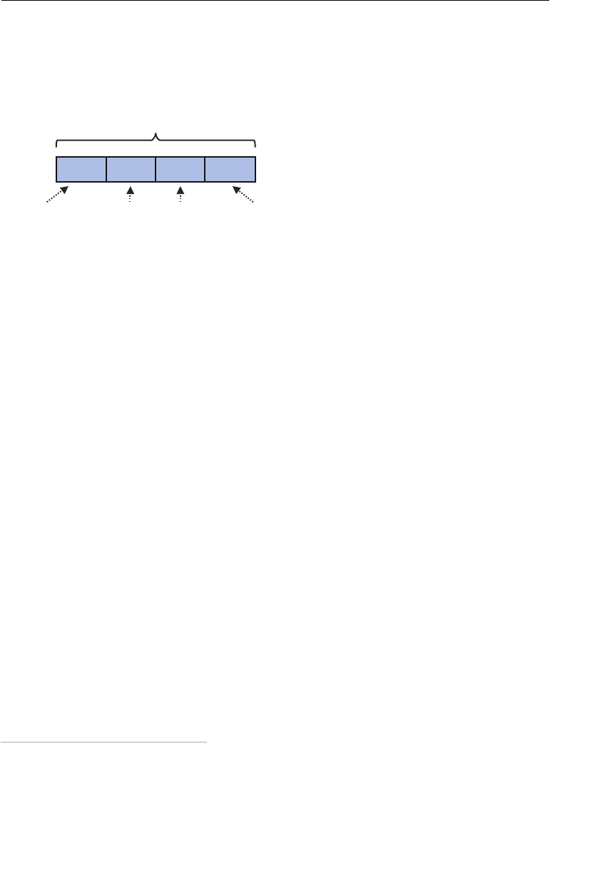
ptg11539634

Moving, Rotating, and Scaling 101

As in the previous sample programs, x, y, z, and w are passed in a group to the attribute

variable

a_Position in the vertex shader. To apply Equation 3.3 to x, y, and z, you need

to access each component in

a_Position separately. You can do this easily using the .

operator, such as

a_Position.x , a_Position.y , and a_Position.z (see Figure 3.24 and

Chapter 6 ).

noitisoP_a4cev

w.noitisoP_az.noitisoP_ay.noitisoP_ax.noitisoP_a

xyzw

Figure 3.24 Access methods for each component in a vec4

Handily, you can use the same operator to access each component in

gl_Position to

which the vertex coordinate is written, so you can calculate x’ = x cos β – y sin β from

Equation 3.3 as shown at line 10:

10 ‘ gl_Position.x = a_Position.x * u_CosB — a_Position.y * u_SinB;n’+

Similarly, you can calculate y’ as follows:

11 ‘ gl_Position.y = a_Position.x * u_SinB + a_Position.y * u_CosB;n’+

According to Equation 3.3 , you just need to assign the original z coordinate to z’ directly

at line 12. Finally, you need to assign 1.0 to the last component

2 :

12 ‘ gl_Position.z = a_Position.z;n’ +

13 ‘ gl_Position.w = 1.0;n’ +

Now look at main() in the JavaScript code, which starts from line 25. This code is mostly

the same as in

TranslatedTriangle.js . The only difference is passing cos β and sin β to

the vertex shader. To calculate the sine and cosine of β, you can use the JavaScript

Math.

sin() and Math.cos() methods. However, these methods expect parameters in radians,

not degrees, so you need to convert from degrees to radians by multiplying the number

of degrees by pi and then dividing by 180. You can utilize

Math.PI as the value of pi as

shown at line 50, where the variable

ANGLE is defined as 90 (degrees) at line 23:

50 var radian = Math.PI * ANGLE / 180.0; // Converts degrees to radians

2 In this program, you can also write gl_Position.w = a_Position.w; because a_Position.w

is 1.0.

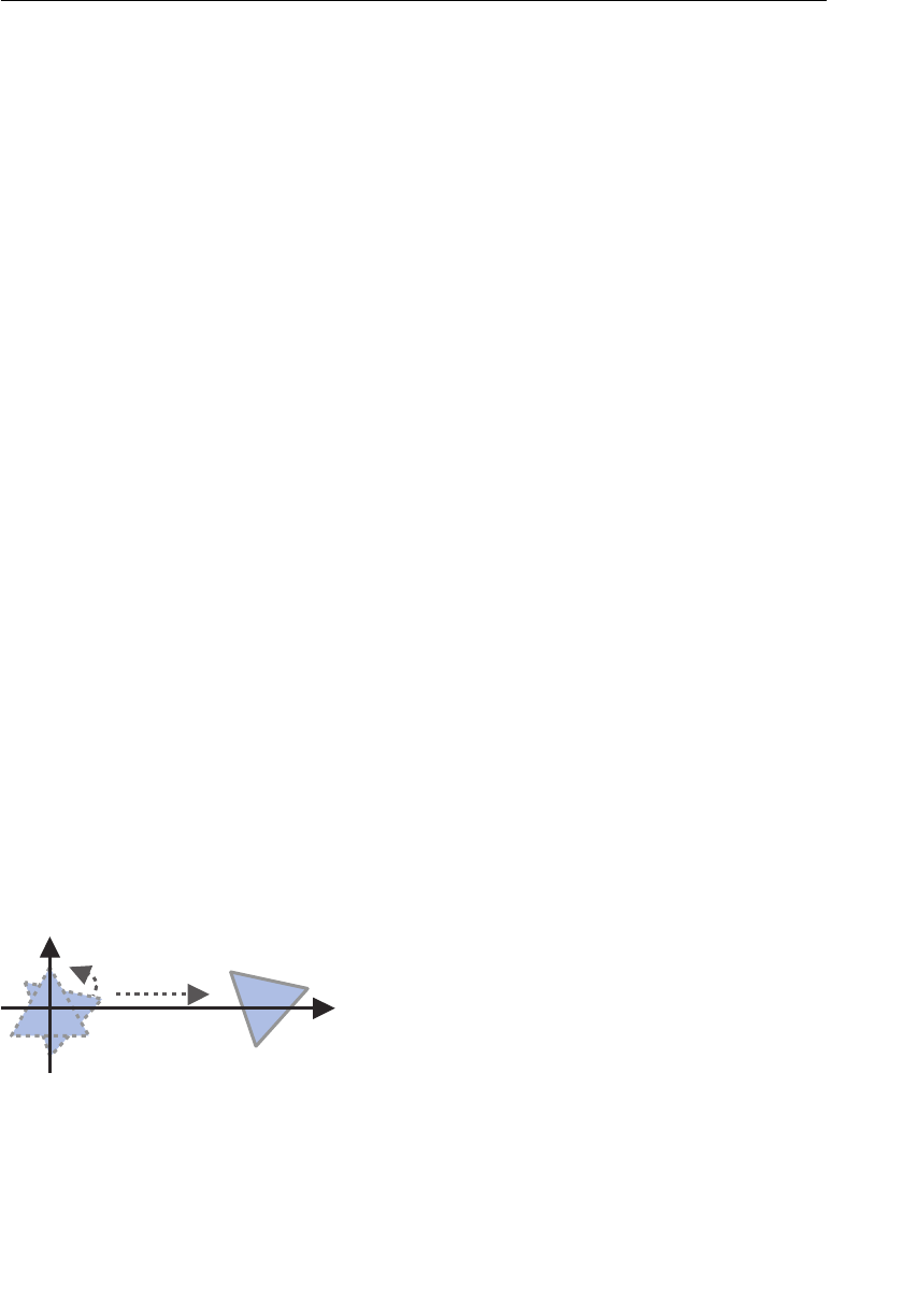
ptg11539634

CHAPTER 3 Drawing and Transforming Triangles

102

Once you have the angle in radians, lines 51 and 52 calculate cos β and sin β, and then

lines 60 and 61 pass them to the uniform variables in the vertex shader:

51 var cosB = Math.cos(radian);

52 var sinB = Math.sin(radian);

54 var u_CosB = gl.getUniformLocation(gl.program, ‘u_CosB’);

55 var u_SinB = gl.getUniformLocation(gl.program, ‘u_SinB’);

…

60 gl.uniform1f(u_CosB, cosB);

61 gl.uniform1f(u_SinB, sinB);

When you load this program into your browser, you can see the triangle, rotated through

90 degrees, on the screen. If you specify a negative value to

ANGLE , you can rotate the

triangle in the opposite direction (clockwise). You can also use the same equation. For

example, to rotate the triangle in the clockwise direction, you can specify –90 instead of

90 at line 23, and

Math.cos() and Math.sin() will deal with the remaining tasks for you.

For those of you concerned with speed and efficiency, the approach taken here (using two

uniform variables to pass the values of cos β and sin β) isn’t optimal. To pass the values as

a group, you can define the uniform variable as follows:

uniform vec2

u_CosBSinB

;

and then pass the values by:

gl.uniform2f(

u_CosBSinB,cosB, sinB

);

Then in the vertex shader, you can access them using u_CosBSinB.x and u_CosBSinB.y .

Transformation Matrix: Rotation

For simple transformations, you can use mathematical expressions. However, as your

needs become more complex, you’ll quickly find that applying a series of equations

becomes quite complex. For example a “translation after rotation” as shown in Figure 3.25

can be realized by using Equations 3.1 and 3.3 to find the new mathematical expressions

for the transformation and then implementing them in a vertex shader.

)1(

)2(

Figure 3.25 Rotate first and then translate a triangle

ptg11539634

Moving, Rotating, and Scaling 103

However, it is time consuming to determine the mathematical expressions every time

you need a new set of transformation and then implement them in a vertex shader.

Fortunately, there is another tool in the mathematical toolbox, the transformation

matrix , which is excellent for manipulating computer graphics.

As shown in Figure 3.26 , a matrix is a rectangular array of numbers arranged in rows (in

the horizontal direction) and columns (in the vertical direction). This notation makes it

easy to write the calculations explained in the previous sections. The brackets indicate

that these numbers are a group.

830

436

326

⎡⎤

⎢⎥

⎣⎦

Figure 3.26 Example of a matrix

Before explaining the details of how to use a transformation matrix to replace the equa-

tions used here, you need to make sure you understand the multiplication of a matrix and

a vector. A vector is an object represented by an n-tuple of numbers, such as the vertex

coordinates (0.0, 0.5, 1.0).

The multiplication of a matrix and a vector can be written as shown in Equation 3.4 .

(Although the multiply operator × is often omitted, we explicitly write the operator in this

book for clarity.) Here, our new vector (on the left) is the result of multiplying a matrix

(in the center) by our original vector (on the right). Note that matrix multiplication is

noncommutative. In other words, A × B is not the same as B × A. We discuss this further

in Chapter 6 .

Equation 3.4

‘

xabcx

ydefy

zghiz

⎡⎤⎡ ⎤⎡⎤

⎢⎥⎢ ⎥⎢⎥

=×

⎢⎥⎢ ⎥⎢⎥

⎣⎦⎣ ⎦⎣⎦

This matrix has three rows and three columns and is called a 3×3 matrix. The rightmost

part of the equation is a vector composed of x, y, and z. (In the case of a multiplication

of a matrix and vector, the vector is written vertically, but it has the same meaning as

when it is written horizontally.) This vector has three elements, so it is called a three-

dimensional vector. Again, the brackets on both sides of the array of numbers (vector)

are also just notation for recognizing that these numbers are a group.

In this case, x’, y’, and z’ are defined using the elements of the matrix and the vector,

as shown by Equation 3.5 . Note that the multiplication of a matrix and vector can be

ptg11539634

CHAPTER 3 Drawing and Transforming Triangles

104

defined only if the number of columns in a matrix matches the number of rows in a

vector.

Equation 3.5

x’ = ax + by + cz

y’ = dx + ey + fz

z’ = gx + hy + iz

Now, to understand how to use a matrix instead of our original equations, let’s compare

the matrix equations and Equation 3.3 (shown again as Equation 3.6 ).

Equation 3.6

x’ = x cos β – y sin β

y’ = x sin β + y cos β

z’ = z

For example, compare the equation for x’:

x’ = ax + by + cz

x’ = x cos β – y sin β

In this case, if you set a = cos β, b = -sin β, and c = 0, the equations become the same.

Similarly, let us compare the equation for y’:

y’ = dx + ey + fz

y’ = x sin β + y cos β

In this case, if you set d = sin β, e = cos β, and f = 0, you get the same equation. The last

equation about z’ is easy. If you set g = 0, h = 0, and i = 1, you get the same equation.

Then, by assigning these results to Equation 3.4 , you get Equation 3.7 .

Equation 3.7

ββ

⎡

⎣

⎢

⎤

⎦

⎥

−

⎡

⎣

⎢

⎤

⎦

⎥

⎡

⎣

⎢

⎤

⎦

⎥

‘

cos sin 0

sin cos 0

001

This matrix is called a transformation matrix because it “transforms” the right-side

vector (x, y, z) to the left-side vector (x’, y’, z’). The transformation matrix representing a

rotation is called a rotation matrix .

ptg11539634

Moving, Rotating, and Scaling 105

You can see that the elements of the matrix in Equation 3.7 are an array of coefficients in

Equation 3.6 . Once you become accustomed to matrix notation, it is easier to write and

use matrices than to have to deal with a set of transformation equations.

As you would expect, because matrices are used so often in 3DCG, multiplication of a

matrix and a vector is easy to implement in shaders. However, before exploring how, let’s

quickly look at other types of transformation matrices, and then we will start to use them

in shaders.

Transformation Matrix: Translation

Obviously, if we can use a transformation matrix to represent a rotation, we should be

able to use it for other types of transformation, such as translation. For example, let us

compare the equation for x’ in Equation 3.1 to that in Equation 3.5 as follows:

x’ = ax + by + cz — — — from Equation (3.5)

x’ = x + T

x — — — from Equation (3.1)

Here, the second equation has the constant term T

x , but the first one does not, meaning

that you cannot deal with the second one by using the 3×3 matrix of the first equation.

To solve this problem, you can use a 4×4 matrix and the fourth components of the coor-

dinate, which are set to 1 to introduce the constant terms. That is to say, we assume that

the coordinates of point p are (x, y, z, 1), and the coordinates of the translated point p (p’)

are (x’, y’, z’, 1). This gives us Equation 3.8 .

Equation 3.8

⎡

⎣

⎢

⎤

⎦

⎥

⎡

⎣

⎢

⎤

⎦

⎥

⎡

⎣

⎢

⎤

⎦

⎥

abcd

efgh

ijkl

mnop

‘

This multiplication is defined as follows:

Equation 3.9

x’ = ax + by + cz +d

y’ = ex + fy + gz + h

z’ = ix + jy + kz + l

1 = mx + ny + oz+ p

ptg11539634

CHAPTER 3 Drawing and Transforming Triangles

106

From the equation1 = mx + ny + oz + p, it is easy to find that the coefficients are m = 0,

n = 0, o = 0, and p = 1. In addition, these equations have the constant terms d, h, and l,

which look helpful to deal with Equation 3.1 because it also has constant terms. Let us

compare Equation 3.9 and Equation 3.1 (translation), which is reproduced again:

x’ = x + T

y’ = y + T

z’ = z + T

When you compare the x’ component of both equations, you can see that a=1, b=0, c=0,

and d=T

x . Similarly, when comparing y’ from both equations, you find e = 0, f = 1, g = 0,

and h = T

y ; when comparing z’ you see i=0, j=0, k=1, and l =T

z . You can use these results

to write a matrix that represents a translation, called a translation matrix , as shown in

Equation 3.10 .

Equation 3.10

⎡

⎣

⎢

⎤

⎦

⎥

⎡

⎣

⎢

⎤

⎦

⎥

⎡

⎣

⎢

⎤

⎦

⎥

‘

100

010

001

000 1 1

Rotation Matrix, Again

At this stage you have successfully created a rotation and a translation matrix, which are

equivalent to the two equations you used in the example programs earlier. The final step

is to combine these two matrices; however, the rotation matrix (3×3 matrix) and trans-

formation matrix (4×4 matrix) have different numbers of elements. Unfortunately, you

cannot combine matrices of different sizes, so you need a mechanism to make them the

same size.

To do that, you need to change the rotation matrix (3×3 matrix) into a 4×4 matrix. This is

straightforward and requires you to find the coefficient of each equation in Equation 3.9

by comparing it with Equation 3.3 . The following shows both equations:

x’ = x cos β – y sin β

y’ = x sin β + y cos β

z’ = z

ptg11539634

Moving, Rotating, and Scaling 107

x’ = ax + by + cz + d

y’ = ex + fy + gz + h

z’ = ix + iy + kz + l

1 = mx + ny + oz + p

For example, when you compare x’ = x cos β – y sin β with x’ = ax + by + cz +d, you find

a = cos β, b = –sin β, c = 0, and d = 0. In the same way, after comparing in terms of y and

z, you get the rotation matrix shown in Equation 3.11 :

Equation 3.11

ββ

⎡

⎣

⎢

⎤

⎦

⎥

−

⎡

⎣

⎢

⎤

⎦

⎥

⎡

⎣

⎢

⎤

⎦

⎥

‘

cos sin 0 0

sin cos 0 0

0010

0001 1

This allows you to represent both a rotation matrix and translation matrix in the same

4×4 matrix, achieving the original goal!

Sample Program (RotatedTriangle_Matrix.js)

Having constructed a 4×4 rotation matrix, let’s go ahead and use this matrix in a WebGL

program by rewriting the sample program

RotatedTriangle , which rotates a triangle

90 degrees around the z-axis in a counterclockwise direction, using the rotation matrix.

Listing 3.6 shows

RotatedTriangle_Matrix.js , whose output will be the same as Figure

3.23 shown earlier.

Listing 3.6 RotatedTriangle_Matrix.js

1 // RotatedTriangle_Matrix.js

2 // Vertex shader program

3 var VSHADER_SOURCE =

4 ‘attribute vec4 a_Position;n’ +

5 ‘uniform mat4 u_xformMatrix;n’ +

6 ‘void main() {n’ +

7 ‘ gl_Position = u_xformMatrix * a_Position;n’ +

8 ‘}n’;

10 // Fragment shader program

…

16 // Rotation angle

17 var ANGLE = 90.0;

ptg11539634

CHAPTER 3 Drawing and Transforming Triangles

108

19 function main() {

…

36 // Set the positions of vertices

37 var n = initVertexBuffers(gl);

…

43 // Create a rotation matrix

44 var radian = Math.PI * ANGLE / 180.0; // Convert to radians

45 var cosB = Math.cos(radian), sinB = Math.sin(radian);

47 // Note: WebGL is column major order

48 var xformMatrix = new Float32Array([

49 cosB, sinB, 0.0, 0.0,

50 -sinB, cosB, 0.0, 0.0,

51 0.0, 0.0, 1.0, 0.0,

52 0.0, 0.0, 0.0, 1.0

53 ]);

55 // Pass the rotation matrix to the vertex shader

56 var u_xformMatrix = gl.getUniformLocation(gl.program, ‘u_xformMatrix’);

…

61 gl.uniformMatrix4fv(u_xformMatrix, false, xformMatrix);

63 // Set the color for clearing <canvas>

…

69 // Draw a triangle

70 gl.drawArrays(gl.TRIANGLES, 0, n);

71 }

73 function initVertexBuffers(gl) {

74 var vertices = new Float32Array([

75 0.0, 0.5, -0.5, -0.5, 0.5, -0.5

76 ]);

77 var n = 3; // Number of vertices

…

105 return n;

106 }

First, let us examine the vertex shader:

2 // Vertex shader program

3 var VSHADER_SOURCE =

4 ‘attribute vec4 a_Position;n’ +

5 ‘uniform mat4 u_xformMatrix;n’ +

ptg11539634

Moving, Rotating, and Scaling 109

6 ‘void main() {n’ +

7 ‘ gl_Position = u_xformMatrix * a_Position;n’ +

8 ‘}n’;

At line 7, u_xformMatrix , containing the rotation matrix described in Equation 3.11 , and

a_Position , containing the vertex coordinates (this is the right-side vector in Equation

3.11 ), are multiplied, literally implementing Equation 3.11 .

In the sample program

TranslatedTriangle , you were able to implement the addition of

two vectors in one line (

gl_Position = a_Position + u_Translation ). In the same way, a

multiplication of a matrix and vector can be written in one line in GLSL ES. This is conve-

nient, allowing the calculation of the four equations ( Equation 3.9 ) in one line. Again,

this shows how GLSL ES has been designed specifically for 3D computer graphics by

supporting powerful operations like this.

Because the transformation matrix is a 4×4 matrix and GLSL ES requires the data type for

all variables, line 5 declares

u_xformMatrix as type mat4 . As you would expect, mat4 is a

data type specifically for holding a 4×4 matrix.

Within the main JavaScript program, the rest of the changes just calculate the rotation

matrix from Equation 3.11 and then pass it to

u_xformMatrix . This part starts from

line 44:

43 // Create a rotation matrix

44 var radian = Math.PI * ANGLE / 180.0; // Convert to radians

45 var cosB = Math.cos(radian), sinB = Math.sin(radian);

47 // Note: WebGL is column major order

48 var xformMatrix = new Float32Array([

49 cosB, sinB, 0.0, 0.0,

50 -sinB, cosB, 0.0, 0.0,

51 0.0, 0.0, 1.0, 0.0,

52 0.0, 0.0, 0.0, 1.0

53 ]);

55 // Pass the rotation matrix to the vertex shader

…

61 gl.uniformMatrix4fv(u_xformMatrix, false, xformMatrix);

Lines 44 and 45 calculate the values of cosine and sine, which are required in the rota-

tion matrix. Then line 48 creates the matrix

xformMatrix using a Float32Array . Unlike

GLSL ES, because JavaScript does not have a dedicated object for representing a matrix,

you need to use the

Float32Array . One question that arises is in which order you should

store the elements of the matrix (which is arranged in rows and columns) in the elements

of the array (which is arranged in a line). There are two possible orders: row major order

and column major order (see Figure 3.27 ).

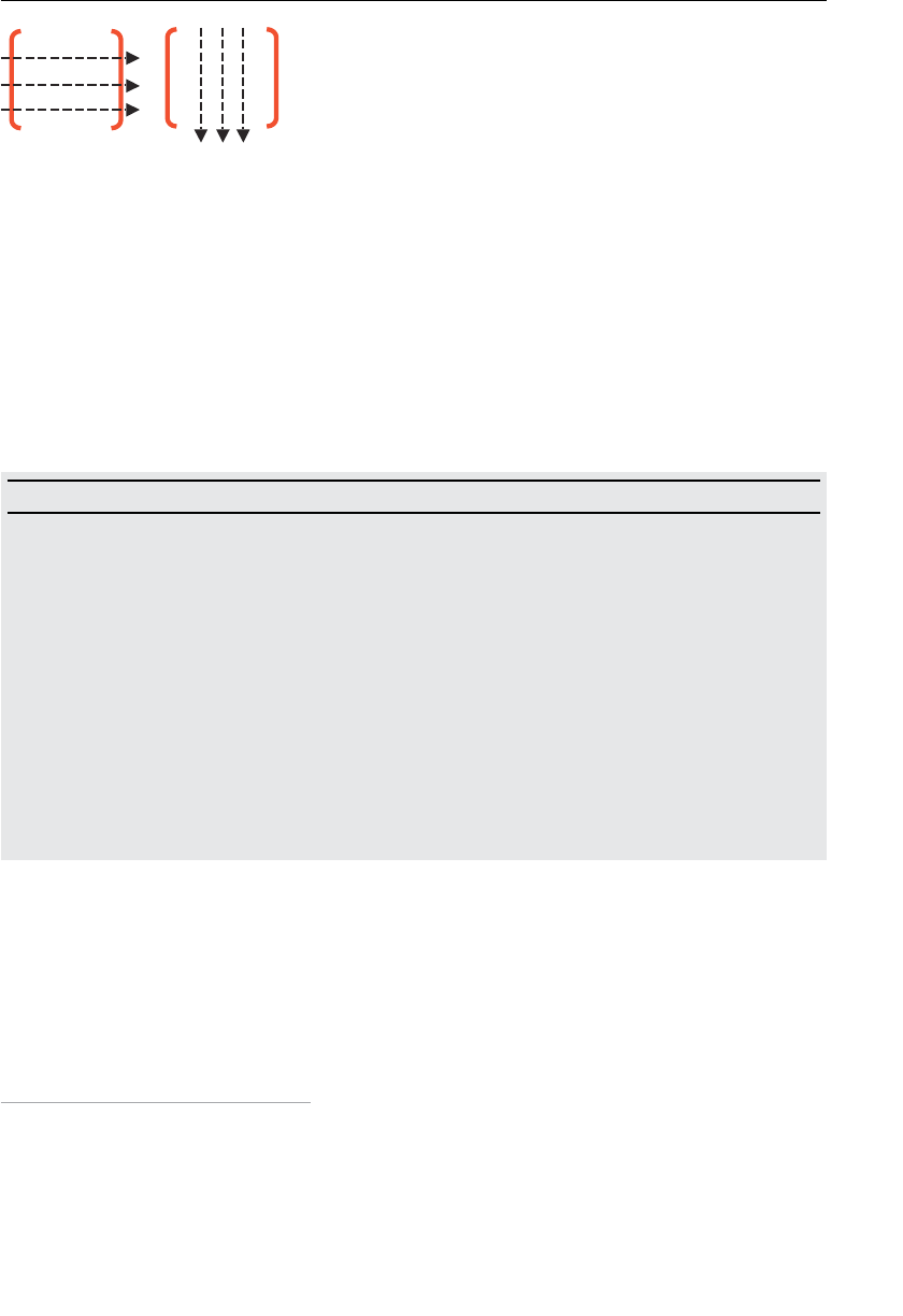
ptg11539634

CHAPTER 3 Drawing and Transforming Triangles

110

d c b a

h g f e

l k j i

p o n m

d c b a

h g f e

l k j i

p o n m

rojamnmulocrojamwor

Figure 3.27 Row major order and column major order

WebGL, just like OpenGL, requires you to store the elements of a matrix in the elements

of an array in column major order. So, for example, the matrix shown in Figure 3.27

is stored in an array as follows: [ a, e, i, m, b, f, j, n, c, g, k, o, d, h, l, p ]. In the sample

program, the rotation matrix is stored in the

Float32Array in this order in lines 49 to 52.

The array created is then passed to the uniform variable u_xformMatrix by using

gl.uniformMatrix4fv() at line 61. Note that the last letter of this method name is v ,

which indicates that the method can pass multiple data values to the variable.

gl.uniformMatrix4fv (location, transpose, array)

Assign the 4×4 matrix specified by array to the uniform variable specified by location.

Parameters location Specifies the storage location of the uniform variable.

Transpose Must be

false in WebGL.

array Specifies an array containing a 4×4 matrix in column

major order (typed array).

Return value None

Errors INVALID_OPERATION There is no current program object.

INVALID_VALUE transpose is not

false, or the length of array is less

than 16.

If you load and run the sample program in your browser, you’ll see the rotated triangle.

Congratulations! You have successfully learned how to use a transformation matrix to

rotate a triangle.

3 This parameter speci es whether to transpose the matrix or not. The transpose operation, which

exchanges the column and row elements of the matrix (see Chapter 7 ), is not supported by WebGL’s

implementation of this method and must always be set to false .

ptg11539634

Moving, Rotating, and Scaling 111

Reusing the Same Approach for Translation

Now, as you have seen with Equations 3.10 and 3.11 , you can represent both a translation

and a rotation using the same type of 4×4 matrix. Both equations use the matrices in the

form

<new coordinates> = <transformation matrix> * <original coordinates> . This

is coded in the vertex shader as follows:

7 ‘ gl_Position = u_xformMatrix * a_Position;n’ +

This means that if you change the elements of the array xformMatrix from those of a

rotation matrix to those of a translation matrix, you will be able to apply the translation

matrix to the triangle to achieve the same result as shown earlier but which used an equa-

tion ( Figure 3.18 ).

To do that, change line 17 in

RotatedTriangle_Matrix.js using the translation distances

from the previous example:

17 varTx = 0.5, Ty = 0.5, Tz = 0.0;

You need to rewrite the code for creating the matrix, remembering that you need to store

the elements of the matrix in column major order. Let’s keep the same name for the array

variable,

xformMatrix , even though it’s now being used to hold a translation matrix,

because it reinforces the fact that we are using essentially the same code. Finally, you are

not using the variable

ANGLE , so lines 43 to 45 are commented out:

43 // Create a rotation matrix

44 // var radian = Math.PI * ANGLE / 180.0; // Convert to radians

45 // var cosB = Math.cos(radian), sinB = Math.sin(radian);

47 // Note: WebGL is column major order

48 var xformMatrix = new Float32Array([

49 1.0, 0.0, 0.0, 0.0,

50 0.0, 1.0, 0.0, 0.0,

51 0.0, 0.0, 1.0, 0.0,

52 Tx, Ty, Tz, 1.0

53 ]);

Once you’ve made the changes, run the modified program, and you will see the same

output as shown in Figure 3.18 . By using a transformation matrix, you can apply various

transformations using the same vertex shader. This is why the transformation matrix is

such a convenient and powerful tool for 3D graphics, and it’s why we’ve covered it in

detail in this chapter.

Transformation Matrix: Scaling

Finally , let’s define the transformation matrix for scaling using the same assumption that

the original point is

p and the point after scaling is p’ .

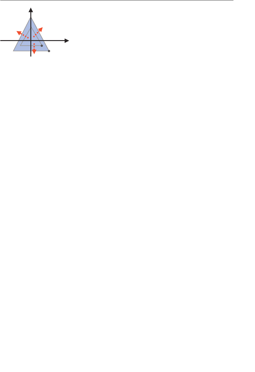
ptg11539634

CHAPTER 3 Drawing and Transforming Triangles

112

)‘z,‘y,‘x(‘p

)z,y,x(p

Figure 3.28 A scaling transformation

Assuming the scaling factor for the x-axis, y-axis, and z-axis is S

x , S

y , and S

z respectively,

you obtain the following equations:

x’ = S

x × x

y’ = S

y × y

z’ = S

z × z

The following transformation matrix can be obtained by comparing these equations with

Equation 3.9 .

⎡

⎣

⎢

⎤

⎦

⎥

⎡

⎣

⎢

⎤

⎦

⎥

⎡

⎣

⎢

⎤

⎦

⎥

‘

000

00 0

0001 1

As with the previous example, if you store this matrix in xformMatrix , you can scale the

triangle by using the same vertex shader you used in

RotatedTriangle_Matrix.js . For

example, the following sample program will scale the triangle by a factor of 1.5 in a verti-

cal direction, as shown in Figure 3.29 :

17 varSx = 1.0, Sy = 1.5, Sz = 1.0;

…

47 // Note: WebGL is column major order

48 var xformMatrix = new Float32Array([

49 Sx, 0.0, 0.0, 0.0,

50 0.0, Sy, 0.0, 0.0,

51 0.0, 0.0, Sz, 0.0,

52 0.0, 0.0, 0.0, 1.0

53 ]

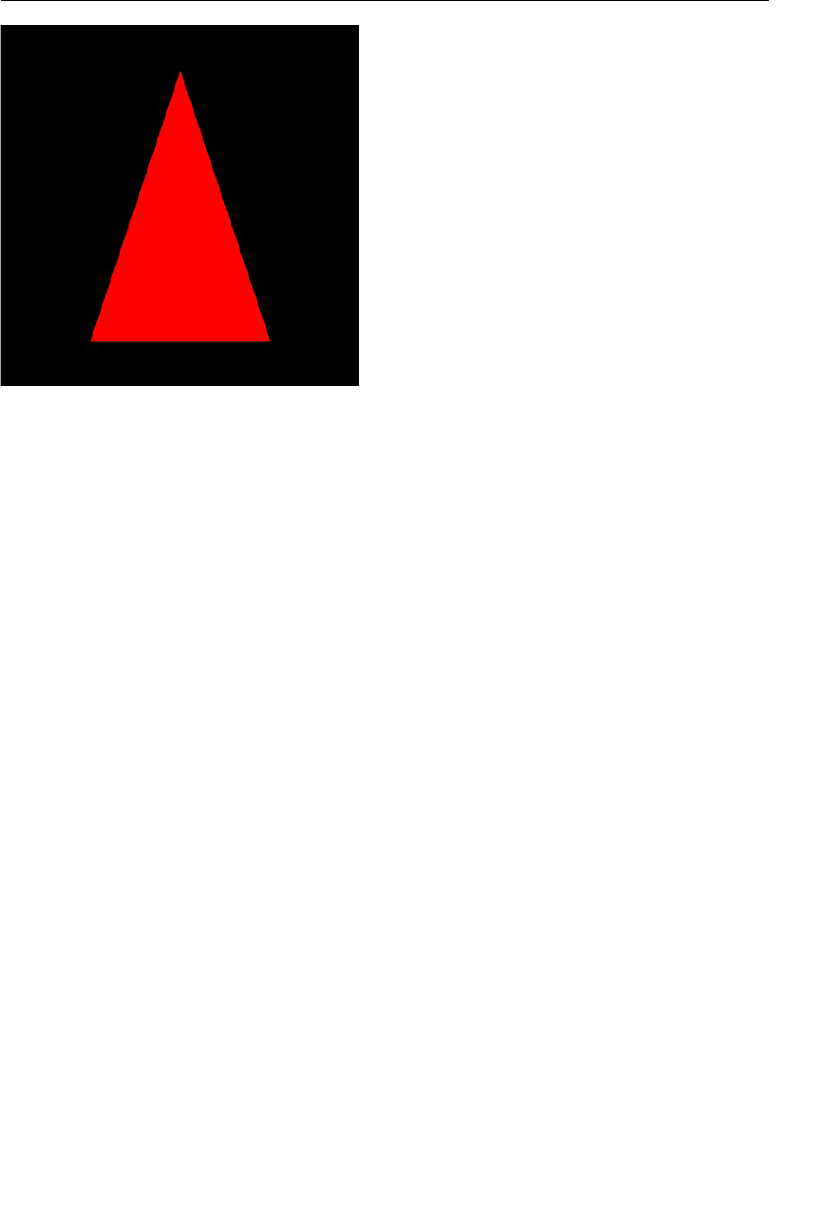
ptg11539634

Summary 113

Figure 3.29 Triangle scaled in a vertical direction

Note that if you specify 0.0 to

Sx , Sy , or Sz , the scaled size will be 0.0. If you want to keep

the original size, specify 1.0 as the scaling factor.

Summary

In this chapter, you explored the process of passing multiple items of information about

vertices to a vertex shader, the different types of shapes available to be drawn using that

information, and the process of transforming those shapes. The shapes dealt with in this

chapter changed from a point to a triangle, but the method of using shaders remained the

same, as in the examples in the previous chapter. You were also introduced to matrices

and learned how to use transformation matrices to apply translation, rotation, or scaling

to 2D shapes. Although it’s a little complicated, you should now have a good understand-

ing of the math behind calculating the individual transformation matrices.

In the next chapter, you’ll explore more complex transformations but will use a handy

library to hide the details, allowing you to focus on the higher-level tasks.

ptg11539634

This page intentionally left blank

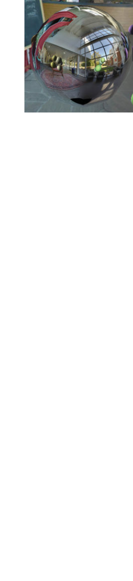
ptg11539634

Chapter 4

More Transformations and Basic Animation

Chapter 3 , “Drawing and Transforming Triangles,” explained how to use the buffer object to

draw more complex shapes and how to transform them using simple equations. Because this

approach is cumbersome for multiple transformations, you were then introduced to matrices and

their use to simplify transformation operations. In this chapter, you explore further transforma-

tions and begin to combine transformations into animations. In particular, you will

• Be introduced to a matrix transformation library that hides the mathematical details of

matrix operations

• Use the library to quickly and easily combine multiple transformations

• Explore animation and how the library helps you animate simple shapes

These techniques provide the basics to construct complex WebGL programs and will be used in

the sample programs in the following chapters.

Translate and Then Rotate

As you saw in Chapter 3 , although transformations such as translation, rotation, and scaling can

be represented as a 4×4 matrix, it is time consuming to specify each matrix by hand whenever

you write WebGL programs. To simply the task, most WebGL developers use a convenient library

that automates creating these matrices and hides the details. There are several public matrix

libraries for WebGL, but in this section, you’ll use a library created for this book and will see how

the library can be used to combine multiple transformations to achieve results such as “translate

and then rotate a triangle.”

ptg11539634

CHAPTER 4 More Transformations and Basic Animation

116

Transformation Matrix Library: cuon-matrix.js

In OpenGL , the parent specification of WebGL, there’s no need to specify by hand each

element of the transformation matrix when you use it. Instead, OpenGL supports a set

of handy functions that make it easy to construct the matrices. For example,

glTrans-

latef() , when called with translation distances for the x-, y-, and z-axes as arguments,

will create a translation matrix internally and then set up the matrix needed to translate a

shape (see Figure 4.1 ).

5001

08010

03100

1000

;)03,08,5(fetalsnarTlg

Figure 4.1 An example of glTranslatef() in OpenGL

Unfortunately, WebGL doesn’t provide these functions, so if you wanted to use this

approach you’d need to look for or write them yourself. Because these functions are

useful, we’ve created a JavaScript library for you,

cuon-matrix.js , which allows you to

create transformation matrices in a similar way to those specified in OpenGL. Although

this library was written specifically for this book, it is general purpose, and you are free to

use it in your own applications.

As you saw in Chapter 3 , JavaScript provides the sine and cosine function as methods of

the

Math object. In the same way, the functions for creating transformation matrices are

provided as methods of the

Matrix4 object defined in cuon-matrix.js .

Matrix4 is a new object, defined by the library, and as the name suggests, deals with 4×4

matrices. Internally, these are represented using a typed array,

Float32Array , which you

saw in Chapter 3 .

To get a feel for the library, let’s rewrite

RotatedTriangle_Matrix using the Matrix4 object

and its methods. The program for this example is called

RotatedTriangle_Matrix4 .

Because the Matrix4 object is defined in the library cuon-matrix.js , you need to load it

into your HTML file before using the object. To do this, you simply use the

<script> tag,

as shown in Listing 4.1 .

Listing 4.1 RotatedTriangle_Matrix4.html (The Codes for Loading the Library)

13 <script src=»../lib/webgl-debug.js»></script>

14 <script src=»../lib/cuon-utils.js»></script>

15 <script src=»../lib/cuon-matrix.js»></script>

16 <script src=»RotatedTriangle_Matrix4.js»></script>

Once loaded, let’s examine how to use it by comparing the previous RotatedTriangle_

Matrix.js with RotatedTriangle_Matrix4.js , which uses the new Matrix4 object.

ptg11539634

Translate and Then Rotate 117

Sample Program (RotatedTriangle_Matrix4.js)

This sample program is almost the same as RotatedTriangle_Matrix.js used in Chapter

3 except for the new steps that create the transformation matrix and pass it to

u_xformMa-

trix in the vertex shader.

In RotatedTriangle_Matrix.js , you created the transformation matrix as follows:

1 // RotatedTriangle_Matrix.js

…

43 // Create a rotation matrix

44 var radian = Math.PI * ANGLE / 180.0; // Convert to radians

45 varcosB = Math.cos(radian), sinB = Math.sin(radian);

47 // Note: WebGL is column major order

48 var xformMatrix = new Float32Array([

49 cosB, sinB, 0.0, 0.0,

50 -sinB, cosB, 0.0, 0.0,

51 0.0, 0.0, 1.0, 0.0,

52 0.0, 0.0, 0.0, 1.0

53 ]);

…

61 gl.uniformMatrix4fv(u_xformMatrix, false, xformMatrix);

In this sample program, you need to rewrite this part using a Matrix4 object and utilize its

method

setRotate() to calculate a rotation matrix. The following code snippet shows the

rewritten part from

RotatedTriangle_Matrix4.js :

1 // RotatedTriangle_Matrix4.js

…

47 // Create Matrix4 object for a rotation matrix

48 var xformMatrix = new Matrix4();

49 // Set the rotation matrix to xformMatrix

50 xformMatrix.setRotate(ANGLE, 0, 0, 1);

…

56 // Pass the rotation matrix to the vertex shader

57 gl.uniformMatrix4fv(u_xformMatrix, false, xformMatrix.elements );

You can see that the basic processing flow to create a matrix (line 48 and 50) and then

pass it to the uniform variable is the same as in the previous sample. A

Matrix4 object is

created using the

new operator in the same way that an Array or Date object is created in

JavaScript. Line 48 creates the

Matrix4 object, and then line 50 uses setRotate() to calcu-

late the rotation matrix and write it to the

xformMatrix object.

The setRotate() method takes four parameters: a rotation angle (specified in degrees, not

radians) and the rotation axis around which the rotation will take place. The rotation axis,

specified by x, y, and z, and associated direction are defined by the line drawn from

ptg11539634

CHAPTER 4 More Transformations and Basic Animation

118

(0, 0, 0) to (x, y, z). As you will remember from Chapter 3 ( Figure 3.21 ), the angle is posi-

tive if the rotation is performed in the clockwise direction around the rotation axis. In this

example, because the rotation is performed around the z-axis, the axis is set to (0, 0, 1):

50 xformMatrix.setRotate(ANGLE, 0, 0, 1);

Similarly, for the x-axis, you can specify x = 1, y =0, and z = 0 and for the y-axis, x = 0,

y = 1, and z = 0. Once you have set up the rotation matrix in the variable

xformMatrix ,

all you need to do is to pass the matrix to the vertex shader using the same method

gl.

uniformMatrix4fv() as before. Note that you cannot pass a Matrix4 object directly as

the last argument of this method because a typed array is required for the parameter.

However, you can retrieve the elements of the

Matrix4 object as a typed array by using its

property

elements , which you can then pass as shown at line 57:

57 gl.uniformMatrix4fv(u_xformMatrix, false, xformMatrix.elements );

The Matrix4 object supports the methods and properties shown in Table 4.1 .

Table 4.1 The Methods and Properties Supported by Matrix4

Methods and Properties Description

Matrix4.setIdentity() Initialize a matrix (to the identity matrix

* ).

Matrix4.setTranslate(x, y,

Set

Matrix4 to the translation matrix, which translates x

units in the direction of the x-axis, y units in the direction of

the y-axis, and z units in the direction of the z-axis.

Matrix4.setRotate(angle,

x, y, z)

Set

Matrix4 to the rotation matrix, which rotates angle

degrees around the rotation axis ( x , y , z ). The ( x , y , z ) coor-

dinates do not need to be normalized . (See Chapter 8 ,

“Lighting Objects.”)

Matrix4.setScale(x, y, z) Set Matrix4 to the scaling matrix with scaling factors x , y ,

and z .

Matrix4.translate (x, y,

Multiply the matrix stored in

Matrix4 by the translation

matrix, which translates x units in the direction of the x-axis,

y units in the direction of the y-axis, and z units in the direc-

tion of the z-axis, storing the result back into

Matrix4 .

Matrix4.rotate(angle, x,

y, z)

Multiply the matrix stored in

Matrix4 by the rotation matrix,

which rotates angle degrees around the rotation axis ( x , y ,

z ), storing the results back into

Matrix4 . The ( x , y , z ) coor-

dinates do not need to be normalized. (See Chapter 8 .)

Matrix4.scale(x, y, z) Multiply the matrix stored in Matrix4 by the scaling matrix,

with scaling factors x , y , and z , storing the results back into

Matrix4 .

ptg11539634

Translate and Then Rotate 119

Methods and Properties Description

Matrix4.set(m) Set the matrix m to Matrix4 . m must be a Matrix4 object.

Matrix4.elements The typed array ( Float32Array ) containing the elements of

the matrix stored in

Matrix4 .

* The identity matrix is a matrix that behaves for matrix multiplication like the scalar value 1 does for

scalar multiplication. Multiplying by the identity matrix has no effect on the other matrix. The identity

matrix has 1.0 in its diagonal elements.

As can be seen from the table, there are two types of methods supported by Matrix4 : those

whose names include

set , and those that don’t. The set methods calculate the transfor-

mation matrix using their parameters and then set or write the resulting matrix to the

Matrix4 object. In contrast, the methods without set multiply the matrix already stored

in the

Matrix4 object by the matrix calculated using the parameters and then store the

result back in the

Matrix4 object.

As you can see from the table, these methods are both powerful and flexible. More impor-

tantly, it makes it easy to quickly change transformations. For example, if you wanted to

translate the triangle instead of rotating, you could just rewrite line 50 as follows:

50 xformMatrix.setTranslate( 0.5, 0.5, 0.0);

The example uses the variable name xformMatrix to represent a generic transformation.

Obviously, you can use an appropriate variable name for the transformations within your

applications (such as

rotMatrix , as was used in Chapter 3 ).

Combining Multiple Transformation

Now that you are familiar with the basics of the Matrix4 object, let’s see how it can be

used to combine two transformations: a translation followed by a rotation. The sample

program

RotatedTranslatedTriangle does just that, resulting in Figure 4.2 . Note that

the example uses a smaller triangle so that you can easily understand the effect of the

transformation.

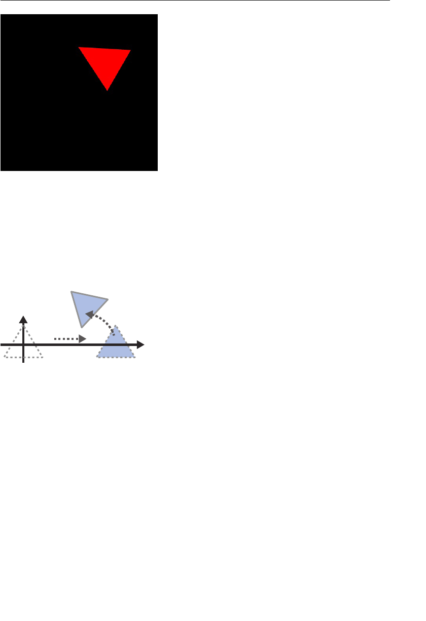
ptg11539634

CHAPTER 4 More Transformations and Basic Animation

120

Figure 4.2 RotatedTranslatedTriangle

Obviously, this example consists of the following two transformations, shown in

Figure 4.3:

1. Translate the triangle along the x-axis.

2. Rotate the triangle translated by (1).

)1(

)2(

Figure 4.3 The triangle translated and then rotated

Based on the explanations so far, we can write the equation of the translated triangle from

(1) as follows:

Equation 4.1

〈〉=

〈〉×〈〉

translated coordinates

translation matrix original coordinates

«»

Then you just need to rotate the

<>translated coordinates«» as follows:

Equation 4.2

〈〉=

〈〉×〈〉

translated and then rotated coordinates

rotation matrix translated coordinates

» «

ptg11539634

Translate and Then Rotate 121

You can calculate these equations separately, but they can be combined by substituting

Equation 4.1 into Equation 4.2 .

Equation 4.3

()

〈〉=

〈〉×〈〉×〈〉

translated and then rotated coordinates

rotation matrix translation matrix original coordinates

”  ”



Where

()

〈〉×〈〉×〈〉rotation matrix translation matrix original coordinates

is equal to

()

〈〉×〈〉×〈〉rotation matrix translation matrix original coordinates

This final step, calculating 〈〉×〈〉rotation matrix translation matrix

, can be carried out in a

JavaScript program and the result passed to the vertex shader. The combination of multi-

ple transformations like this is called model transformation (or modeling transforma-

tion ), and the matrix that performs model transformation is called the model matrix .

As a refresher, let’s just look at the multiplication of matrices, which is defined as follows:

⎡

⎢

⎤

⎥

⎡

⎢

⎤

⎥

aaa

bbb

00 01 02

10 11 12

20 21 22

00 01 02

10 11 12

20 21 22

Assuming two 3×3 matrices, A and B as shown, the product of A and B is defined as

follows:

Equation 4.4

×+×+× ×+×+× ×+×+×

×+×+ × ×+×+× ×+×+×

⎡

⎣

⎢

⎤

⎦

⎥

ababababababababab

ababab ababab ababab

ababababababababab

00 00 01 10 02 20 00 01 01 11 02 21 00 02 01 12 02 22

10 00 11 10 12 20 10 01 11 11 12 21 10 02 11 12 12 22

20 00 21 10 22 20 20 01 21 11 22 21 20 02 21 12 22 22

We use 3×3 matrices in the example, but the approach scales to the more usual 4×4 matri-

ces. However, note that the multiplication order of matrices is important. The result of

A * B is not equal to that of B * A.

As you would expect,

cuon-matrix.js supports a method to carry out matrix multiplica-

tion on

Matrix4 objects. Let’s look at how to use that method to combine two matrices to

support a translation followed by a rotation.

Sample Program (RotatedTranslatedTriangle.js)

Listing 4.2 shows RotatedTranslatedTriangle.js . The vertex shader and fragment shader

are the same as in

RotatedTriangle_Matrix4.js in the previous section except that the

name of the uniform variable is changed from

u_xformMatrix to u_ModelMatrix .

ptg11539634

CHAPTER 4 More Transformations and Basic Animation

122

Listing 4.2 RotatedTranslatedTriangle.js

1 // RotatedTranslatedTriangle.js

2 // Vertex shader program

3 var VSHADER_SOURCE =

4 ‘attribute vec4 a_Position;n’ +

5 ‘uniform mat4 u_ModelMatrix;n’ +

6 ‘void main() {n’ +

7 ‘ gl_Position = u_ModelMatrix * a_Position;n’ +

8 ‘}n’;

9 // Fragment shader program

…

16 function main() {

…

33 // Set the positions of vertices

34 var n = initVertexBuffers(gl);

…

40 // Create Matrix4 object for model transformation

41 var modelMatrix = new Matrix4();

43 // Calculate a model matrix

44 var ANGLE = 60.0; // Rotation angle

45 varTx = 0.5; // Translation distance

46 modelMatrix.setRotate(ANGLE, 0, 0, 1); // Set rotation matrix

47 modelMatrix.translate(Tx, 0, 0); // Multiply modelMatrix by the calculated

➥translation matrix

49 // Pass the model matrix to the vertex shader

50 var u_ModelMatrix = gl.getUniformLocation(gl.program, ‘ u_ModelMatrix’);

…

56 gl.uniformMatrix4fv(u_ModelMatrix, false, modelMatrix.elements);

…

63 // Draw a triangle

64 gl.drawArrays(gl.TRIANGLES, 0, n);

65 }

67 function initVertexBuffers(gl) {

68 var vertices = new Float32Array([

69 0.0, 0.3, -0.3, -0.3, 0.3, -0.3

70 ]);

71 var n = 3; // The number of vertices

…

99 return n;

100 }

ptg11539634

Translate and Then Rotate 123

The key lines in this listing are lines 46 and 47, which calculate

<>×< >rotation matrix translation matrix

46 modelMatrix.setRotate(ANGLE, 0, 0, 1); // Set rotation matrix

47 modelMatrix.translate(Tx, 0, 0); // Multiply modelMatrix by the calculated

➥translation matrix

Because line 46 uses a method with set ( setRotate()) , the rotation matrix that is calcu-

lated using the parameters is written to the variable

modelMatrix . The next line, 47,

uses a method without

set ( translate()) , which, as explained earlier, calculates the

translation matrix using the parameters and then multiplies the matrix in

modelMa-

trix by the newly calculated translation matrix and writes the result back into model-

Matrix . So, if modelMatrix already contains a rotation matrix, this method calculates

〈〉×〈〉rotation matrix translation matrix

and stores the result back into

modelMatrix .

You may have noticed that the order of “translate first and then rotate” is the opposite of

the order of the matrices in the calculation 〈〉×〈〉rotation matrix translation matrix

. As shown in

Equation 4.3 , this is because the transformation matrix is multiplied by the original vertex

coordinates of the triangle.

The result of this calculation is passed to

u_ModelMatrix in the vertex shader at line

56, and then the drawing operation (line 64) is the same as usual. If you now load this

program into your browser, you can see a red triangle, which has been translated and then

rotated.

Experimenting with the Sample Program

Let’s rewrite the sample program to first rotate the triangle and then translate it. This

simply requires you to exchange the order of the rotation and translation. In this

case, you should note that the translation is performed first by using the

set method,

setTranslate() :

46 modelMatrix.setTranslate(Tx, 0, 0);

47 modelMatrix.rotate(ANGLE, 0, 0, 1);

Figure 4.4 shows this sample program.

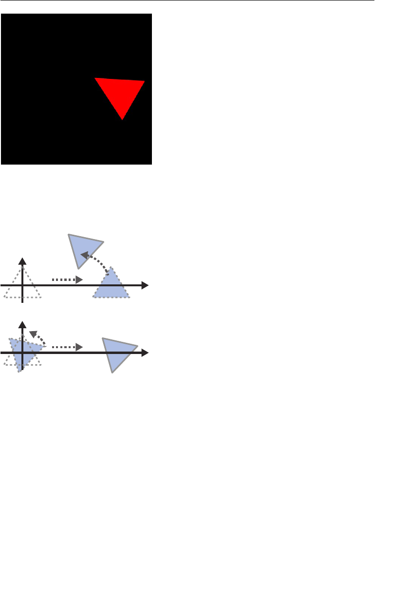
ptg11539634

CHAPTER 4 More Transformations and Basic Animation

124

Figure 4.4 A triangle “rotated first and then translated”

As you can see, by changing the order of a rotation and translation, you get a different

result. This becomes obvious when you examine Figure 4.5 .

etalsnartnehtdnatsrifetator

etatornehtdnatsrifetalsnart

)1(

)2(

y)1(

)2(

Figure 4.5 The order of transformations will show different results

That concludes the initial explanation of the use of methods defined in

cuon-matrix.js

to create transformation matrices. You’ll be using them throughout the rest of this book,

so you’ll have plenty of chance to study them further.

Animation

So far, this chapter has explained how to transform shapes and use the matrix library to

carry out transformation operations. You now have enough knowledge of WebGL to start

on the next step of applying this knowledge to animate shapes.

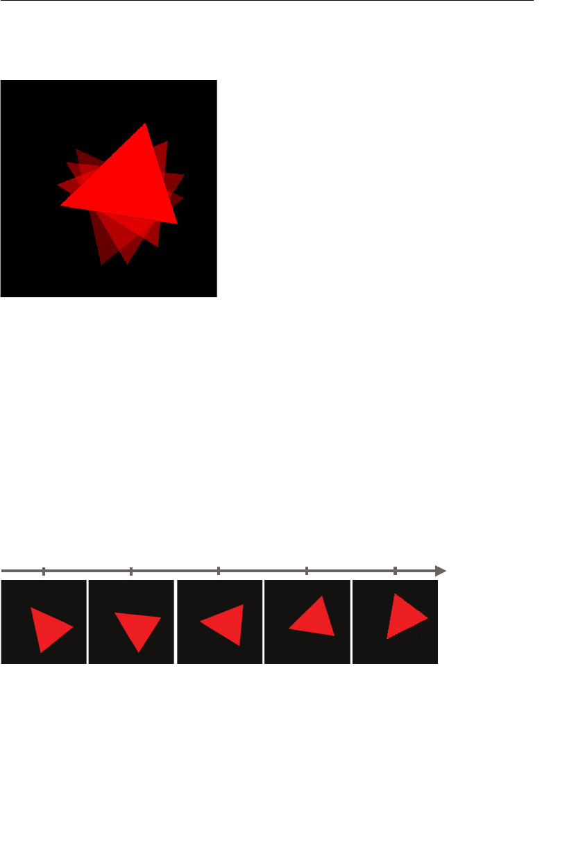
ptg11539634

Animation 125

Let’s start by constructing a sample program, RotatingTriangle , which continually rotates

a triangle at a constant rotation speed (45 degrees/second). Figure 4.6 shows multiple over-

laid screenshots of

RotatingTriangle so that you can see the rotation.

Figure 4.6 Multiple overlaid screenshots of RotatingTriangle

The Basics of Animation

To animate a rotating triangle, you simply need to redraw the triangle at a slightly differ-

ent angle each time it draws.

Figure 4.7 shows individual triangles that are drawn at times t0, t1, t2, t3, and t4. Each

triangle is a still image, but you can see that each has a slightly different rotation angle.

When you see a series of these triangles sequentially, your mind interpolates the changes

between them and then puts them together as a smooth flow of animation, just like a flip

book. Of course, you need to clear the previous triangle before drawing a new one. (This is

why you must call

gl.clear() before drawing something.) You can apply this animation

method to both 2D shapes and 3D objects.

e m i t

4 t 3 t 2 t 1 t

Figure 4.7 Draw a slightly different triangle for each drawing

ptg11539634

CHAPTER 4 More Transformations and Basic Animation

126

Achieving animation in this way requires two key mechanisms:

Mechanism 1: Repeatedly calls a function to draw a triangle at times t0, t1, t2, t3, and

so on.

Mechanism 2: Clears the previous triangle and then draws a new one with the specified

angle each time the function is called.

The second mechanism is just a simple application of the knowledge you’ve learned so far.

However, the first mechanism is new, so let’s take it step by step by examining the sample

program.

Sample Program (RotatingTriangle.js)

Listing 4.3 shows RotatingTriangle.js . The vertex shader and fragment shader are the

same as in the previous sample program. However, the vertex shader is listed to show the

multiplication of a matrix and vertex coordinates.

The following three points differ from the previous sample program:

• Because the program needs to draw a triangle repeatedly, it’s been modified to

specify the clear color at line 44, not just before the drawing operation. Remember,

the color stays in the WebGL system until it’s overwritten.

• The actual mechanism [Mechanism 1] to repeatedly call a drawing function has been

added (lines 59 to 64).

• [Mechanism 2] The operations to clear and draw a triangle were defined as a func-

tion (

draw() at line 102).

These differences are highlighted in Listing 4.3 (lines 1 to 3). Let’s look at them in more

detail.

Listing 4.3 RotatingTriangle.js

1 // RotatingTriangle.js

2 // Vertex shader program

3 var VSHADER_SOURCE =

4 ‘attribute vec4 a_Position;n’ +

5 ‘uniform mat4 u_ModelMatrix;n’ +

6 ‘void main() {n’ +

7 ‘ gl_Position = u_ModelMatrix * a_Position;n’ +

8 ‘}n’;

9 // Fragment shader program

…

16 // Rotation angle (degrees/second)

17 var ANGLE_STEP = 45.0;

ptg11539634

Animation 127

19 function main() {

…

36 // Set the positions of vertices

37 var n = initVertexBuffers(gl);

…

43 // Set the color for clearing <canvas> <- (1)

44 gl.clearColor(0.0, 0.0, 0.0, 1.0);

46 // Get the storage location of u_ModelMatrix variable

47 var u_ModelMatrix = gl.getUniformLocation(gl.program, ‘ u_ModelMatrix’);

…

53 // Current rotation angle of a triangle

54 varcurrentAngle = 0.0;

55 // Matrix4 object for model transformation

56 var modelMatrix = new Matrix4();

58 // Start to draw a triangle <- (2)

59 var tick = function() {

60 currentAngle = animate(currentAngle);// Update the rotation angle

61 draw(gl, n, currentAngle, modelMatrix, u_ModelMatrix);

62 requestAnimationFrame(tick);// Request that the browser calls tick

63 };

64 tick();

65 }

67 function initVertexBuffers(gl) {

68 var vertices = new Float32Array ([

69 0.0, 0.5, -0.5, -0.5, 0.5, -0.5

70 ]);

71 var n = 3; // The number of vertices

…

96 return n;

97 }

99 function draw(gl,n, currentAngle, modelMatrix, u_ModelMatrix){ <-(3)

100 // Set up rotation matrix

101 modelMatrix.setRotate(currentAngle, 0, 0, 1);

102

103 // Pass the rotation matrix to the vertex shader

104 gl.uniformMatrix4fv( u_ModelMatrix, false, modelMatrix.elements);

105

106 // Clear <canvas>

107 gl.clear(gl.COLOR_BUFFER_BIT);

108

109 // Draw a triangle

ptg11539634

CHAPTER 4 More Transformations and Basic Animation

128

110 gl.drawArrays(gl.TRIANGLES, 0, n);

111 }

112

113 // Last time when this function was called

114 var g_last = Date.now();

115 function animate(angle) {

116 // Calculate the elapsed time

117 v ar now = Date.now();

118 var elapsed = now — g_last; // milliseconds

119 g_last = now;

120 // Update the current rotation angle (adjusted by the elapsed time)

121 var newAngle = angle + (ANGLE_STEP * elapsed) / 1000.0;

122 return newAngle %= 360;

126 }

Line 7 in the vertex shader is just a multiplication of a matrix and the vertex coordinates

in the same way as

RotatedTranslatedTriangle.js ). u_ModelMatrix is a uniform variable,

and the rotation matrix is passed to the variable from a JavaScript program:

7 ‘ gl_Position = u_ModelMatrix * a_Position;n’ +

The variable ANGLE_STEP at line 17 defines the rotation angles per second and is set to 45

degrees/second:

17 var ANGLE_STEP = 45.0;

The main() function starts from line 19, but because the code from lines 19 to 37, which

specifies the vertex coordinates, is the same as before, it is omitted.

The first of the three differences is that you specify the clear color once only: at line 44.

Line 47 then retrieves the storage location of

u_ModelMatrix in the vertex shader. Because

this location never changes, it’s more efficient to do only this once:

47 var u_ModelMatrix = gl.getUniformLocation(gl.program, ‘u_ModelMatrix’);

The variable u_ModelMatrix is then used in the draw() function (line 99) that draws the

triangle.

The value of the variable

currentAngle starts at 0 degrees and stores how many degrees

the triangle should be rotated from its original position each time it is drawn. As in the

simple rotation examples earlier, it calculates the rotation matrix needed for the trans-

formation. The variable

modelMatrix defined at line 56 is a Matrix4 object used to hold

the rotation matrix in

draw() . This matrix could be created within draw() ; however, that

would require a new

Matrix4 object to be created each time draw() is called, which would

be inefficient. For this reason, the object is created at line 56 and then passed to

draw() at

line 61.

ptg11539634

Animation 129

Lines 59 to 64 implement Mechanism 1 as the function tick , which is repeatedly called

to draw the triangle. Before you look at how the overall “tick” mechanism actually works,

let’s look at what happens each time it is called:

53 // Current rotation angle of a triangle

54 varcurrentAngle = 0.0;

55 // Matix4 object for model transformation

56 var modelMatrix = new Matrix4();

58 // Start to draw a triangle <- (2)

59 var tick = function() {

60 currentAngle = animate(currentAngle); // Update the rotation angle

61 draw(gl, n, currentAngle, modelMatrix, u_ModelMatrix);

62 requestAnimationFrame(tick); // Request that the browser callstick

63 };

64 tick();

Within tick , the call to the function animate() at line 60 updates the current rotation

angle of the triangle, and then the call to

draw() at line 61 draws a triangle using gl.

drawArrays() .

draw() is passed the rotation matrix, which rotates the triangle to currentAngle degrees.

In turn, it passes the matrix to the

u_ModelMatrix variable in the vertex shader before

calling

gl.drawArrays() (lines 104 to 110). This code appears quite complex, so let’s

examine each part in turn.

Repeatedly Call the Drawing Function (tick())

As described earlier, to animate the triangle, you need to perform the following two steps

repeatedly: (1) update the current rotation angle of a triangle (

currentAngle ), and then (2)

call the drawing function with the angle to draw the triangle. Lines 59 to 64 implement

these processing steps.

In this sample program, these tasks are defined by the three operations of line 60, 61,

and 62. These operations are grouped in a single anonymous function using

function() ,

and the function is assigned to the variable

tick (see Figure 4.8 ). You use an anonymous

function if you want to pass the local variables defined in

main() ( gl , n , currentAngle ,

modelMatrix , and u_ModelMatrix ) to draw() as arguments when draw() is called at line 61.

If you need a refresher on anonymous functions, refer to Chapter 2 , “Your First Step with

WebGL,” where you used one to register an event handler.

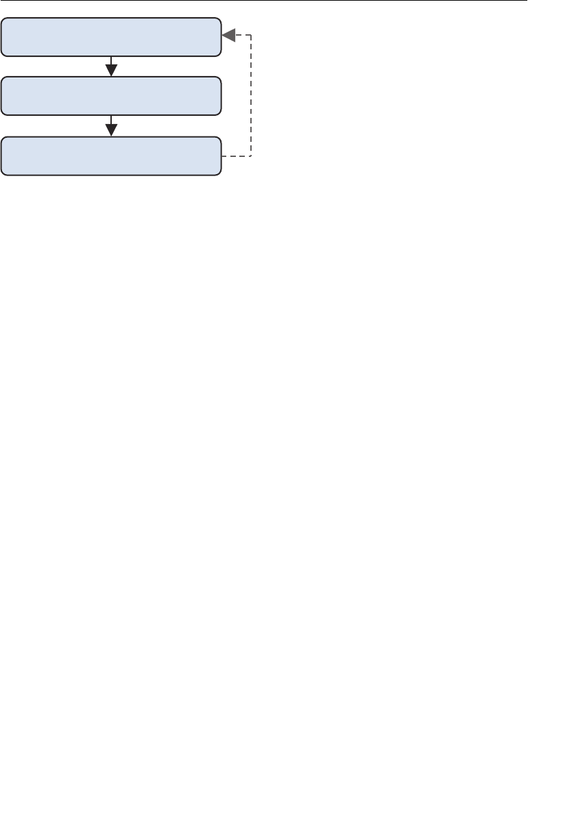
ptg11539634

CHAPTER 4 More Transformations and Basic Animation

130

elgnanoitatortnerrucehtetadpU

)06enil(

elgnaehtgnisuelgnairtawarD

)16enil(

noitcnufsihtsllacresworbehttahttseuqeR

)26enil(niaga))(kcit(

Figure 4.8 The operations assigned to “tick”

You can use this basic approach for all types of animation. It is a key technique in 3D

graphics.

When you call

requestAnimationFrame() at line 62, you are requesting the browser to call

the function specified as the first parameter at some future time when the three opera-

tions assigned to

tick will be executed again. You’ll look at requestAnimationFrame() in a

moment. For now, let’s finish examining the operations executed in

tick() .

Draw a Triangle with the Specified Rotation Angle (draw())

The draw() function takes the following five parameters:

• gl: The context in which to draw the triangle

• n: The number of vertices

• currentAngle: The current rotation angle

• modelMatrix: A Matrix4 object to store the rotation matrix calculated using curren-

tAngle

• u_ModelMatrix: The location of the uniform variable to which the modelMatrix is

passed

The actual function code is found in lines 99 to 111:

99 function draw(gl, n, currentAngle, modelMatrix, u_ModelMatrix) {

100 // Set the rotation matrix

101 modelMatrix.setRotate(currentAngle, 0, 0, 1);

102

103 // Pass the rotation matrix to the vertex shader

104 gl.uniformMatrix4fv( u_ModelMatrix, false, modelMatrix.elements);

105

106 // Clear <canvas>

107 gl.clear(gl.COLOR_BUFFER_BIT);

ptg11539634

Animation 131

108

109 // Draw the triangle

110 gl.drawArrays(gl.TRIANGLES, 0, n);

111 }

First, line 101 calculates the rotation matrix using the setRotate() method provided by

cuon-matrix.js , writing the resulting matrix to modelMatrix :

101 modelMatrix.setRotate(currentAngle, 0, 0, 1);

Next, line 104 passes the matrix to the vertex shader by using gl.uniformMatrix4fv() :

104 gl.uniformMatrix4fv(u_ModelMatrix, false, modelMatrix.elements);

After that, line 107 clears the <canvas> and then calls gl.drawArrays() at line 110 to

execute the vertex shader to actually draw the triangle. Those steps are the same as used

before.

Now let’s return to the third operation,

requestAnimationFrame() , which requests the

browser to call the function

tick() at some future time.

Request to Be Called Again (requestAnimationFrame())

Traditionally, if you wanted to repeatedly execute specific tasks (functions) in JavaScript,

you used the method

setInterval() .

setInterval (func, delay)

Call the function specified by func multiple times with intervals specified by delay.

Parameters func Specifies the function to be called multiple times.

delay Specifies the intervals (in milliseconds).

Return value Timer id

However, because this JavaScript method was designed before browsers started to support

multiple tabs, it executes regardless of which tab is active. This can lead to performance

problems, so a new method,

requestAnimationFrame() , was recently introduced. The

function scheduled using this method is only called when the tab in which it was defined

is active. Because

requestAnimationFrame() is a new method and not yet standardized,

it is defined in the library supplied by Google,

webgl-utils.js , which handles the differ-

ences among different browsers.

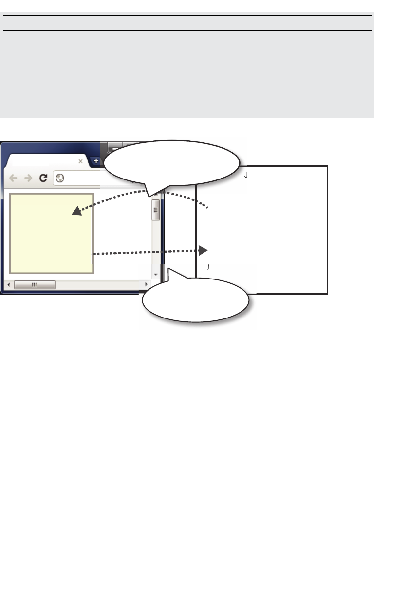
ptg11539634

CHAPTER 4 More Transformations and Basic Animation

132

requestAnimationFrame (func)

Requests the function specified by func to be called on redraw (see Figure 4.9 ). This

request needs to be remade after each callback.

Parameters func Specifies the function to be called later. The function takes a

“time” parameter, indicating the timestamp of the callback.

Return value Request id

…

;)kcit(emarFnoitaminAtseuqer

…

{)(kcitnoitcnuf

…

r e s w o r b e h t n e h W

, n e e r c s e h t s w a r d e r

s l l a c r e s w o r b e h t

. ) ( k c i t

t p i r c S a v a J

s a v n a c

}

l l a c o t r e s w o r b e h t t s e u q e R

r e s w o r b e h t n e h w ) ( k c i t

. n e e r c s e h t s w a r d e r

Figure 4.9 The requestAnimationFrame () mechanism

By using this method, you avoid animation in inactive tabs and do not increase the load

on the browser. Note, you cannot specify an interval before the function is called; rather,

func (the first parameter) will be called when the browser wants the web page contain-

ing the element (the second parameter) to be painted. In addition, after calling the func-

tion, you need to request the callback again because the previous request is automatically

removed once it’s fulfilled. Line 62 makes that request again once

tick is called and

makes it possible to call

tick() repeatedly:

62 requestAnimationFrame(tick); // Request the browser to call tick

If you want to cancel the request to call the function, you need to use

cancelAnimationFrame() .

ptg11539634

Animation 133

cancelAnimationFrame (requestID)

Cancel the function registered by

requestAnimationFrame() .

Parameter requestID Specifies the return value of

requestAnimationFrame() .

Return value None

Update the Rotation Angle (animate())

Finally, let’s see how to update the current rotation angle. The program maintains the

current rotation angle of the triangle (that is, how many degrees the triangle has been

rotated from its original position) in the variable

currentAngle (defined at line 54). It

calculates the next rotation angle based on this current value.

The update of

currentAngle is carried out in the function animate() , which is called at

line 60. This function, defined at line 115, takes one parameter,

angle , which represents

the current rotation angle and returns the new rotation angle:

60 currentAngle = animate(currentAngle);// Update the rotation angle

61 draw(gl, n, currentAngle, modelMatrix, u_ModelMatrix);

…

113 // Last time this function was called

114 var g_last = Date.getTime();

115 function animate(angle) {

116 // Calculate the elapsed time

117 var now = Date.getTime();

118 var elapsed = now — g_last;

119 g_last = now;

120 // Update the current rotation angle (adjusted by the elapsed time)

121 var newAngle = angle + (ANGLE_STEP * elapsed) / 1000.0;

122 return newAngle %= 360;

123 }

The process for updating the current rotation angle is slightly complicated. Let’s look at

the reason for that by using Figure 4.10 .

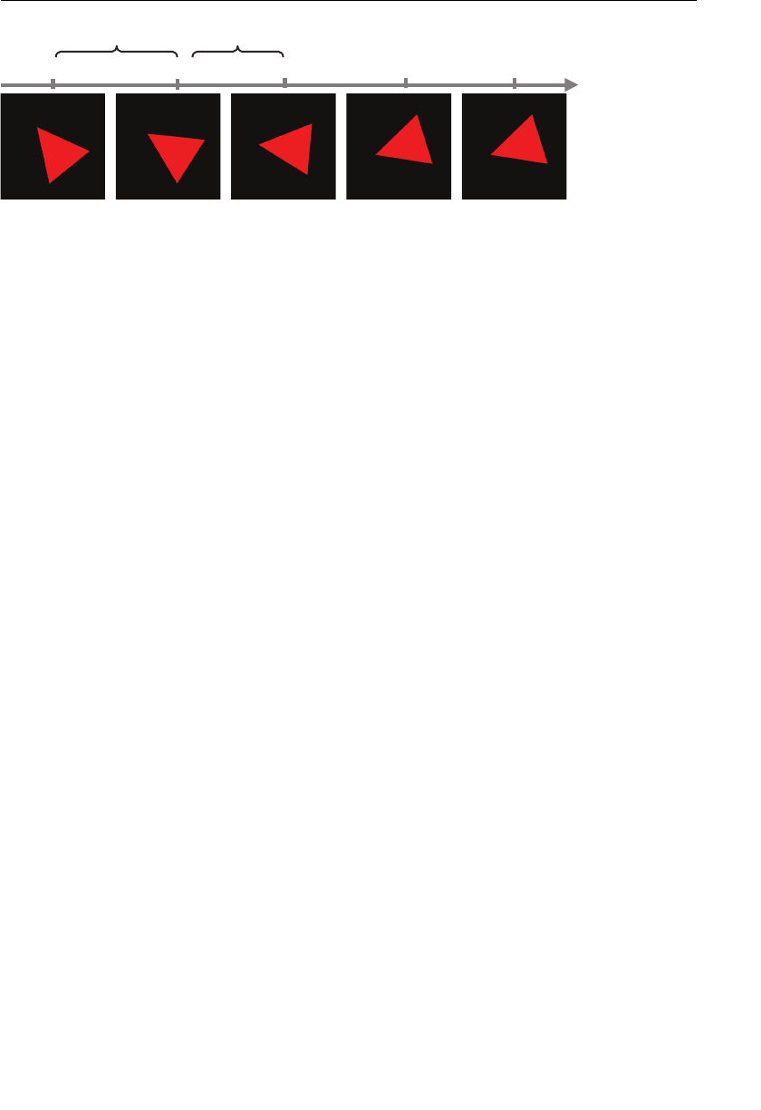
ptg11539634

CHAPTER 4 More Transformations and Basic Animation

134

emit

4t3t2t1t0t

0i i01i ot lauqe ton si 1 i

Figure 4.10 The interval times between each tick() vary

Figure 4.10 illustrates the following:

• tick() is called at t0. It calls draw() to draw the triangle and then reregisters tick() .

• tick() is called at t1. It calls draw() to draw the triangle and then reregisters tick() .

• tick() is called at t2. It calls draw() to draw the triangle and then reregisters tick() .

The problem here is that the interval times between t0 and t1, t1 and t2, and t2 and t3

may be different because of the load on the browser at that time. That is,

t1 – t0 could

be different from

t2 – t1 .

If the interval time is not constant, then simply adding a fixed amount of angle (degree/

second) to the current rotation angle each time

tick() is called will result in an apparent

acceleration or deceleration of the rotation speed.

For this reason, the function

animate() needs to be a little more sophisticated and must

determine the new rotation angle based on how long it has been since the function was

last called. To do that, you need to store the time that the function was last called into the

variable

g_last and store the current time into the variable now . Then you can calculate

how long it has been since the function was last called by subtraction and store the result

in the variable

elapsed (line 118). The amount of rotation is then calculated at line 121

using

elapsed as follows.

121 varnewAngle = angle + (ANGLE_STEP * elapsed) / 1000.0;

The variables g_last and now contain the return value from the method now() of a Date

object whose units are a millisecond (1/1000 second). Therefore, if you want to rotate

the triangle by

ANGLE_STEP (degree/second), you just need to multiply ANGLE_STEP by

elapsed /1000 to calculate the rotation angle. At line 121, you actually multiply ANGLE_

STEP by elapsed and then divide the result by 1000 because this is slightly more accurate,

but both have the same meaning.

Finally, line 122 ensures the value of

newAngle is less than 360 (degrees) and returns the

result.

ptg11539634

Animation 135

If you now load RotatedTriangle.html into your browser, you can check that the triangle

rotates at a constant speed. We will reuse this approach for animation in the following

chapters, so it’s worthwhile making sure you have mastered the details.

Experimenting with the Sample Program

In this section , let’s create an animation that consists of multiple transformations.

RotatingTranslatedTriangle translates a triangle 0.35 units in the positive direction of

the x-axis first and then rotates the triangle by 45 degrees/second.

This is easy to achieve if you remember that multiple transformations can be realized by

multiplying each transformation matrix together (refer to Chapter 3 ).

To do this, you just need to insert the translation at line 102. Because the variable

model-

Matrix already contains the rotation matrix, you can use translate() , rather than

setTranslate() , to multiply modelMatrix by the translation matrix:

99 function draw(gl, n, currentAngle, modelMatrix, u_ModelMatrix) {

100 // Set a rotation matrix

101 modelMatrix.setRotate(currentAngle, 0, 0, 1);

102 modelMatrix.translate(0.35, 0, 0);

103 // Pass the rotation matrix to the vertex shader

104 gl.uniformMatrix4fv( u_ModelMatrix, false, modelMatrix.elements);

If you load the example, you will see the animation shown in Figure 4.11 .

Figure 4.11 Multiple overlaid screenshots of RotatingTranslatedTriangle

Finally, for those of you wanting a little control, on the companion site for this book is

a sample program, named

RotatingTriangle_withButtons , that allows dynamic control

of the rotation speed using buttons (see Figure 4.12 ). You can see the buttons below the

<canvas> .

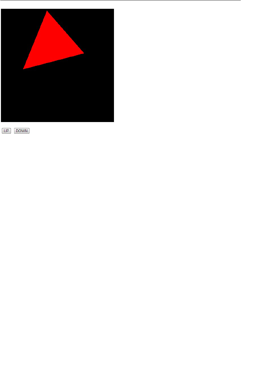
ptg11539634

CHAPTER 4 More Transformations and Basic Animation

136

Figure 4.12 RotatingTriangle_withButtons

Summary

This chapter explored the process of transforming shapes using the transformation matrix

library, combining multiple basic transformations to create a complex transformation, and

animating shapes using the library. There are two key lessons in this chapter: (1) Complex

transformations can be realized by multiplying a series of basic transformation matrices;

(2) You can animate shapes by repeating the transformation and drawing steps.

Chapter 5 , “Using Colors and Texture Images,” is the last chapter that covers basic tech-

niques. It explores colors and textures. Once you master those, you will have enough

knowledge to create your own basic WebGL programs and will be ready to begin exploring

some of the more advanced capabilities of WebGL.

ptg11539634

Chapter 5

Using Colors and Texture Images

The previous chapters explained the key concepts underlying the foundations of

WebGL through the use of examples based on 2D shapes. This approach has given you

a good understanding of how to deal with single color geometric shapes in WebGL.

Building on these basics, you now delve a little further into WebGL by exploring the

following three subjects:

• Passing other data such as color information to the vertex shader

• The conversion from a shape to fragments that takes place between the vertex

shader and the fragment shader, which is known as the rasterization process

• Mapping images (or textures) onto the surfaces of a shape or object

This is the final chapter that focuses on the key functionalities of WebGL. After reading

this chapter, you will understand the techniques and mechanism for using colors

and textures in WebGL and will have mastered enough WebGL to allow you to create

sophisticated 3D scenes.

Passing Other Types of Information to Vertex

Shaders

In the previous sample programs, a single buffer object was created first, the vertex

coordinates were stored in it, and then it was passed to the vertex shader. However,

beside coordinates, vertices involved in 3D graphics often need other types of infor-

mation such as color information or point size. For example, let us take a look at a

program you used in Chapter 3 , “Drawing and Transforming Triangles,” which draws

three points:

MultiPoint.js . In the shader, in addition to the vertex coordinates, you

provided the point size as extra information. However, the point size was a fixed value

and set in the shader rather than passed from outside:

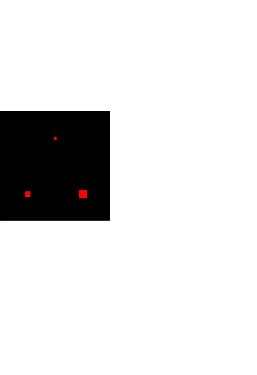
ptg11539634

CHAPTER 5 Using Colors and Texture Images

138

3 var VSHADER_SOURCE =

4 ‘attribute vec4 a_Position;n’ +

5 ‘void main() {n’ +

6 ‘ gl_Position = a_Position;n’ +

7 ‘ gl_PointSize = 10.0;n’ +

8 ‘}n’

Line 6 assigns the vertex coordinates to gl_Position , and line 7 assigns a fixed point

size of 10.0 to

gl_PointSize . If you now wanted to modify the size of that point from

your JavaScript program, you would need a way to pass the point size with the vertex

coordinates.

Let’s look at an example,

MultiAttributeSize , whose goal is to draw three points of

different sizes: 10.0, 20.0, and 30.0, respectively (see Figure 5.1 ).

Figure 5.1 MultiAttributeSize

In the previous chapter, you carried out the following steps to pass the vertex coordinates:

1. Create a buffer object.

2. Bind the buffer object to the target.

3. Write the coordinate data into the buffer object.

4. Assign the buffer object to the attribute variable.

5. Enable the assignment.

If you now wanted to pass several items of vertex information to the vertex shader

through buffer objects, you could just apply the same steps to all the items of information

associated with a vertex. Let’s look at a sample program that uses multiple buffers to do

just that.

ptg11539634

Passing Other Types of Information to Vertex Shaders 139

Sample Program (MultiAttributeSize.js)

MultiAttributeSize.js is shown in Listing 5.1 . The fragment shader is basically the same

as in

MultiPoint.js , so let’s omit it this time. The vertex shader is also similar, apart from

the fact that you add a new attribute variable that specifies the point size. The numbers 1

through 5 on the right of the listing note the five steps previously outlined.

Listing 5.1 MultiAttributeSize.js

1 // MultiAttributeSize.js

2 // Vertex shader program

3 var VSHADER_SOURCE =

4 ‘attribute vec4 a_Position;n’ +

5 ‘attribute float a_PointSize;n’ +

6 ‘void main() {n’ +

7 ‘ gl_Position = a_Position;n’ +

8 ‘ gl_PointSize = a_PointSize;n’ +

9 ‘}n’;

…

17 function main() {

…

34 // Set the vertex information

35 var n = initVertexBuffers(gl);

…

47 // Draw three points

48 gl.drawArrays(gl.POINTS, 0, n);

49 }

51 function initVertexBuffers(gl) {

52 var vertices = new Float32Array([

53 0.0, 0.5, -0.5, -0.5, 0.5, -0.5

54 ]);

55 var n = 3;

57 var sizes = new Float32Array([

58 10.0, 20.0, 30.0 // Point sizes

59 ]);

61 // Create a buffer object

62 var vertexBuffer = gl.createBuffer(); <-(1)

63 var sizeBuffer = gl.createBuffer(); <-(1′)

…

69 // Write vertex coordinates to the buffer object and enable it

70 gl.bindBuffer(gl.ARRAY_BUFFER, vertexBuffer); <-(2)

71 gl.bufferData(gl.ARRAY_BUFFER, vertices, gl.STATIC_DRAW); <-(3)

72 var a_Position = gl.getAttribLocation(gl.program, ‘a_Position’);

ptg11539634

CHAPTER 5 Using Colors and Texture Images

140

…

77 gl.vertexAttribPointer(a_Position, 2, gl.FLOAT, false, 0, 0); <-(4)

78 gl.enableVertexAttribArray(a_Position); <-(5)

80 // Write point sizes to the buffer object and enable it

81 gl.bindBuffer(gl.ARRAY_BUFFER, sizeBuffer); <-(2′)

82 gl.bufferData(gl.ARRAY_BUFFER, sizes, gl.STATIC_DRAW); <-(3′)

83 var a_PointSize = gl.getAttribLocation(gl.program, ‘a_PointSize’);

…

88 gl.vertexAttribPointer(a_PointSize, 1, gl.FLOAT, false, 0, 0); <-(4′)

89 gl.enableVertexAttribArray(a_PointSize); <-(5′)

…

94 return n;

95 }

First of all, let us examine the vertex shader in Listing 5.1 . As you can see, the attribute

variable

a_PointSize , which receives the point size from the JavaScript program, has been

added. This variable, declared at line 5 as a

float , is then assigned to gl_PointSize at line

8. No other changes are necessary for the vertex shader, but you will need a slight modi-

fication to the process in

initVertexBuffers() so it can handle several buffer objects. Let

us take a more detailed look at it.

Create Multiple Buffer Objects

The function initVertexBuffers() starts at line 51, and the vertex coordinates are

defined from lines 52 to 54. The point sizes are then specified at line 57 using the array

sizes :

57 var sizes = new Float32Array([

58 10.0, 20.0, 30.0 // Point sizes

59 ]);

A buffer object is created at line 62 for the vertex data, and at line 63 another buffer object

(

sizeBuffer ) is created for storing the array of “point sizes.”

From lines 70 to 78, the program binds the buffer object for the vertex coordinates, writes

the data, and finally assigns and enables the attribute variables associated with the buffer

object. These tasks are the same as those described in the previous sample programs.

Lines 80 to 89 are new additions for handling the different point sizes. However, the steps

are the same as for a vertex buffer. Bind the buffer object for the point sizes (

sizeBuffer )

to the target (line 81), write the data (line 82), assign the buffer object to the attribute

variable

a_PointSize (line 88), and enable it.

Once these steps in initVertexBuffers() are completed, the internal state of the WebGL

system looks like Figure 5.2 . You can see that the two separate buffer objects are created

and then assigned to the two separate attribute variables.

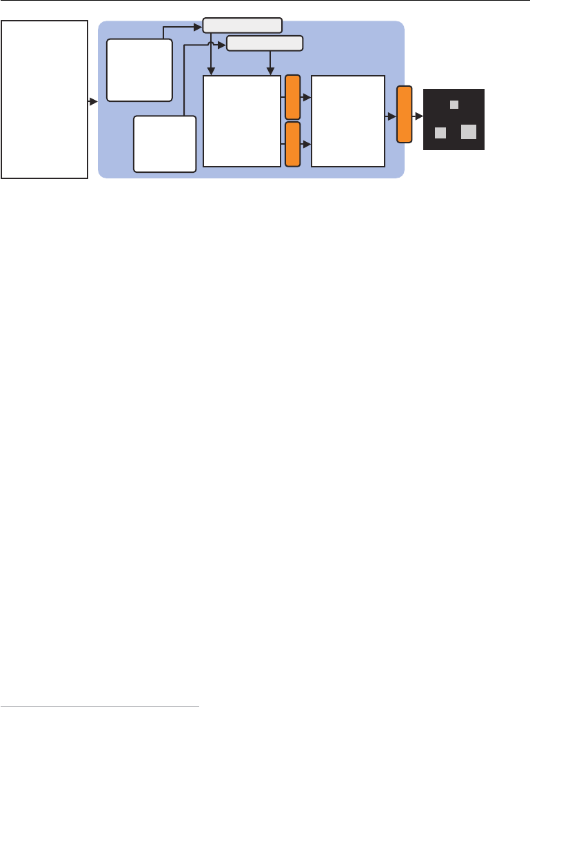
ptg11539634

Passing Other Types of Information to Vertex Shaders 141

gl_FragColor

{)(niamnoitcnuf

…LGbeWteg=lgrav

…

;)…(sredahStini

…

}

tnemgarF

redahS

gl_Position

redahSxetreV

noitisoP_aetubirtta

=roloCgarF_lg

;)…(4cev

=noitisoP_lg

;noitisoP_a

=eziStnioP_lg

;eziStnioP_a

ezIStnioP_aetu

birtta

tcejbOreffuB

5.0,0.0

5.0—,5.0—

5.0—,5.0

reffuBxetrev

reffuBezis

gl_PointSize

reffuBroloC

metsySLGbeW

,0.01

,0.02

0.03

tcejbOreffuB

tpircSavaJ

Figure 5.2 Using two buffer objects to pass data to a vertex shader

In this situation, when gl.drawArrays() at line 48 is executed, all the data stored inside

the buffer objects is sequentially passed to each attribute variable in the order it was stored

inside the buffer objects. By assigning this data to

gl_Position at line 7 and gl_PointSize

at line 8, respectively (the vertex shader’s program in Figure 5.2 ), you are now able to

draw different size objects located at different positions.

By creating a buffer object for each type of data in this way and then allocating it to the

attribute variables, you can pass several pieces of information about each vertex to the

vertex shader. Other types of information that can be passed include color, texture coordi-

nates (described in this chapter), and normals ( see Chapter 7 ), as well as point size.

The gl.vertexAttribPointer() Stride and Offset Parameters

Although multiple buffer objects are a great way to handle small amounts of data, in a

complicated 3D object with many thousands of vertices, you can imagine that managing

all the associated vertex data is an extremely difficult task. For example, imagine needing

to manually check each of these arrays when the total count of

MultiAttributeSize.js ’s

vertices and sizes reaches 1000.

1 However, WebGL allows the vertex coordinates and the

size to be bundled into a single component and provides mechanisms to access the differ-

ent data types. For example, you can group the vertex and size data in the following way

(refer to Listing 5.2 ), often referred to as interleaving .

Listing 5.2 An Array Containing Multiple Items of Vertex Information

var verticesSizes = new Float32Array([

// Vertex coordinates and size of a point

0.0, 0.5, 10.0, // The 1st point

-0.5, -0.5, 20.0, // The 2nd point

0.5, -0.5, 30.0 // The 3rd point

]);

1 I n practice, because modeling tools that create 3D models actually generate this data, there is no

necessity to either manually input them or visually check their consistency. The use of modeling

tools and the data they generate will be discussed in Chapter 10 .

ptg11539634

CHAPTER 5 Using Colors and Texture Images

142

As just described, once you have stored several types of information pertaining to the

vertex in a single buffer object, you need a mechanism to access these different data

elements. You can use the fifth ( stride ) and sixth ( offset ) arguments of

gl.vertexAttrib-

Pointer() to do this, as shown in the example that follows.

Sample Program (MultiAttributeSize_Interleaved.js)

Let’s construct a sample program, MultiAttributeSize_Interleaved , which passes multi-

ple data to the vertex shader, just like

MultiAttributeSize.js (refer to Listing 5.1 ), except

that it bundles the data into a single array or buffer. Listing 5.3 shows the program in

which the vertex shader and the fragment shader are the same as in

MultiAttributeSize.

js .

Listing 5.3 MultiAttributeSize_Interleaved.js

1 // MultiAttributeSize_Interleaved.js

2 // Vertex shader program

3 var VSHADER_SOURCE =

4 ‘attribute vec4 a_Position;n’ +

5 ‘attribute float a_PointSize;n’ +

6 ‘void main() {n’ +

7 ‘ gl_Position = a_Position;n’ +

8 ‘ gl_PointSize = a_PointSize;n’ +

9 ‘}n’;

…

17 function main() {

…

34 // Set vertex coordinates and point sizes

35 var n = initVertexBuffers(gl);

…

48 gl.drawArrays(gl.POINTS, 0, n);

49 }

51 function initVertexBuffers(gl) {

52 var verticesSizes = new Float32Array([

53 // Vertex coordinates and size of a point

54 0.0, 0.5, 10.0, // The 1st vertex

55 -0.5, -0.5, 20.0, // The 2nd vertex

56 0.5, -0.5, 30.0 // The 3rd vertex

57 ]);

58 var n = 3;

60 // Create a buffer object

61 var vertexSizeBuffer = gl.createBuffer();

…

ptg11539634

Passing Other Types of Information to Vertex Shaders 143

67 // Write vertex coords and point sizes to the buffer and enable it

68 gl.bindBuffer(gl.ARRAY_BUFFER, vertexSizeBuffer);

69 gl.bufferData(gl.ARRAY_BUFFER, verticesSizes, gl.STATIC_DRAW);

71 var FSIZE = verticesSizes.BYTES_PER_ELEMENT;

72 // Get the storage location of a_Position, allocate buffer, & enable

73 var a_Position = gl.getAttribLocation(gl.program, ‘a_Position’);

…

78 gl.vertexAttribPointer(a_Position, 2, gl.FLOAT, false, FSIZE * 3, 0);

79 gl.enableVertexAttribArray(a_Position); // Enable allocation

81 // Get the storage location of a_PointSize, allocate buffer, & enable

82 var a_PointSize = gl.getAttribLocation(gl.program, ‘a_PointSize’);

…

87 gl.vertexAttribPointer(a_PointSize, 1, gl.FLOAT, false, FSIZE * 3, FSIZE * 2);

88 gl.enableVertexAttribArray(a_PointSize); // Enable buffer allocation

…

93 return n;

94 }

The processing flow of the main() function in JavaScript is the same as

MultiAttributeSize.js , and only the initVertexBuffers() process is modified this time,

so let’s take a look at its content.

First, a typed array is defined at lines 52 to 57, as previously described in Listing 5.2 .

Following the usual processing steps, from line 61 to 69, a buffer object is created (line

61), the object is bound (line 68), and the data is written to the object (line 69). Next,

at line 71, the size (number of bytes) of the element in the

verticeSizes array is stored

in the variable

FSIZE , which will be needed later on. The size (number of bytes) of each

element of a typed array can be obtained through the property

BYTES_PER_ELEMENT .

From line 73 onward, you assign the buffer object to the attribute variable. Retrieving the

storage location of the attribute variable

a_Position at line 73 is similar to the previous

example, but the usage of the arguments of

gl.vertexAttribPointer() at line 78 is differ-

ent because the buffer now holds two types of data: vertex and point size.

You’ve already looked at the specification of

gl.vertexAttribPointer() in Chapter 3 , but

let’s take another look and focus on two parameters: stride and offset .

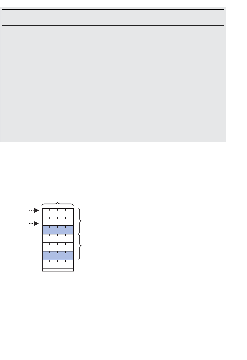
ptg11539634

CHAPTER 5 Using Colors and Texture Images

144

gl.vertexAttribPointer(location, size, type, normalized, stride,

offset)

Assign the buffer object bound to

gl.ARRAY_BUFFER to the attribute variable specified by

location . The type and format of the data written in the buffer is also specified.

Parameters location Specifies the storage location of the attribute variable.

size Specifies the number of components per vertex in the buffer

object (valid values are 1 to 4).

type Specifies the data format (in this case,

gl.FLOAT )

normalized

true or false . Used to indicate whether non- float data should

be normalized to [0, 1] or [–1, 1].

stride Specifies the stride length (in bytes) to get vertex data; that is,

the number of bytes between each vertex element

offset Specifies the offset (in bytes) in a buffer object to indicate where

the vertex data is stored from. If the data is stored from the

beginning. then offset is 0.

The stride specifies the number of bytes used by a group of related vertex data (in this

example, vertex coordinates and point size) inside the buffer object.

In previous examples, where you had only one type of information in the buffer—

vertices—you set the stride to 0. However, in this example, both vertices and point sizes

are laid out in the buffer, as shown in Figure 5.3 .

0.01

0.02

0.0

5.0

5.0—

5.0

TNEMELE_REP_SETYB.seziSsecitrev=EZISF

)3*EZISF(edirts

fotesffoehT

)0(noitisoP_a

fotesffoehT

eziStnioP_a

)2*EZISF(

)3*EZISF(edirts

NOTE : This figure is drawn assuming FSIZE=4

Figure 5.3 Stride and offset

As illustrated in Figure 5.3 , there are three components inside each group of vertex data

(two coordinates, one size), so you need to set the stride equal to three times the size of

each component in the group (that is, three times

FSIZE [the number of bytes per element

of the

Floats32Array ]).

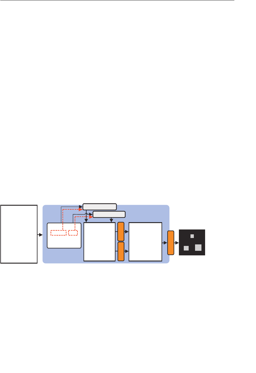
ptg11539634

Passing Other Types of Information to Vertex Shaders 145

The offset parameter indicates the distance to the first element that is being used for this

call. Because you are using the vertex coordinates that are positioned at the head of the

verticesSizes array, the offset is 0. So, at line 78, you specify them as the fifth ( stride ) and

sixth ( offset ) arguments of

gl.vertexAttribPointer() :

78 gl.vertexAttribPointer(a_Position, 2, gl.FLOAT, false, FSIZE * 3, 0);

79 gl.enableVertexAttribArray(a_Position); // Enable allocation

Finally, once the specification of the vertex coordinates has been set up, the assignment to

a_Position is enabled at line 79.

Next, from line 82, you need to do the same for the point size data, so assign a buffer

object to

a_PointSize . However, in this case, you are using the same buffer that you used

for vertex data, but you want different data from the buffer. You can make use of the sixth

argument offset to achieve this by setting the offset to the location at which the data (in

this case the point size) to be passed to

a_PointSize is positioned in the buffer. The first

two elements of the array are vertex coordinates, so the offset will accordingly be set to

FSIZE * 2 (refer to Figure 5.3 ). Line 87 shows both stride and offset set up correctly:

87 gl.vertexAttribPointer(a_PointSize, 1, gl.FLOAT, false, FSIZE * 3, FSIZE * 2);

88 gl.enableVertexAttribArray(a_PointSize); // Enable buffer allocation

The assignment to a_PointSize is enabled at line 88, and the only remaining task to

perform is the draw operation using

gl.drawArrays() .

Each time a vertex shader is invoked, WebGL will extract data from the buffer object using

the values specified in stride and offset and subsequently pass them to the attribute vari-

ables to be used for drawing (see Figure 5.4 ).

tpircSavaJ

{)(niamnoitcnuf

…LGbeWteg=lgrav

…

;)…(sredahStini

…

}

gl_Position

redahSxetreV

=noitisoP_lg

;noitisoP_a

=eziStnioP_lg

;eziStnioP_a

noitisoP_aetubirtta

eziStnioP_aetubirtta

gl_PointSize

gl_FragColor

reffuBroloC

,5.0,0.0,0.01

,5.0—,5.0-,0.02

,5.0—,5.0,0.03

tnemgarF

redahS

=roloCgarF_lg

;)(4cev

tcejbOreffuB

Figure 5.4 Internal behavior when stride and offset are used

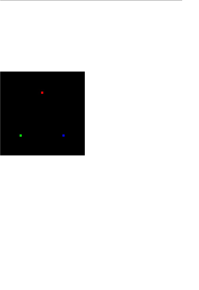
ptg11539634

CHAPTER 5 Using Colors and Texture Images

146

Modifying the Color (Varying Variable)

Now that you have seen how to pass several pieces of information to the vertex shader,

let’s use the technique to modify the color of each point. You can achieve this using the

procedure explained previously, substituting color information for point size in the buffer.

After storing the vertex coordinates and the color in the buffer object, you will assign the

color to the attribute variable, which handles the color.

Let’s construct a sample program,

MultiAttributeColor , that draws red, blue, and green

points. A screenshot is shown in Figure 5.5. (Because this book is black and white, it might

be difficult to appreciate the difference between the colors, so load and run the code in

your browser.)

Figure 5.5 MultiAttributeColor

As you may remember from Chapter 2 , “Your First Step with WebGL,” the fragment

shader actually handles attributes like color. Up until this point, you’ve set up color stati-

cally in the fragment shader code and not touched it again. However, although you have

learned how to pass the point color information to the vertex shader through the attri-

bute variable, the use of the

gl_FragColor variable, which sets the color information, is

restricted to the fragment shader. (Refer to the section “Fragment Shader” in Chapter 2 .)

Therefore, you need to find a way to communicate to the fragment shader the color infor-

mation previously passed to the vertex shader ( Figure 5.6 ).

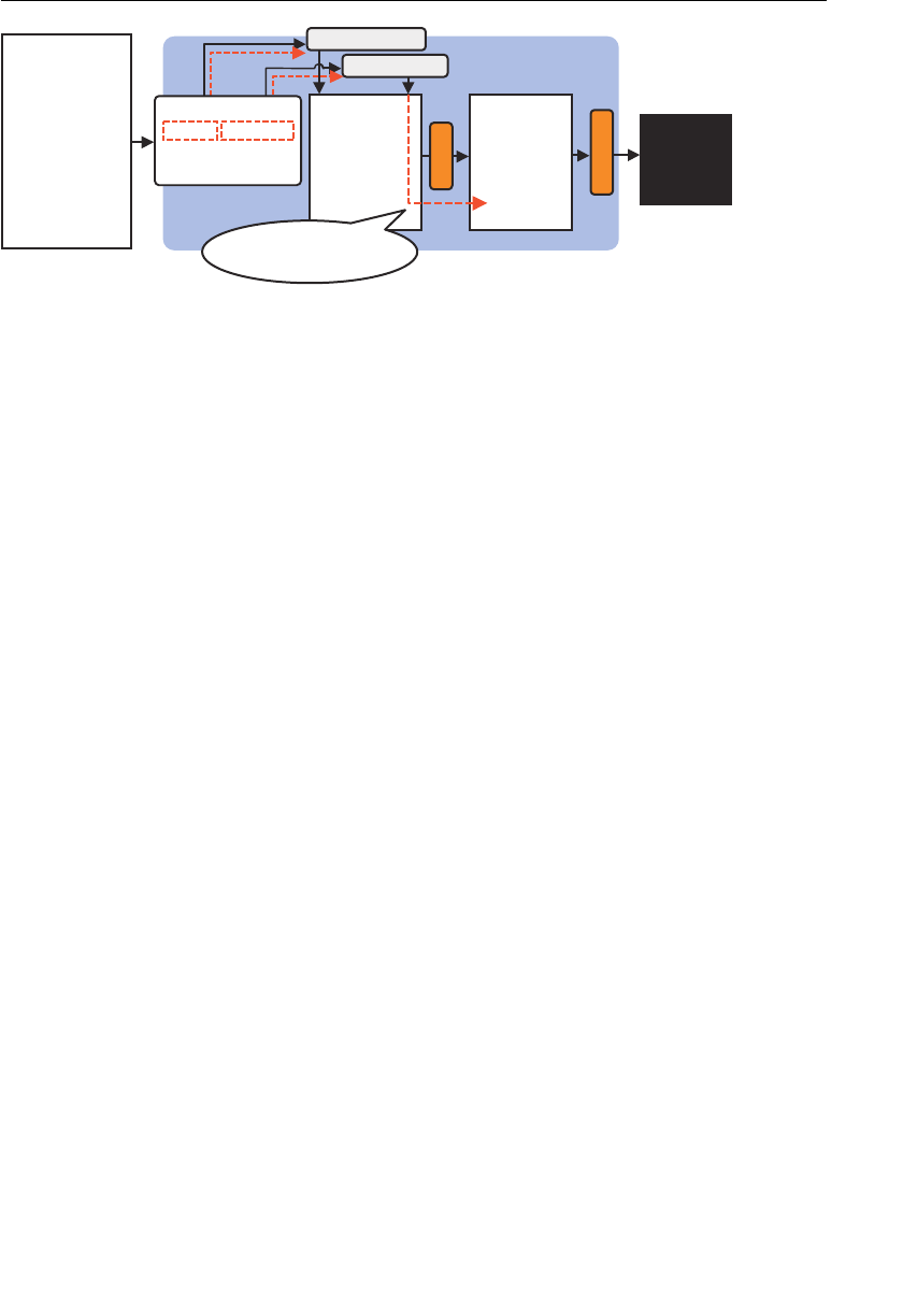
ptg11539634

Passing Other Types of Information to Vertex Shaders 147

gl_FragColor

{)(niamnoitcnuf

…LGbeWteg=lgrav

…

;)…(sredahStini

…

}

tnemgarF

redahS

gl_Position

roloCgarF_lg

=noitisoP_lg

;noitisoP_a

;noitisoP_aetubirtta

;roloC_aetubirtta

ewnacwoH

?atadssap

reffuBroloC

metsySLGbeW

,0.0,0.0,0.1,5.0,0.0

,0.0,0.1,0.0,5.0—,5.0—

0.1,0.0,0.0,5.0—,5.0

redahSxetreV

tcejbOreffuB

tpircSavaJ

Figure 5.6 Passing data from a vertex shader to a fragment shader

ColoredPoints ( Chapter 2 ), a uniform variable was used to pass the color informa-

tion to the fragment shader; however, because it is a “uniform” variable (not varying),

it cannot be used to pass different colors for each vertex. This is where a new method to

pass data to the fragment shader through the varying variable is needed and relies on a

mechanism that sends data from the vertex shader to the fragment shader: by using the

varying variable. Let’s look at a concrete sample program.

Sample Program (MultiAttributeColor.js)

Listing 5.4 shows the program, which looks similar to the program introduced in the

previous section,

MultiAttributeSize_Stride.js , but the part related to the vertex and

fragment shaders is actually slightly different.

Listing 5.4 MultiAttributeColor.js

1 // MultiAttributeColor.js

2 // Vertex shader program

3 var VSHADER_SOURCE =

4 ‘attribute vec4 a_Position;n’ +

5 ‘attribute vec4 a_Color;n’ +

6 ‘varying vec4 v_Color;n’ + // varying variable

7 ‘void main() {n’ +

8 ‘ gl_Position = a_Position;n’ +

9 ‘ gl_PointSize = 10.0;n’ +

10 ‘ v_Color = a_Color;n‘ + // Pass the data to the fragment shader

11 ‘}n’;

13 // Fragment shader program

14 var FSHADER_SOURCE =

…

18 ‘varying vec4 v_Color;n‘ +

19 ‘void main() {n’ +

ptg11539634

CHAPTER 5 Using Colors and Texture Images

148

20 ‘ gl_FragColor = v_Color;n’ + // Receive the data from the vertex shader

21 ‘}n’;

23 function main() {

…

40 // Set vertex coordinates and color

41 var n = initVertexBuffers(gl);

…

54 gl.drawArrays(gl.POINTS, 0, n);

55 }

57 function initVertexBuffers(gl) {

58 var verticesColors = new Float32Array([

59 // Vertex coordinates and color

60 0.0, 0.5, 1.0, 0.0, 0.0,

61 -0.5, -0.5, 0.0, 1.0, 0.0,

62 0.5, -0.5, 0.0, 0.0, 1.0,

63 ]);

64 var n = 3; // The number of vertices

66 // Create a buffer object

67 var vertexColorBuffer = gl.createBuffer();

…

73 // Write the vertex coordinates and colors to the buffer object

74 gl.bindBuffer(gl.ARRAY_BUFFER, vertexColorBuffer);

75 gl.bufferData(gl.ARRAY_BUFFER, verticesColors, gl.STATIC_DRAW);

77 var FSIZE = verticesColors.BYTES_PER_ELEMENT;

78 // Get the storage location of a_Position, allocate buffer, & enable

79 var a_Position = gl.getAttribLocation(gl.program, ‘a_Position’);

…

84 gl.vertexAttribPointer(a_Position, 2, gl.FLOAT, false, FSIZE * 5, 0);

85 gl.enableVertexAttribArray(a_Position); // Enable buffer assignment

87 // Get the storage location of a_Color, assign buffer, and enable

88 var a_Color = gl.getAttribLocation(gl.program, ‘a_Color’);

…

93 gl.vertexAttribPointer(a_Color, 3, gl.FLOAT, false, FSIZE*5, FSIZE*2);

94 gl.enableVertexAttribArray(a_Color); // Enable buffer allocation

…

96 return n;

97 }

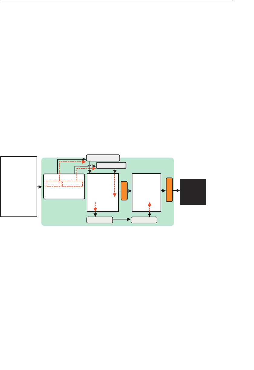
ptg11539634

Passing Other Types of Information to Vertex Shaders 149

At line 5 of the vertex shader, an attribute variable a_Color is declared in order to receive

the color data. Next, at line 6, a new varying variable

v_Color is declared that will be used

to pass its value to the fragment shader. Please note that you can only use float types (and

related types

vec2 , vec3 , vec4 , mat2 , mat3 , and mat4 ) for varying variables:

5 ‘attribute vec4 a_Color;n’ +

6 ‘varying vec4 v_Color;n’ +

At line 10, the value of a_Color is assigned to the variable v_Color declared at line 6:

10 ‘ v_Color = a_Color;n’ +

So how can the fragment shader receive the assigned data? The answer is straightforward.

All that is required is declaring a variable in the fragment shader with the same name and

types as that in the vertex shader:

18 ‘varying vec4 v_Color;n’ +

In WebGL, when varying variables declared inside the fragment shader have identical

names and types to the ones declared in the vertex shader, the assigned values in the

vertex shader are automatically passed to the fragment shader (see Figure 5.7 ).

gl_FragColor

{)(niamnoitcnuf

…LGbeWteg=lgrav

…

;)…(sredahStini

…

}

gl_Position

r =oloCgarF_lg

=noitisoP_lg

;noitisoP_a

;noitisoP_aetubirtta

;roloC_aetubirtta

reffuBroloC

metsySLGbeW

,0.0,0.0,0.1,5.0,0.0

,0.0,0.1,0.0,5.0—,5.0—

0.1,0.0,0.0,5.0—,5.0

redahSxetreV

oloC_v gniyrav

roloC_v gniyrav

v_Color;

v_Color = a_Color;

tnemgarF

redahS

tcejbOreffuB

tpircSavaJ

Figure 5.7 The behavior of a varying variable

So, the fragment shader can receive the values assigned to the vertex shader at

line 10 simply by assigning the varying variable

v_Color to gl_FragColor at line 20.

gl_FragColor sets the fragment color, the color of each point will be modified:

20 ‘ gl_FragColor = v_Color;n’ +

The remaining code is similar to MultiAttributeSize.js . The only differences are that

the name of the typed array for vertex information defined at line 58 is modified to

verticesColors , and the color information such as (1.0, 0.0, 0.0) is added to the data

definition at line 60.

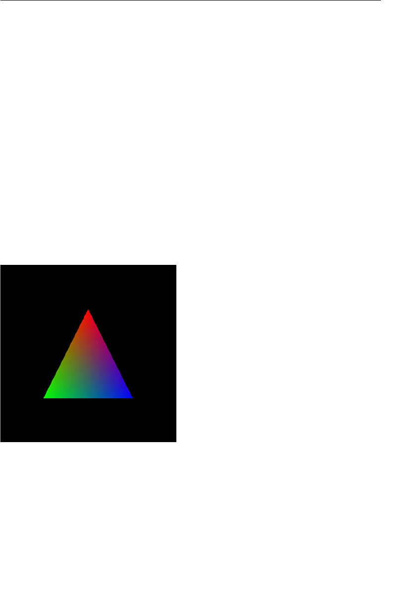
ptg11539634

CHAPTER 5 Using Colors and Texture Images

150

As previously explained in Chapter 2 , the color information is specified using the 0.0–1.0

range for each component of the RGBA model. Just like

MultiAttributeSize_Stride.

js , you store several different types of data within a single array. The fifth ( stride ) and

sixth ( offset ) arguments of

gl.vertexAttribPointer() are modified at lines 84 and 93,

respectively, based on the content of the

verticesColors array which, because you have

introduced some color information in addition to the vertex coordinates, means the stride

changes to

FSIZE * 5.

Finally, the draw command at line 54 results in red, blue, and green points being

displayed in the browser.

Experimenting with the Sample Program

Let’s modify the first argument of gl.drawArrays() at line 54 to gl.TRIANGLES and see

what happens upon execution. Alternatively, you can load the

ColoredTriangle sample

program from the book’s website:

54 gl.drawArrays(gl.TRIANGLES, 0, n);

The execution output is shown in Figure 5.8 . It might be difficult to grasp the difference

when seen in black and white, but on your screen, notice that a nice smooth-shaded

triangle with red, green, and blue corners is drawn.

Figure 5.8 ColoredTriangle

ptg11539634

Color Triangle (ColoredTriangle.js) 151

This significant change from three colored points to a smoothly shaded triangle occurred

just by changing one parameter value. Let’s look at how that came about.

Color Triangle (ColoredTriangle.js)

You already explored the subject of coloring triangles using a single color in Chapter 3 .

This section explains how to specify a different color for each of the triangle’s vertices and

the process within WebGL that results in a smooth color transition between the different

vertices.

To fully comprehend the phenomenon, you need to understand in detail the process

carried out between the vertex and the fragment shaders, as well as the functionality of

the varying variable.

Geometric Shape Assembly and Rasterization

Let’s start the explanation using the example program, HelloTriangle.js , introduced in

Chapter 3 , which simply draws a red triangle. The relevant code snippet necessary for the

explanation is shown in Listing 5.5 .

Listing 5.5 HelloTriangle.js (Code Snippet)

1 // HelloTriangle.js

2 // Vertex shader program

3 var VSHADER_SOURCE =

4 ‘attribute vec4 a_Position;n’ +

5 ‘void main() {n’ +

6 ‘ gl_Position = a_Position;n’ +

7 ‘}n’;

9 // Fragment shader program

10 var FSHADER_SOURCE =

11 ‘void main() {n’ +

12 ‘ gl_FragColor = vec4(1.0, 0.0, 0.0, 1.0);n’ +

13 ‘}n’;

15 function main() {

…

32 // Set vertex coordinates

33 var n = initVertexBuffers(gl);

…

45 // Draw a triangle

46 gl.drawArrays(gl.TRIANGLES, 0, n);

47 }

49 function initVertexBuffers(gl) {

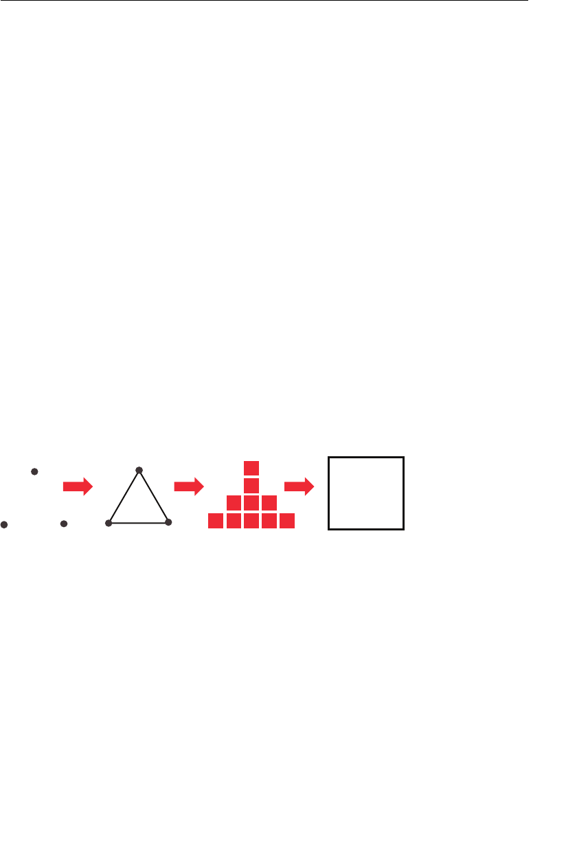
ptg11539634

CHAPTER 5 Using Colors and Texture Images

152

50 var vertices = new Float32Array([

51 0.0, 0.5, -0.5, -0.5, 0.5, -0.5

52 ]);

53 var n = 3; // The number of vertices

…

74 gl.vertexAttribPointer(a_Position, 2, gl.FLOAT, false, 0, 0);

…

81 return n;

82 }

In this program, after writing the vertex coordinates (lines 50 to 52) into the buffer object

in the function

initVertexBuffers() , the buffer object is assigned to the attribute variable

a_Position at line 74. Following that, when gl.drawArrays() invokes the vertex shader at

line 46, the three vertex coordinates inside the buffer object are passed to

a_Position at

line 4 and assigned to

gl_Position at line 6, thus making them available to the fragment

shader. In the fragment shader, the RGBA value (1.0, 0.0, 0.0, 1.0) associated with the red

color is assigned to

gl_FragColor , so a red triangle is displayed.

Up until now, you haven’t actually explored how this works, so let’s examine how exactly

a fragment shader performs per-fragment operations when you only give it the triangle’s

three vertex coordinates in

gl_Position .

In Figure 5.9 , you can see the problem. The program gives three vertices, but who identi-

fies that the vertex coordinates assigned to

gl_Position are the vertices of a triangle? In

addition, to make the triangle look like it is filled with a single color, who decides which

fragments have to be colored? Finally, who is responsible for invoking the fragment

shader and how it handles processing for each of the fragments?

= roloCgarF_lg

;roloC_v

tnemgarF

redahS

Figure 5.9 Vertex coordinate, identification of a triangle from the vertex coordinates,

rasterization, and execution of a fragment shader

Up until now, we have glossed over these details, but there are actually two processes

taking place between the vertex and the fragment shaders, which are shown in Figure

5.10 .

• The geometric shape assembly process: In this stage, the geometric shape is assem-

bled from the specified vertex coordinates. The first argument of

gl.drawArray()

specifies which type of shape should be assembled.

• The rasterization process: In this stage, the geometric shape assembled in the

geometric assembly process is converted into fragments.

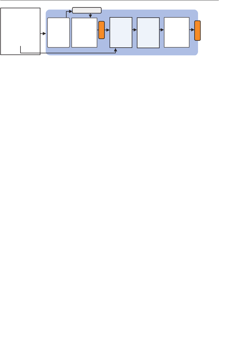
ptg11539634

Color Triangle (ColoredTriangle.js) 153

gl_FragColor

epahS

ylbmessA

aziretsaR

noit—

redahSxetreV

{)(niamnoitcnuf

…LGbeWteg=lgrav

syarrAward.lg

;)n,0,SELGNAIRT.lg(

noitisoP_aetubirtta

reffuB

tcejbO

5.0,0.0

5.0—,5.0—

5.0—,5.0

=noitisoP_lg

;noitisoP_a

=roloCgarF_lg

;)...(4cev

gl_Position

metsySLGbeW

tpircSavaJ

tnemgarF

redahS

Figure 5.10 Assembly and rasterization between a vertex shader and a fragment shader

As you will have realized from Figure 5.10 ,

gl_Position actually acts as the input to the

geometric shape assembly stage. Note that the geometric shape assembly process is also

called the primitive assembly process because the basic shapes previously shown in

Chapter 2 are also called primitives .

Figure 5.11 shows the processes between the vertex and fragment shaders, which are actu-

ally performed in assembly and rasterization for

HelloTriangle.js .

From Listing 5.5 , the third argument n of gl.drawArrays() (line 46) is set to 3, meaning

that the vertex shader is actually invoked three times.

Step 1. The vertex shader is invoked, and then the first coordinate (0.0, 0.5) inside the

buffer object is passed to the attribute variable

a_Position . Once this is assigned

gl_Position , this coordinate is communicated to the geometric shape assem-

bly stage and held there. As you will remember, because only the x and y coordi-

nates are passed to

a_Position , the z and w values are supplied, so actually (0.0,

0.5, 0.0,1.0) is held.

Step 2. The vertex shader is once again invoked, and in a similar way the second coordi-

nate (–0.5, –0.5) is passed to the geometric shape assembly stage and held there.

Step 3. The vertex shader is invoked a third time, passing the third coordinate (0.5, –0.5)

to the geometric shape assembly stage and holding it there.

Now the vertex shader processing is complete, and the three coordinates are

readily available for the geometric shape assembly stage.

Step 4. The geometric shape assembly processing starts. Using the three vertices

passed and the information (

gl.TRIANGLES ) contained in the first argument of

gl.drawArrays() , this stage decides how primitives should be assembled. In this

case, a triangle is assembled using the three vertices.

Step 5. Because what is displayed on the screen is a triangle consisting of fragments

(pixels), the geometric shape is converted to fragments. This process is called

rasterization . Here, the fragments that make up the triangle will be generated.

You can see the example of the generated fragments in the box of the rasteriza-

tion stage in Figure 5.11 .

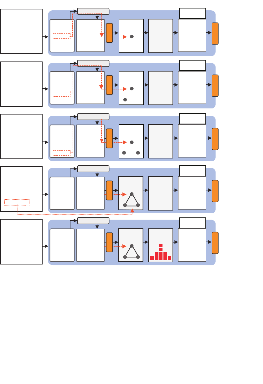
ptg11539634

CHAPTER 5 Using Colors and Texture Images

154

gl_FragColor

epahS ylbmessA

aziretsaR

noit—

redahSxetreV

tpircSavaJ

{)(niamnoitcnuf

…LGbeWteg=lgrav

syarrAward.lg

;)n,0,SELGNAIRT.lg(

noitisoP_aetubirtta

reffuB

tcejbO

5.0,0.0

5.0—,5.0—

5.0—,5.0

tnemgarF

redahS

=noitisoP_lg

;noitisoP_a

=roloCgarF_lg

;)...(4cev

)1(petS

gl_FragColor

epahS ylbmessA

aziretsaR

noit—

noitisoP_aetubirtta

reffuB

tcejbO

5.0,0.0

5.0—,5.0—

5.0—,5.0

tnemgarF

redahS

=noitisoP_lg

;noitisoP_a

=roloCgarF_lg

;)...(4cev

)2(petS

gl_Position gl_Position

gl_FragColor

epahS ylbmessA

aziretsaR

noit—

tpircSavaJ

{)(niamnoitcnuf

…LGbeWteg=lgrav

syarrAward.lg

;)n,0,SELGNAIRT.lg(

noitisoP_aetubirtta

5.0,0.0

5.0—,5.0—

5.0—,5.0

tnemgarF

redahS

=noitisoP_lg

;noitisoP_a

=roloCgarF_lg

;)...(4cev

)3(petS

gl_FragColor

epahS ylbmessA

aziretsaR

noit—

noitisoP_aetubirtta

5.0,0.0

5.0—,5.0—

5.0—,5.0

tnemgarF

redahS

=noitisoP_lg

;noitisoP_a

=roloCgarF_lg

;)...(4cev

)4(petS

{)(niamnoitcnuf

…LGbeWteg=lgrav

syarrAward.lg

;)n,0,SELGNAIRT.lg(

tpircSavaJ

gl_Position gl_Position

gl_FragColor

epahS ylbmessA

aziretsaR

noit—

noitisoP_aetubirtta

5.0,0.0

5.0—,5.0—

5.0—,5.0

tnemgarF

redahS

=noitisoP_lg

;noitisoP_a

=roloCgarF_lg

;)...(4cev

)5(petS

{)(niamnoitcnuf

…LGbeWteg=lgrav

syarrAward.lg

;)n,0,SELGNAIRT.lg(

tpircSavaJ

gl_Position

redahSxetreV

{)(niamnoitcnuf

…LGbeWteg=lgrav

syarrAward.lg

;)n,0,SELGNAIRT.lg(

tpircSavaJ

reffuB

tcejbO

reffuB

tcejbO

reffuB

tcejbO

Figure 5.11 The processing flow of geometric shape assembly and rasterization

In this figure, although we show only 10 fragments, the actual number of fragments is

determined according to the area where the triangle is finally displayed on the screen.

If you specify a different geometric shape in the first argument of

gl.drawArrays() , the

geometric shape assembled in Step 4 is modified accordingly, as are the number of frag-

ments and their position in Step 5. For example, if you specify

gl.LINES , a line will be

assembled out of the first two coordinates, and the remaining one will be discarded. If you

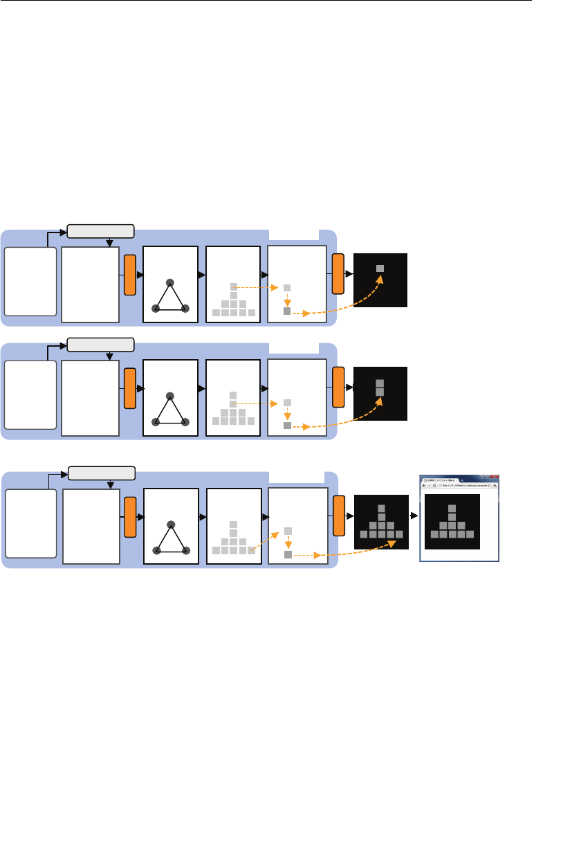
ptg11539634

Color Triangle (ColoredTriangle.js) 155

set it to gl.LINE_LOOP , a connected group of line segments will be generated, and only a

transparent (no fill color) triangle will be drawn.

Fragment Shader Invocations

Once the rasterization stage is completed, the fragment shader is invoked to process each

of the generated fragments. So in this example, the fragment shader is invoked 10 times,

as illustrated in Figure 5.12 . To avoid cluttering the figure, we skip the intermediate steps.

All of the fragments are fed one by one to the fragment shader, and for each fragment,

the fragment shader sets the color and writes its output to the color buffer. When the

last fragment shader process is completed at Step 15, the final output is displayed in the

browser.

Shape

Assembly

Rasteriza

-tion

Vertex

Shader

attribute a_Position

Buffer

Object

0.0, 0.5

-0.5, -0.5

0.5, -0.5

Fragment

Shader

gl_Position =

a_Position;

gl_FragColor =

vec4(…);

Step(6)

Shape

Assembly

Rasteriza

-tion

Vertex

Shader

attribute a_Position

Buffer

Object

0.0, 0.5

-0.5, -0.5

0.5, -0.5

Fragment

Shader

gl_Position =

a_Position;

gl_FragColor =

vec4(…);

Step(7)

Shape

Assembly

Rasteriza

-tion

Vertex

Shader

attribute a_Position

Buffer

Object

0.0, 0.5

-0.5, -0.5

0.5, -0.5

Fragment

Shader

gl_Position =

a_Position;

gl_FragColor =

vec4(…);

Step(15)

gl_Position

Color Buffer

…

gl_Position

gl_FragColor

Browser

Figure 5.12 Fragment shader invocations

The following fragment shader in

HelloTriangle.js colors each fragment in red. As a

result, a red filled triangle is written to the color buffer and displayed in the browser.

9 // Fragment shader program

10 var FSHADER_SOURCE =

11 ‘void main() {n’ +

12 ‘ gl_FragColor = vec4(1.0, 0.0, 0.0, 1.0);n’ +

13 ‘}n’;

ptg11539634

CHAPTER 5 Using Colors and Texture Images

156

Experimenting with the Sample Program

As an experiment, let’s confirm that the fragment shader is called for each fragment by

trying to set the color of each fragment based on its location. Each fragment generated by

the rasterization stage has its coordinates passed to the fragment shader upon invocation.

These coordinates can be accessed through the built-in variables provided inside the frag-

ment shader ( Table 5.1 ).

Table 5.1 Built-In Variables in a Fragment Shade (Input)

Type and Variable Name Description

vec4

gl_FragCoord The first and second component are the coordinates of the frag-

ment in the

<canvas> coordinate system (window coordinate

system)

To check that the fragment shader is actually executed for each fragment, you can modify

line 12 in the program, as follows:

1 // HelloTriangle_FragCoord.js

…

9 // Fragment shader program

10 var FSHADER_SOURCE =

11 ‘precision mediump float;n’ +

12 ‘uniform float u_Width;n’ +

13 ‘uniform float u_Height;n’ +

14 ‘void main() {n’ +

15 ‘ gl_FragColor = vec4(gl_FragCoord.x/u_Width, 0.0, gl_FragCoord.y/u_Height,

➥1.0);n’ +

16 ‘}n’;

As you can see, the color components of each fragment, red and blue, are calculated based

on the fragment’s coordinates on the canvas. Note that the canvas’s y-axis is the inverse

direction to the WebGL coordinate system, and because it’s in WebGL, the color value

is expressed in the 0.0 to 1.0 range, you can divide the coordinates by the size of the

<canvas> element (that is, 400 pixels) to get the appropriate color value. As you can see,

the width and height are passed into the shader using the uniform variables

u_Width and

u_Height and determined from gl.drawingBufferWidth and gl.drawingBufferHeight.

You can see the execution result in Figure 5.13 , which is a triangle whose fragments are

colored as a function of their position. Running this sample program

HelloTriangle_

FragCoord , you will see the transition from the left top to the right bottom.

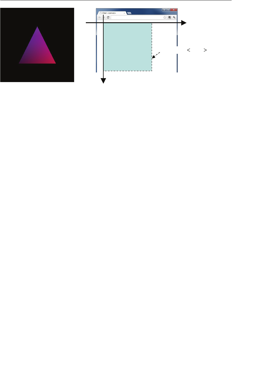
ptg11539634

Color Triangle (ColoredTriangle.js) 157

Drawing area of canvas

(0.0, 0.0)

(400, 400)

Figure 5.13 Modifying the color per fragment (the figure on the right side shows the <canvas>

coordinate system)

Because you modify the color of each fragment with respect to its coordinates, you will

notice that the color progressively changes according to the coordinates. Again, if this is

not clear from the black-and-white image in Figure 5.13 , run the example from the book’s

website.

Functionality of Varying Variables and the Interpolation Process

At this stage, you have a better understanding of the process flow taking place between

the vertex and the fragment shaders (that is, the geometric shape assembly process and

the subsequent rasterization process), as well as the invocation of the fragment shader for

each of the generated fragments.

Returning to Figure 5.8 , the first

ColoredTriangle , let’s use what you’ve learned to under-

stand better why you get such a nicely shaded triangle when you specify a different color

for each the triangle’s vertex. Previously, you saw that the value assigned to the varying

variable inside the vertex shader is passed as a varying variable with identical attributes

(same name, same type) to the fragment shader (see Figure 5.14 ). However, to be more

precise, the value assigned to the varying variable in the vertex shader is interpolated at

the rasterization stage. Consequently, the value passed to the fragment shader actually

differs for each fragment based on that interpolation (see Figure 5.15 ). This is the reason

the varying variable has the name “varying.”

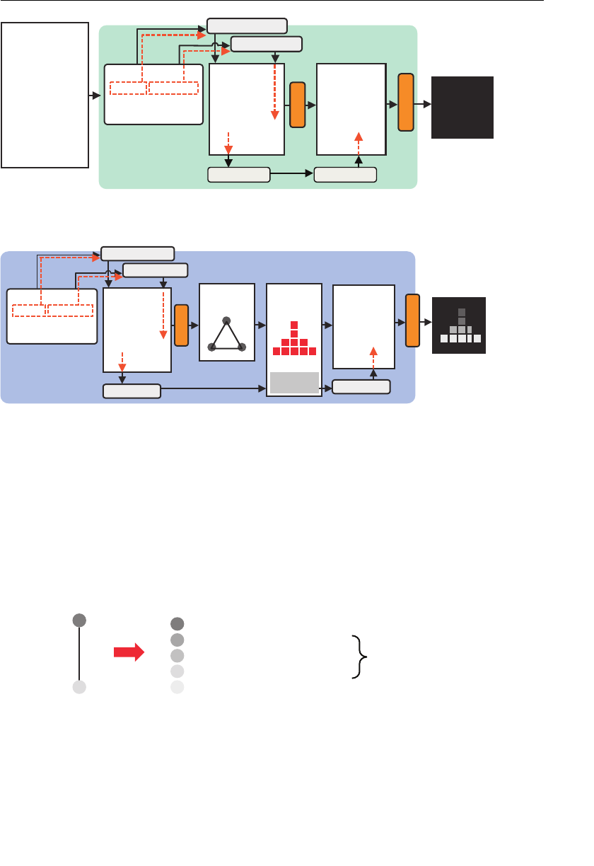
ptg11539634

CHAPTER 5 Using Colors and Texture Images

158

gl_FragColor

{)(niamnoitcnuf

…LGbeWteg=lgrav

…

;)…(sredahStini

…

}

gl_Position

r =oloCgarF_lg

=noitisoP_lg

;noitisoP_a

;noitisoP_aetubirtta

;roloC_aetubirtta

reffuBroloC

metsySLGbeW

,0.0,0.0,0.1,5.0,0.0

,0.0,0.1,0.0,5.0—,5.0—

0.1,0.0,0.0,5.0—,5.0

redahSxetreV

oloC_v gniyrav

roloC_v gniyrav

v_Color;

v_Color = a_Color;

tnemgarF

redahS

tcejbOreffuB

tpircSavaJ

Figure 5.14 The behavior of a varying variable (reprint of Figure 5.7 )

tnemgarF

redahS

gl_Position

;roloC_vgniyrav

redahSxetreV

=roloCgarF_lg

;roloC_v

=noitisoP_lg

;noitisoP_a

=roloC_v;roloC_a

;noitisoP_aetubirtta

;roloC_aetubirtta

,0.0,0.0,0.1,5.0,0.0

,0.0,0.1,0.0,5.0—,5.0—

0.1,0.0,0.0,5.0—,5.0

reffuBroloC

metsySLGbeW

gl_FragColor

epahS

ylbmessA

;roloC_vgniyrav

aziretsaR

noit

alopretnI

noit

tcejbOreffuB

Figure 5.15 Interpolation of a varying variable

More specifically, in

ColoredTriangle , because we only assign a different value to the

varying variable for each of the three vertices, each fragment located between vertices

must have its own color interpolated by the WebGL system.

For example, let’s consider the case in which the two end points of a line are specified

with different colors. One of the vertices is red (1.0, 0.0 0.0), whereas the other one is blue

(0.0, 0.0, 1.0). After the colors (red and blue) are assigned to the vertex shader’s

v_Color ,

the RGB values for each of the fragments located between those two vertices are calculated

and passed to the fragment shader’s

v_Color (see Figure 5.16 ).

deR

)0.0,0.0,0.1(

eulB

)0.1,0.0,0.0(

noitaziretsaR

aniroloC_v

redahsxetrev

detarenegsrolocehT

noitalopretniyb

)0.0,0.0,0.1(deR

)52.0,0.0,57.0(rolocdetalopretnI

)05.0,0.0,05.0(rolocdetalopretnI

)57.0,0.0,52.0(rolocdetalopretnI

)0.1,0.0,0.0(eulB

aniroloC_v

redahstnemgarf

Figure 5.16 Interpolation of color values

ptg11539634

Color Triangle (ColoredTriangle.js) 159

In this case, R decreases from 1.0 to 0.0, B increases from 0.0 to 1.0, and all the RGB

values between the two vertices are calculated appropriately—this is called the interpola-

tion process . Once the new color for each of the fragments located between the two verti-

ces is calculated in this way, it is passed to the fragment shader’s

v_Color .

We follow an identical procedure in the case of the colored triangle, which is reproduced

in Listing 5.6 . After the three vertices’ colors are assigned to the varying variable

v_Color

(line 9), the interpolated color for each fragment is passed to the fragment shader’s

v_Color . Once this is assigned to the gl_FragColor at line 19, a colored triangle is drawn,

as shown in Figure 5.8 . This interpolation process is carried out for each of the varying

variables. If you want to understand more about this process, a good source of informa-

tion is the book Computer Graphics .

Listing 5.6 ColoredTriangle.js

1 // ColoredTriangle.js

2 // Vertex shader program

3 var VSHADER_SOURCE = ‘

…

6 varying vec4 v_Color;

7 void main() {

8 gl_Position = a_Position;

9 v_Color = a_Color; <- The color at line 59 is assigned to v_Color

10 }’;

12 // Fragment shader program

13 var FSHADER_SOURCE =

…

17 varying vec4 v_Color; <- The interpolated color is passed to v_Color

18 void main() {

19 gl_FragColor = v_Color; <- The color is assigned to gl_FragColor

20 }’;

22 function main() {

…

53 gl.drawArrays(gl.TRIANGLES, 0, n);

54 }

56 function initVertexBuffers(gl) {

57 var verticesColors = new Float32Array([

58 // Vertex coordinates and color

59 0.0, 0.5, 1.0, 0.0, 0.0,

60 -0.5, -0.5, 0.0, 1.0, 0.0,

61 0.5, -0.5, 0.0, 0.0, 1.0,

62 ]);

…

99 }

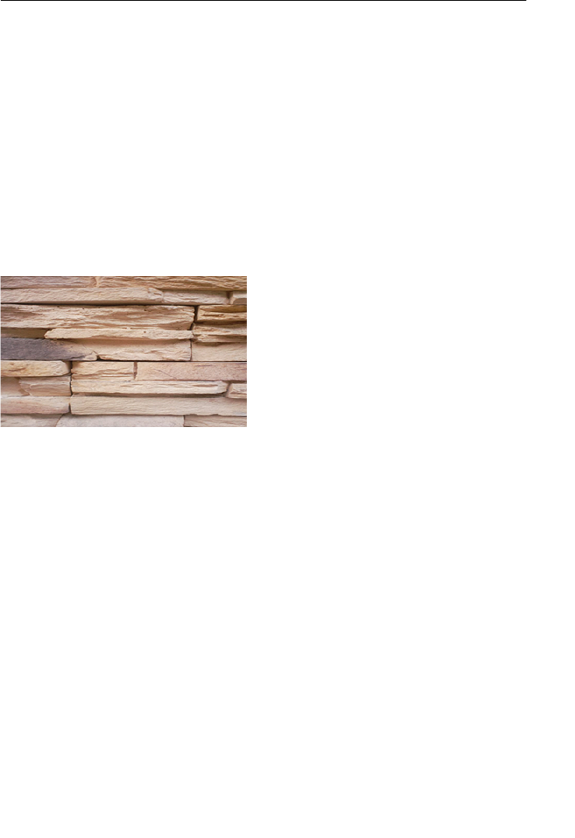
ptg11539634

CHAPTER 5 Using Colors and Texture Images

160

In summary, this section has highlighted the critical rasterization process that takes place

between the vertex and fragment shaders. Rasterization is a key component of 3D graph-

ics and is responsible for taking geometric shapes and building up the fragments that will

draw those shapes. After converting the specified geometric shape into fragments (raster-

ization), it’s possible to set a different color for each of the fragments inside the fragment

shader. This color can be interpolated or set directly by the programmer.

Pasting an Image onto a Rectangle

In the previous section, you explored how to use color when drawing shapes and how

interpolation creates smooth color transitions. Although powerful, this approach is limited

when it comes to reproducing complex visual representations. For example, a problem

arises if you want to create a wall that has the look and feel of the one shown in Figure

5.17 , you would need many triangles, and determining the color and coordinates for each

triangle would prove to be daunting.

Figure 5.17 An example of a complex wall surface

As you’d imagine, in 3D graphics, one of the most important processes is actually solving

this problem. The problem is resolved using a technique called texture mapping , which

can re-create the look of real-world materials. The process is actually straightforward and

consists of pasting an image (like a decal) on the surface of a geometrical shape. By pasting

an image from a real-world photograph on a rectangle made up of two triangles, you can

give the rectangle surface an appearance similar to that of a picture. The image is called a

texture image or a texture .

The role of the texture mapping process is to assign the texture image’s pixel colors to the

fragments generated by the rasterization process introduced in the previous section. The

pixels that make up the texture image are called texels (texture elements), and each texel

codes its color information in the RGB or RGBA format (see Figure 5.18 ).

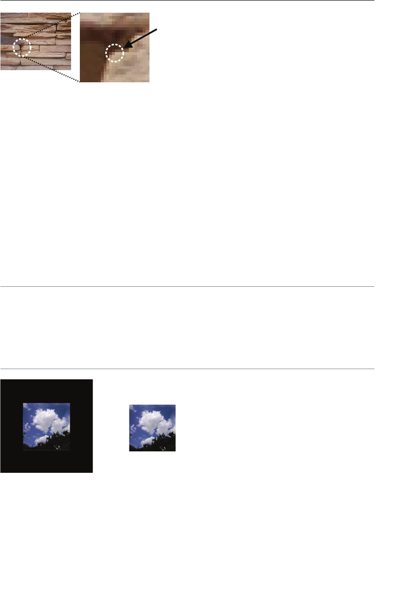
ptg11539634

Pasting an Image onto a Rectangle 161

Enlargement

Each square is a texel

Figure 5.18 Texels

Texture mapping involves the following four steps in WebGL:

1. Prepare the image to be mapped on the geometric shape.

2. Specify the image mapping method for the geometric shape.

3. Load the texture image and configure it for use in WebGL.

4. Extract the texels from the image in the fragment shader, and accordingly set the

corresponding fragment.

To understand the mechanisms involved in texture mapping, let’s examine the sample

program

TextureQuad , which “pastes” an image onto a rectangle. If you run it from the

book’s website, you’ll see the result as shown in Figure 5.19 (left).

Note When you want to run the sample programs that use texture images in Chrome

from your local disk, you should add the option

—allow-file-access-from-files to

Chrome. This is for security reasons. Chrome, by default, does not allow access to local

files such as

../resources/sky.jpg . For Firefox, the equivalent parameter, set via

about:config , is security.fileuri.strict_origin_policy , which should be set to

false . Remember to set it back when you’re finished because you open a security loop-

hole if local file access is enabled.

sky.jpg

Texture image

Figure 5.19 TextureQuad (left) and the texture image used (right)

Looking in a little more detail at steps (1) to (4) in the following sections, the image

prepared in (1) can be any format that can be displayed in a browser. For now, you can

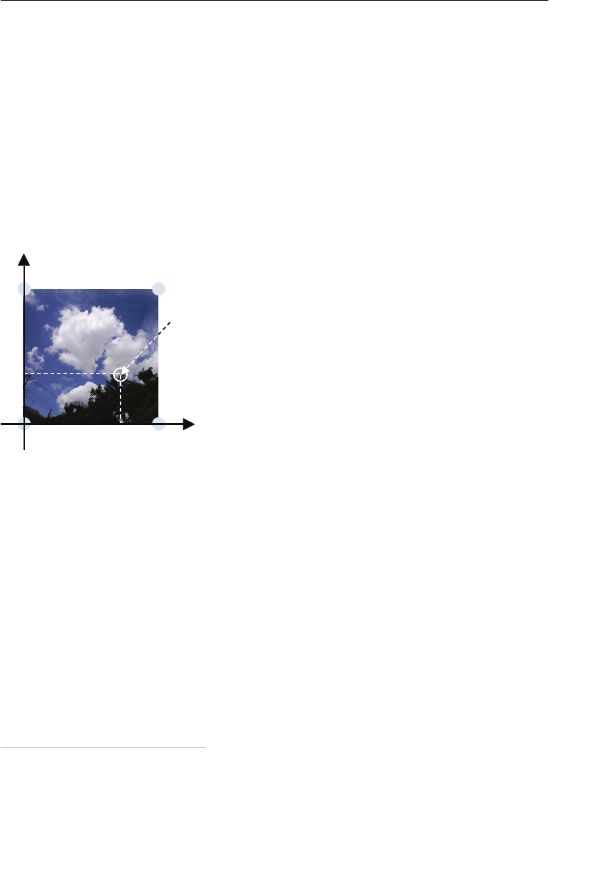
ptg11539634

CHAPTER 5 Using Colors and Texture Images

162

use any pictures you might have taken yourself or alternatively you can use the images

located in the

resource folder of the companion website provided with this book.

The mapping method specified in (2) consists of designating “which part of the texture

image” should be pasted to “which part of the geometric shape”. The part of the geomet-

ric shape meant to be covered with the texture is specified using the coordinates of the

vertices that compose a surface. The part of the texture image to be used is specified using

texture coordinates . These are a new form of coordinates so let’s look at how they work.

Texture Coordinates

The texture coordinate system used in WebGL is two-dimensional, as shown in Figure

5.20 . To differentiate the texture coordinates from the widely used x and y axis, WebGL

changes the denomination to the s and t coordinates (st coordinates system).

Texture Image

Text at the texture coordinate

(0.7, 0.4)

(0.0, 1.0)

(0.0, 0.0) (1.0, 0.0)

(1.0, 1.0)

Figure 5.20 WebGL’s Texture coordinate system

As you can see from Figure 5.20 , the coordinates of the four corners are defined as left

bottom corner (0.0, 0.0), right bottom corner (1.0, 0.0), right top corner (1.0, 1.0), and

left top corner (0.0, 1.0). Because these values are not related to the image size, this allows

a common approach to image handling; for example, whether the texture image’s size is

128×128 or 128×256, the right top corner coordinates will always be

(1.0, 1.0).

Pasting Texture Images onto the Geometric Shape

As previously mentioned, in WebGL, by defining the correspondence between the texture

coordinates and the vertex coordinates of the geometric shape, you can specify how the

texture image will be pasted (see Figure 5.21 ).

2 The uv coordinates are often used. However, we are using st coordinates because GLSL ES uses the

component names to access the texture image.

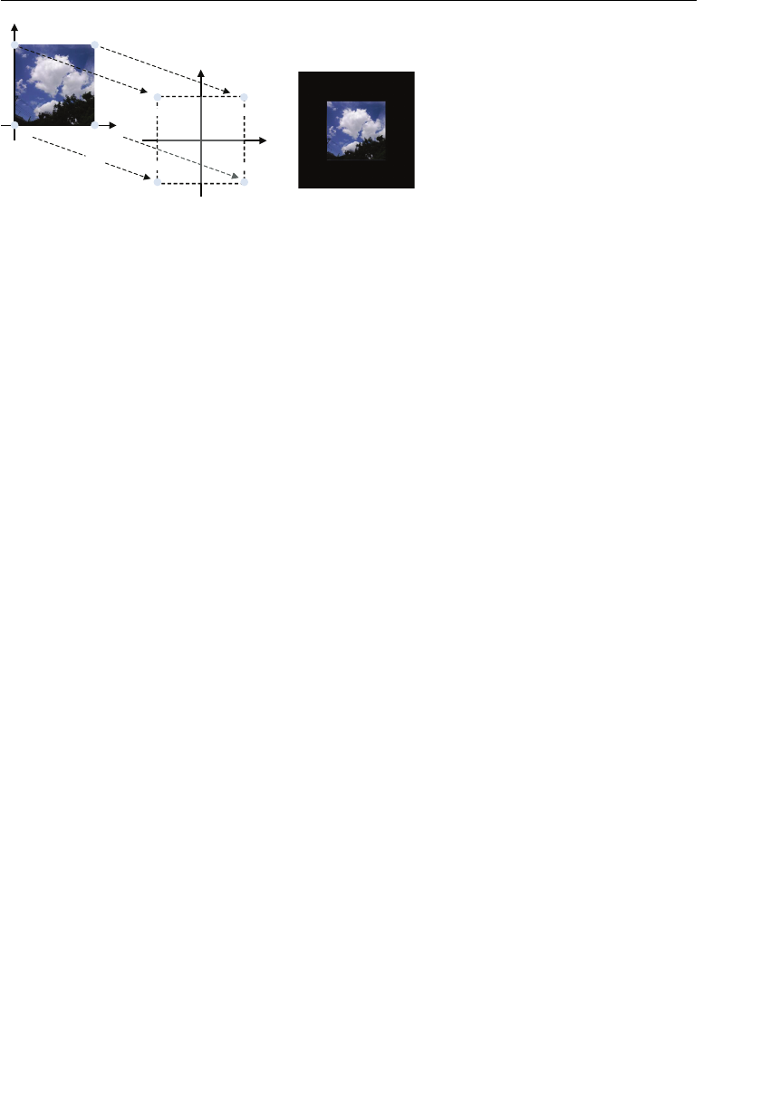
ptg11539634

Pasting an Image onto a Rectangle 163

Texture coordinate system

WebGL coordinate system The resulting image produced by WebGL

(0.0, 1.0)

(0.0, 0.0) (1.0, 0.0)

(1.0, 1.0)

(-05, 0.5, 0.0) (05, 0.5, 0.0)

(-05, -0.5, 0.0) (05, -0.5, 0.0)

Figure 5.21 Texture coordinates and mapping them to vertices

Here, the texture coordinates (0.0, 1.0) are mapped onto the vertex coordinates (–0.5, 0.5,

0.0), and the texture coordinates (1.0, 1.0) are mapped onto the vertex coordinates (0.5,

0.5, 0.0). By establishing the correspondence for each of the four corners of the texture

image, you obtain the result shown in the right part of Figure 5.21 .

Now, given your understanding of how images can be mapped to shapes, let’s look at the

sample program.

Sample Program (TexturedQuad.js)

In TexturedQuad.js (see Listing 5.7 ), the texture mapping affects both the vertex and the

fragment shaders. This is because it sets the texture coordinates for each vertex and then

applies the corresponding pixel color extracted from the texture image to each fragment.

There are five main parts to the example, each identified by the numbers to the right of

the code.

Listing 5.7 TexturedQuad.js

1 // TexturedQuad.js

2 // Vertex shader program <- (Part1)

3 var VSHADER_SOURCE =

4 ‘attribute vec4 a_Position;n’ +

5 ‘attribute vec2 a_TexCoord;n’ +

6 ‘varying vec2 v_TexCoord;n’ +

7 ‘void main() {n’ +

8 ‘ gl_Position = a_Position;n’ +

9 ‘ v_TexCoord = a_TexCoord;n’ +

10 ‘}n’;

12 // Fragment shader program <- (Part2)

13 var FSHADER_SOURCE =

…

17 ‘uniform sampler2D u_Sampler;n’ +

18 ‘varying vec2 v_TexCoord;n’ +

19 ‘void main() {n’ +

ptg11539634

CHAPTER 5 Using Colors and Texture Images

164

20 ‘ gl_FragColor = texture2D(u_Sampler, v_TexCoord);n’ +

21 ‘}n’;

23 function main() {

…

40 // Set the vertices information <- (Part3)

41 var n = initVertexBuffers(gl);

…

50 // Setting the textures

51 if (!initTextures(gl, n)) {

…

54 }

55 }

57 function initVertexBuffers(gl) {

58 var verticesTexCoords = new Float32Array([

59 // Vertices coordinates, textures coordinates

60 -0.5, 0.5, 0.0, 1.0,

61 -0.5, -0.5, 0.0, 0.0,

62 0.5, 0.5, 1.0, 1.0,

63 0.5, -0.5, 1.0, 0.0,

64 ]);

65 var n = 4; // The number of vertices

67 // Create the buffer object

68 var vertexTexCoordBuffer = gl.createBuffer();

…

74 // Write the vertex coords and textures coords to the object buffer

75 gl.bindBuffer(gl.ARRAY_BUFFER, vertexTexCoordBuffer);

76 gl.bufferData(gl.ARRAY_BUFFER, verticesTexCoords, gl.STATIC_DRAW);

78 var FSIZE = verticesTexCoords.BYTES_PER_ELEMENT;

…

85 gl.vertexAttribPointer(a_Position, 2, gl.FLOAT, false, FSIZE * 4, 0);

86 gl.enableVertexAttribArray(a_Position); // Enable buffer allocation

88 // Allocate the texture coordinates to a_TexCoord, and enable it.

89 var a_TexCoord = gl.getAttribLocation(gl.program, ‘a_TexCoord’);

…

94 gl.vertexAttribPointer(a_TexCoord, 2, gl.FLOAT, false, FSIZE * 4, FSIZE * 2);

95 gl.enableVertexAttribArray(a_TexCoord); // Enable buffer allocation

…

97 return n;

98 }

ptg11539634

Pasting an Image onto a Rectangle 165

100 function initTextures(gl, n) <- (Part4)

101 var texture = gl.createTexture(); // Create a texture object

…

107 // Get the storage location of the u_Sampler

108 var u_Sampler = gl.getUniformLocation(gl.program, ‘u_Sampler’);

…

114 var image = new Image(); // Create an image object

…

119 // Register the event handler to be called on loading an image

120 image.onload = function(){ loadTexture(gl, n, texture, u_Sampler, image); };

121 // Tell the browser to load an image

122 image.src = ‘../resources/sky.jpg’;

123

124 return true;

125 }

126

127 function loadTexture(gl, n, texture, u_Sampler, image){ <- (Part5)

128 gl.pixelStorei(gl.UNPACK_FLIP_Y_WEBGL, 1); // Flip the image’s y axis

129 // Enable the texture unit 0

130 gl.activeTexture(gl.TEXTURE0);

131 // Bind the texture object to the target

132 gl.bindTexture(gl.TEXTURE_2D, texture);

133

134 // Set the texture parameters

135 gl.texParameteri(gl.TEXTURE_2D, gl.TEXTURE_MIN_FILTER, gl.LINEAR);

136 // Set the texture image

137 gl.texImage2D(gl.TEXTURE_2D, 0, gl.RGB, gl.RGB, gl.UNSIGNED_BYTE, image);

138

139 // Set the texture unit 0 to the sampler

140 gl.uniform1i(u_Sampler, 0);

…

144 gl.drawArrays(gl.TRIANGLE_STRIP, 0, n); // Draw a rectangle

145 }

This program is structured into five main parts:

Part 1: Receive the texture coordinates in the vertex shader and then pass them to the

fragment shader.

Part 2: Paste the texture image onto the geometric shape inside the fragment shader.

Part 3: Set the texture coordinates (

initVertexBuffers() ).

Part 4: Prepare the texture image for loading, and request the browser to read it.

(

initTextures() ).

Part 5: Configure the loaded texture so that it can be used in WebGL ( loadTexture() ).

ptg11539634

CHAPTER 5 Using Colors and Texture Images

166

Let’s look at the sequence starting from Part 3: the process to set the texture coordinates

using

initVertexBuffers() . The shaders are executed after loading the image, so we will

explain them at the end.

Using Texture Coordinates (initVertexBuffers())

You pass texture coordinates to the vertex shader using the same approach you’ve been

using to pass other vertex data to the vertex shader, by combining vertex coordinates and

vertex data into a single buffer. Line 58 defines an array

verticesTexCoords containing

pairs of vertex coordinates and their associated texture coordinates:

58 var verticesTexCoords = new Float32Array([

59 // Vertex coordinates and texture coordinates

60 -0.5, 0.5, 0.0, 1.0,

61 -0.5, -0.5, 0.0, 0.0,

62 0.5, 0.5, 1.0, 1.0,

63 0.5, -0.5, 1.0, 0.0,

64 ]);

As you can see, the first vertex (–0.5, 0.5) is mapped to the texture coordinate (0.0, 1.0),

the second vertex (–0.5, –0.5) is mapped to the texture coordinate (0.0, 0.0), the third

vertex (0.5, 0.5) is mapped to the texture coordinate (1.0, 10), and the fourth vertex (0.5,

–0.5) is mapped to the texture coordinate (1.0, 0.0). Figure 5.21 illustrates these mappings.

Lines 75 to 86 then write vertex coordinates and texture coordinates to the buffer object,

assign it to

a_Position , and enable the assignment. After that, lines 89 to 94 retrieve the

storage location of the attribute variable

a_TexCoord and then assign the buffer object

containing the texture coordinates to the variable. Finally, line 95 enables the assignment

of the buffer object to

a_TexCoord :

88 // Assign the texture coordinates to a_TexCoord, and enable it.

89 var a_TexCoord = gl.getAttribLocation(gl.program, ‘a_TexCoord’);

…

94 gl.vertexAttribPointer(a_TexCoord, 2, gl.FLOAT, false, FSIZE * 4,

➥FSIZE * 2);

95 gl.enableVertexAttribArray(a_TexCoord);

Setting Up and Loading Images (initTextures())

This process is performed from lines 101 to 122 in initTextures() . Line 101 creates

a texture object (

gl.createTexture() ) for managing the texture image in the WebGL

system, and line 108 gets the storage location of a uniform variable (

gl.getUniformLoca-

tion() ) to pass the texture image to the fragment shader () :

101 var texture = gl.createTexture(); // Create a texture object

…

108 var u_Sampler = gl.getUniformLocation(gl.program, ‘u_Sampler’);

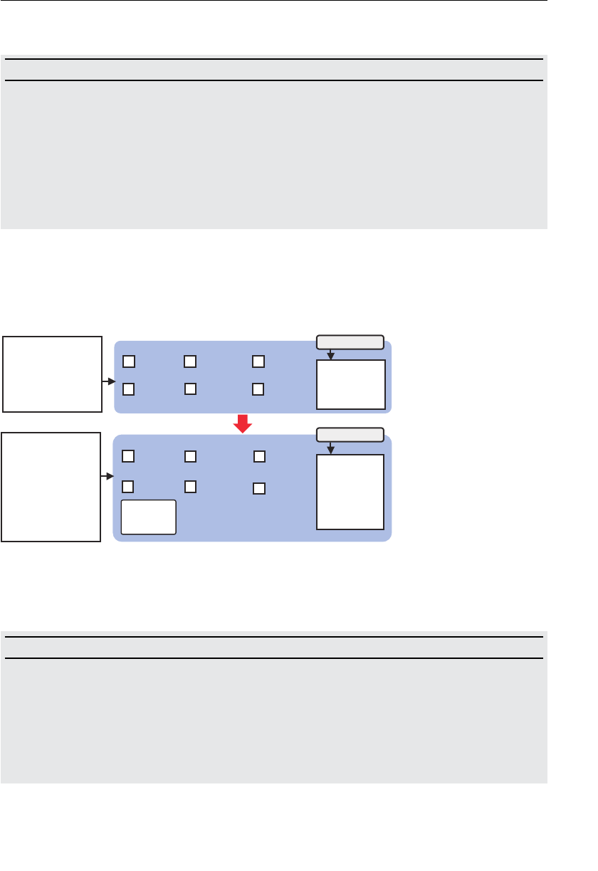
ptg11539634

Pasting an Image onto a Rectangle 167

A texture object is created using gl.createTexture() .

gl.createTexture()

Create a texture object to hold a texture image.

Parameters None

Return value non-null The newly created texture object.

null Failed to create a texture object.

Errors None

This call creates the texture object in the WebGL system, as shown in Figure 5.22 .

gl.TEXTURE0 to gl.TEXTURE7 are texture units for managing a texture image, and each has

an associated

gl.TEXTURE_2D , which is the texture target for specifying the type of texture.

This will be explained in detail later.

tnemgarF

redahS

elbairavmrofinu

tpircSavaJ

{)(niamnoitcnuf

…LGbeWteg=lgrav

…

0ERUTXET.lg …1ERUTXE

T.lg 7ERUTXET.lg

…

tnemgarF

redahS

erutxeT

tcejbO

tpircSavaJ

{)(niamnoitcnuf

…LGbeWteg=lgrav

…

;)…(erutxeTetaerc.lg

…1ERUTXET.lg0ERUTXET.lg 7ERUTXET.l

_ERUTXET.l

…

D2_ERUTXET.lg

D2_ERUTXET.lg D2_ERUTXET.lg

D2_ER

TXET

D2_ERUTXET.lg

Figure 5.22 Create a texture object

The texture object can be deleted using

gl.deleteTexture() . Note, if this method is called

with a texture object that has already been deleted, the call has no effect.

gl.deleteTexture(texture)

Delete the texture object specified by texture.

Parameter texture Specifies the texture object to be deleted.

Return value None

Errors None

ptg11539634

CHAPTER 5 Using Colors and Texture Images

168

In the next step, it’s necessary to request that the browser load the image that will be

mapped to the rectangle. You need to use an

Image object for this purpose:

114 var image = new Image() ; // Create an Image object

…

119 // Register an event handler to be called when image loading completes

120 image.onload = function(){ loadTexture(gl, n, texture, u_Sampler, image); };

121 // Tell the browser to load an image

122 image.src = ‘../resources/sky.jpg’;

This code snippet creates an Image object, registers the event handler ( loadTexture() ) to

be called on loading the image, and tells the browser to load the image.

You need to create an

Image object (a special JavaScript object that handles images) using

the

new operator, just as you would do for an Array object or Date object. This is done at

line 114.

114 var image = new Image(); // Create an Image object

Because loading of images is performed asynchronously (see the boxed article that

follows), when the browser signals completion of loading, it needs to pass the image

to the WebGL system. Line 120 handles this, telling the browser that, after loading the

image, the anonymous function

loadTexture() should be called.

120 image.onload = function(){ loadTexture(gl, n, texture, u_Sampler, image ); };

loadTexture() takes five parameters, with the newly loaded image being passed via

the variable (

Image object) as the last argument image . gl is the rendering context for

WebGL,

n is the number of vertices, texture is the texture object created at line 101, and

u_Sampler is the storage location of a uniform variable.

Just like the <img> tag in HTML, we can tell the browser to load the texture image by

setting the image filename to the property

src of the Image object (line 122). Note that

WebGL, because of the usual browser security restrictions, is not allowed to use images

located in other domains for texture images:

122 image.src = ‘../resources/sky.jpg’;

After executing line 122, the browser starts to load the image asynchronously, so the

program continues on to the

return statement at line 124 and then exits. When the

browser finishes loading the image and wants to pass the image to the WebGL system, the

event handler

loadTexture() is called.

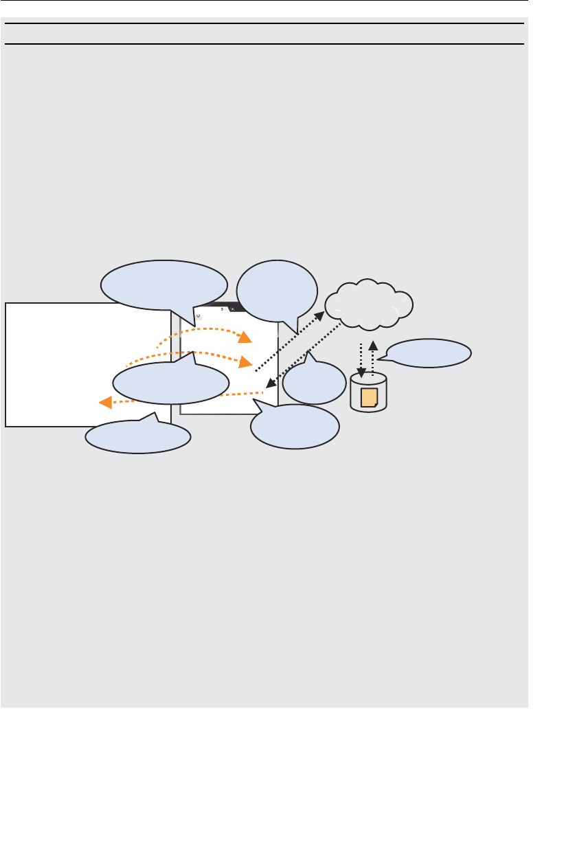
ptg11539634

Pasting an Image onto a Rectangle 169

Asynchronous Loading Texture Images

Usually, OpenGL applications written in C or C++ load the texture image files straight

from the hard disk where they are stored. However, because WebGL programs are

running inside the browser, it is impossible to load images directly. Instead, it is

necessary to read images indirectly by requesting the browser to do it. (Typically, the

browser sends a request to the web server to obtain the image.) The advantage is that

you can use any kind of image a browser can display, but it also makes the process

more complex because you now have to handle two processes (the browser loading

request, and the actual WebGL loading) that behave “asynchronously” (they run in the

background) and thus do not block execution of the program.

Figure 5.23 shows the substeps between [1] tell the browser to load an image and [7] call

the function

loadTexture() after completing loading the texture image.

JavaScript

{)(serutxeTtini

…

.egaminagnidaolnotneveehtretsigeR//

;};)…(erutxeTdaol{)(noitcnuf=daolno.egami

.egaminad

aolotresworbehtlleT//

;‘gpj.yks/secruoser/..‘=crs.egami

…

}

{)…(erutxeTdaolnoitcnuf

…

}

llacotresworbehtlleT]1[

gnidaolretfa)(erutxeTdaol

.egamina

.)(erutxeTdaolllaC]7[

otresworbehtlleT]2[

.egaminadaol

beW

revres

.egamidaoL]4[

Image file

)gpj.yks(

[

etelpmoC

nagniveirter

.egami

ehttseuqeR]3[

otrevresbeW

naeveirter

.egami

etelpmoC]6[

.egaminagnidaol

resworB

Figure 5.23 Asynchronous loading texture images

In Figure 5.23 , [1] and [2] are executed sequentially, but [2] and [7] are not. After

requesting the browser to load an image in [2], the JavaScript program doesn’t wait for

the image to be loaded, but proceeds to the next stage. (This behavior will be explained

in detail in a moment.) While the JavaScript program is continuing, the browser

sends a request to the web server for the image [3]. When the image loading process is

completed [4] and [5], the browser tells the JavaScript program that the image loading

has completed [6]. This kind of behavior is referred to as asynchronous .

The image loading process is analogous to the way a web page written in HTML displays

images. In HTML, an image is displayed by specifying the file URL to the

src attribute of

the

<img> tag (below) causing the browser to load the image from the specified URL. This

part corresponds to [2] shown in Figure 5.23 .

ptg11539634

CHAPTER 5 Using Colors and Texture Images

170

The asynchronous nature of the image loading process can be easily understood by

considering how a web page that includes numerous images is displayed. Typically,

the page text and layout are displayed rapidly, and then images appear slowly as

they are loaded. This is because the image loading and display processes are executed

asynchronously, allowing you to view and interact with the web page without having to

wait for all images to load.

Make the Texture Ready to Use in the WebGL System (loadTexture())

The function loadTexture() is defined as follows:

127 function loadTexture(gl, n, texture, u_Sampler, image) { <- (Part5)

128 gl.pixelStorei(gl.UNPACK_FLIP_Y_WEBGL, 1); // Flip the image’s y axis

129 // Enable the texture unit 0

130 gl.activeTexture(gl.TEXTURE0);

131 // Bind the texture object to the target

132 gl.bindTexture(gl.TEXTURE_2D, texture);

133

134 // Set the texture parameters

135 gl.texParameteri(gl.TEXTURE_2D, gl.TEXTURE_MIN_FILTER, gl.LINEAR);

136 // Set the texture image

137 gl.texImage2D(gl.TEXTURE_2D, 0, gl.RGB, gl.RGB, gl.UNSIGNED_BYTE, image);

138

139 // Set the texture unit 0 to the sampler

140 gl.uniform1i(u_Sampler, 0);

…

144 gl.drawArrays(gl.TRIANGLE_STRIP, 0, n); // Draw a rectangle

145 }

Its main purpose is to prepare the image for use by the WebGL system, which it does

using a texture object that is prepared and used in a similar manner to a buffer object.

The following sections explain the code in more detail.

Flip an Image’s Y—Axis

Before using the loaded images as a texture, you need to flip the y-axis:

128 gl.pixelStorei(gl.UNPACK_FLIP_Y_WEBGL, 1);// Flip the image’s y-axis

This method flips an image’s Y-axis when it’s loaded. As shown in Figure 5.24 , the t-axis

direction of the WebGL texture coordinate system is the inverse of the y-axis direction of

the coordinate system used by PNG, BMP, JPG, and so on. For this reason, if you flip the

image’s Y-axis, you can map the image to the shape correctly. (You could also flip the t

coordinates by hand instead of flipping the image.)

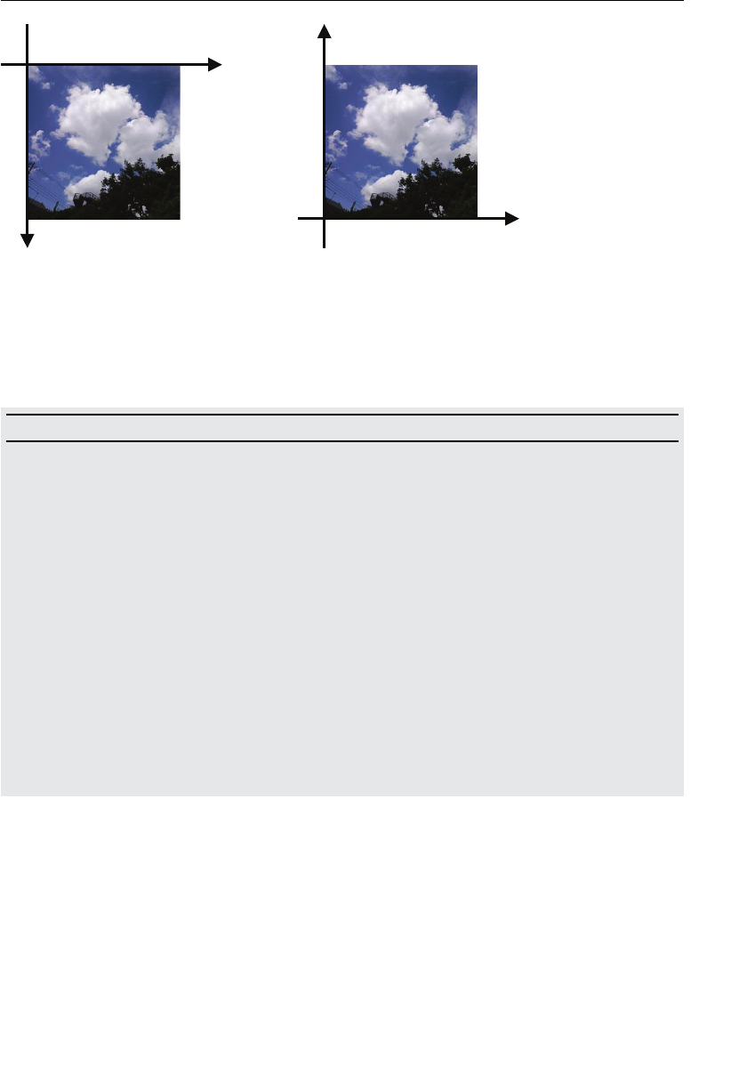
ptg11539634

Pasting an Image onto a Rectangle 171

WebGL coordinate system

Image coordinate system

Figure 5.24 The image coordinate system and WebGL texture coordinate system

The following explains

gl.pixelStorei() .

gl.pixelStorei(pname, param)

Perform the process defined by pname and param after loading an image.

Parameters pname Specifies any of the following:

gl.UNPACK_FLIP_Y_WEBGL Flips an image’s Y-axis after loading the

image. The default value is

false .

gl.UNPACK_PREMULTIPLY_

ALPHA_WEBGL

Multiplies each component of RGB in an

image by A in the image. The default value is

false .

param Specifies none-zero (means

true ) or zero

(means

false ). It must be specified in the

integer.

Return value None

Errors INVALID_ENUM pname is none of these values.

Making a Texture Unit Active (gl.activeTexture())

WebGL supports multiple texture images (multitexturing) using a mechanism called

a texture unit . A texture unit manages texture images by using a unit number for each

texture. Because of this, even if you only want to use a single texture image, you must

specify and use a texture unit.

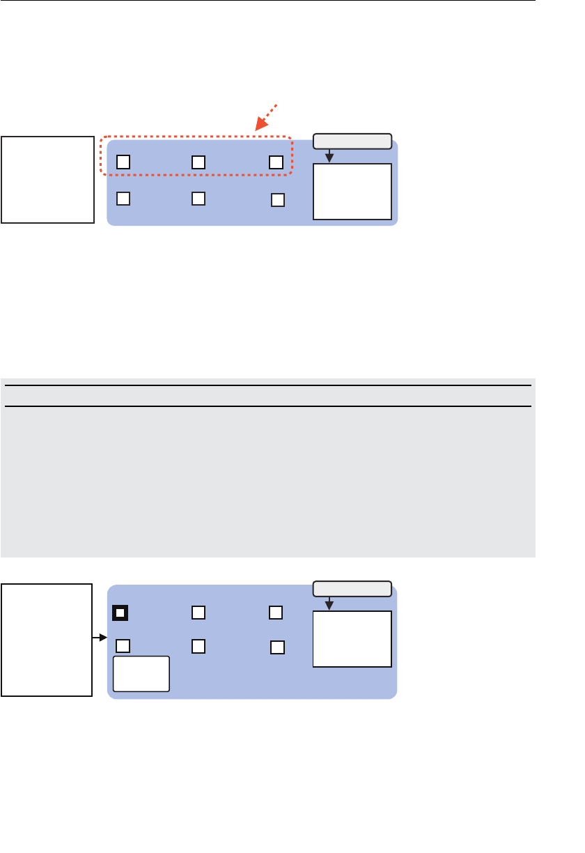
ptg11539634

CHAPTER 5 Using Colors and Texture Images

172

The number of texture units supported varies according to your hardware and WebGL

implementation, but by default at least eight texture units are supported, and some

systems will support more. The built-in constants,

gl.TEXTURE0 , gl.TEXTURE1 , …, and

gl.TEXTURE7 , represent each texture unit (see Figure 5.25 ).

tnemgarF

redahS

elbairavmrofinu

tpircSavaJ

{)(niamnoitcnuf

…LGbeWteg=lgrav

…

D2_ERUTXET.lg

Texture unit

…1ERUTXET.lg0ERUTXET.lg 7ERUTXET.lg

D2_ERUTXET.lg D2_ERUTXET.lg

Figure 5.25 Multiple texture units managed by WebGL

Before using a texture unit, it must be made active using a call to

gl.activeTexture() (see

Figure 5.26 ):

132 // Make the texture unit 0 active

133 gl.activeTexture(gl.TEXTURE0);

gl.activeTexture(texUnit)

Make the texture unit specified by texUnit active.

Parameters texUnit Specifies the texture unit to be made active:

gl.TEXTURE0 ,

gl.TEXTURE1 , …, or gl.TEXTURE7 . The tailing number indi-

cates the texture unit number.

Return value None

Errors INVALID_ENUM: texUnit is none of these values

tnemgarF

redahS

elbairavmrofinu

D2_ERUTXET.lg

…1ERUTXET.lg0ERUTXET.lg 7ERUTXET.lg

D2_ERUTXET.lg D2_ERUTXET.lg

erutxeT

tcejbO

;)…(erutxeTevitca.lg

tpircSavaJ

…LGbeWteg=lgrav

…

{)(niamnoitcnuf

Figure 5.26 Activate texture unit (gl.TEXTURE0)

ptg11539634

Pasting an Image onto a Rectangle 173

Binding a Texture Object to a Target (gl.bindTexture())

Next, you need to tell the WebGL system what types of texture image is used in the

texture object. You do this by binding the texture object to the target in a similar way to

that of the buffer objects explained in the previous chapter. WebGL supports two types of

textures, as shown in Table 5.2 .

Table 5.2 Types of Textures

Type of Texture Description

gl.TEXTURE_2D Two-dimensional texture

gl.TEXTURE_CUBE_MAP Cube map texture

The sample program uses a two-dimensional image as a texture and specifies

gl.

TEXTURE_2D at line 132. The cube map texture is beyond the scope of this book. If you are

interested in more information, please refer to the book OpenGL ES 2.0 Programming Guide :

131 // Bind the texture object to the target

132 gl.bindTexture(gl.TEXTURE_2D, texture);

gl.bindTexture(target, texture)

Enable the texture object specified by texture and bind it to the target . In addition, if a

texture unit was made active by

gl.activeTexture() , the texture object is also bound to

the texture unit.

Parameters target Specifies gl.TEXTURE_2D or gl.TEXTURE_CUBE_MAP .

texture Specifies the texture object to be bound.

Return value None

Errors INVALID_ENUM target is none of these values.

Note that this method performs two tasks: enabling the texture object and binding it

to target, and binding it to the texture unit. In this case, because the texture unit 0

(

gl.TEXTURE0 ) is active, after executing line 136, the internal state of the WebGL

system is changed, as shown in Figure 5.27 .

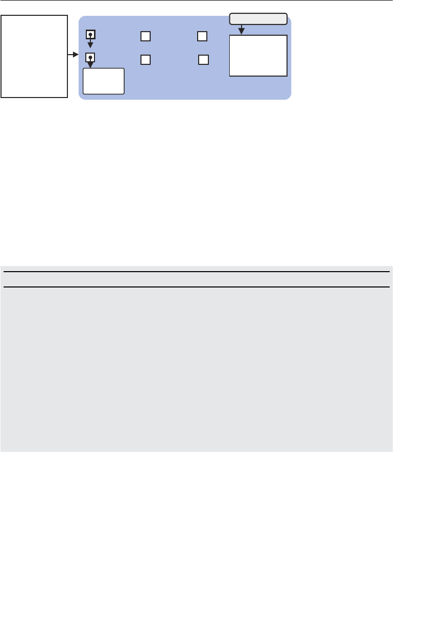
ptg11539634

CHAPTER 5 Using Colors and Texture Images

174

tnemgarF

redahS

elbairavmrofinu

…1ERUTXET.lg0ERUTXET.lg 7ERUTXET.lg

D2_ERUTXET.l

gD2_ERUTXET.l

erutxeT

tcejbO

tpircSavaJ

…LGbeWteg=lgrav

…

{)(niamnoitcnuf

;)…(erutxeTdnib.lg

D2_ERUTXET.lg

Figure 5.27 Bind a texture object to the target

At this stage, the program has specified the type of texture that is used in the texture

object (

gl.TEXTURE_2D ) and that will be used to deal with the texture object in the future.

This is important, because in WebGL, you cannot manipulate the texture object directly.

You need to do that through the binding.

Set the Texture Parameters of a Texture Object (gl.texParameteri())

In the next step, you need to set the parameters (texture parameter) that specify how the

texture image will be processed when the texture image is mapped to shapes. The generic

function

gl.texParameteri() can be used to set texture parameters.

gl.texParameteri(target, pname, param)

Set the value specified by param to the texture parameter specified by pname in the

texture object bound to target .

Parameters target Specifies

gl.TEXTURE_2D or gl.TEXTURE_CUBE_MAP .

pname Specifies the name of the texture parameter ( Table 5.3 ).

param Specifies the value set to the texture parameter pname

( Table 5.4 , Table 5.5 ).

Return value None

Errors INVALID_ENUM target is none of the preceding values

INVALID_OPERATION no texture object is bound to target

There are four texture parameters available, illustrated in Figure 5.28 , which you can

specify to pname :

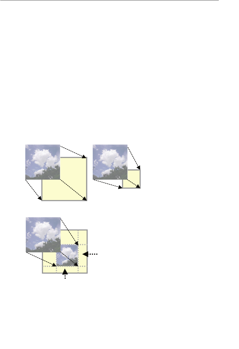
ptg11539634

Pasting an Image onto a Rectangle 175

• Magnification method ( gl.TEXTURE_MAG_FILTER ): The method to magnify a texture

image when you map the texture to a shape whose drawing area is larger than the

size of the texture. For example, when you map a 16×16 pixel image to a 32×32 pixel

shape, the texture should be doubled in size. WebGL needs to fill the gap between

texels due to the magnification, and this parameter specifies the method used to fill

the gap.

• Minification method ( gl.TEXTURE_MIN_FILTER ): The method of minifying a texture

image when you map the texture to a shape whose drawing area is smaller than

the size of the texture. For example, when you map a 32×32 pixel image to a 16×16

pixel shape, the texture should be reduced in size. To do that, the system needs to

cull texels to fit the target size. This parameter specifies the method used to cull

texels.

• Wrapping method on the left and right side ( gl.TEXTURE_WRAP_S ): How to fill the

remaining regions on the left side and the right side of a subregion when you map a

texture image to the subregion of a shape.

• Wrapping method on top and bottom ( gl.TEXTURE_WRAP_T ): Similar to (3), the

method used to fill the remaining regions in the top and bottom of a subregion.

The method to fill this region.

gl.TEXTURE_MAG_FILTER

gl.TEXTURE_WRAP_T

gl.TEXTURE_MIN_FILTER

gl.TEXTURE_WRAP_S

Magnification

Minification

The method to fill this region.

Figure 5.28 Four texture parameters and their effects

Table 5.3 shows each texture parameter and its default value.

ptg11539634

CHAPTER 5 Using Colors and Texture Images

176

Table 5.3 Texture Parameters and Their Default Values

Texture Parameter Description Default Value

gl.TEXTURE_MAG_FILTER Texture magnification gl.LINEAR

gl.TEXTURE_MIN_FILTER Texture minification gl.NEAREST_MIPMAP_LINEAR

gl.TEXTURE_WRAP_S Texture wrapping in s-axis gl.REPEAT

gl.TEXTURE_WRAP_T Texture wrapping in t-axis gl.REPEAT

We also show the constant values that can be specified to

gl.TEXTURE_MAG_FILTER and

gl.TEXTURE_MIN_FILTER in Table 5.4 and gl.TEXTURE_WRAP_S and gl.TEXTURE_WRAP_T in

Table 5.5 .

Table 5.4 Non-Mipmapped Values, Which Can be Specified to gl.TEXTURE_MAG_FILTER and

gl.TEXTURE_MIN_FILTER

Value Description

gl.NEAREST Uses the value of the texel that is nearest (in Manhattan distance) the center

of the pixel being textured.

gl.LINEAR Uses the weighted average of the four texels that are nearest the center

of the pixel being textured. (The quality of the result is clearer than that of

gl.NEAREST , but it takes more time.)

Table 5.5 Values that Can be Specified to gl.TEXTURE_WRAP_S and gl.TEXTURE_WRAP_T

Value Description

gl.REPEAT Use a texture image repeatedly

gl.MIRRORED_REPEAT Use a texture image mirrored-repeatedly

gl.CLAMP_TO_EDGE Use the edge color of a texture image

As shown in Table 5.3 , each parameter has a default value, and you can generally use the

default value as is. However, the default value of

gl.TEXTURE_MIN_FILTER is for a special

texture format called MIPMAP . A MIPMAP is a sequence of textures, each of which is

a progressively lower resolution representation of the same image. Because a MIPMAP

texture is not often used, we don’t cover it in this book. For this reason, you set the value

gl.LINEAR to the texture parameter gl.TEXTURE_MIN_FILTER at line 135:

3 Although omitted in this table, other values can be speci ed for a MIPMAP texture: gl.NEAREST_

MIPMAP_NEAREST , gl.LINEAR_MIPMAP_NEAREST , gl.NEAREST_MIPMAP_LINEAR , and gl.LINEAR_

MIPMAP_LINEAR . See the book OpenGL Programming Guide for these values.

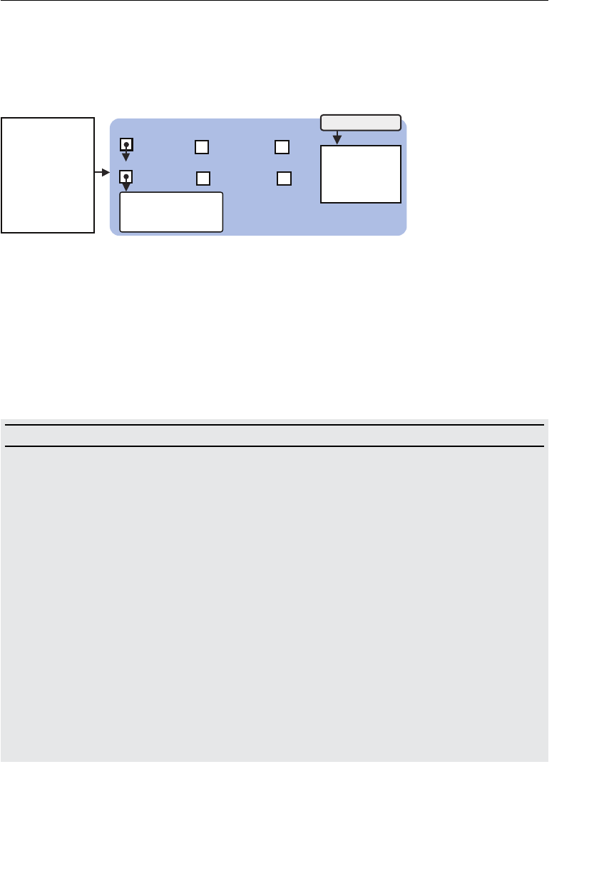
ptg11539634

Pasting an Image onto a Rectangle 177

134 // Set the texture parameters

135 gl.texParameteri(gl.TEXTURE_2D, gl.TEXTURE_MIN_FILTER, gl.LINEAR);

After executing line 139, the value is set to the texture object, and then the internal state

of the WebGL system is modified as shown in Figure 5.29 .

tnemgarF

redahS

elbairavmrofinu

…1ERUTXET.lg0ERUTXET.lg

ERUTXET.lg

D2_ERUTXET.lg D2_ERUTXET.lg

tpircSavaJ

…LGbeWteg=lgrav

…

{)(niamnoitcnuf

.D2_ERUTXET

tcejbOerutxeT

R E T L I F _ N I M _ E R U T X E T . l g

R A E N I L . l g

;)…(iretemaraPxet.lg

Figure 5.29 Set texture parameter

The next step is to assign a texture image to the texture object.

Assigning a Texture Image to a Texture Object (gl.texImage2D())

To assign an image to a texture object, you use the method gl.texImage2D() . In addition

to assigning a texture, this method allows you to tell the WebGL system about the image

characteristics.

gl.texImage2D(target, level, internalformat, format, type, image)

Set the image specified by image to the texture object bound to target.

Parameters target Specifies

gl.TEXTURE_2D or gl.TEXTURE_CUBE_MAP .

level Specified as 0. (Actually, this parameter is used for a

MIPMAP texture, which is not covered in this book.)

internalformat Specifies the internal format of the image ( Table 5.6 ).

format Specifies the format of the texel data. This must be

specified using the same value as internalformat .

type Specifies the data type of the texel data ( Table 5.7 ).

image Specifies an Image object containing an image to be

used as a texture.

Return value None

Errors INVALID_ENUM target is none of the above values.

INVALID_OPERATION No texture object is bound to target

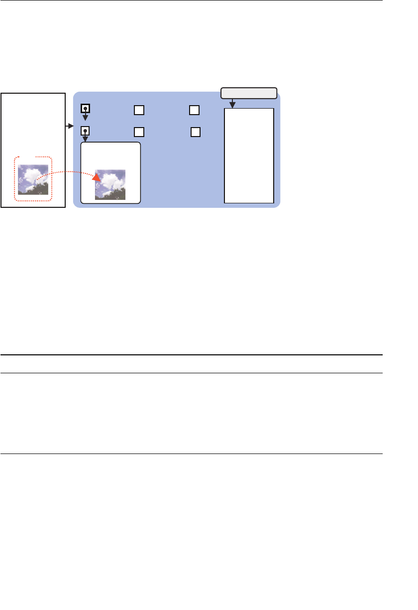
ptg11539634

CHAPTER 5 Using Colors and Texture Images

178

This method is used at line 136 in the sample program:

137 gl.texImage2D(gl.TEXTURE_2D, 0, gl.RGBA, gl.RGBA, gl.UNSIGNED_BYTE, image);

After executing line 144, the texture image loaded into the Image object image in

JavaScript is passed to the WebGL system (see Figure 5.30 ).

elbairavmrofinu

…1ERUTXET.lg0ERUTXET.lg 7ERUTXET.lg

D2_ERUTXET.lg D2_ERUTXET.lg

.D2_ERUTXETlg

egami

tpircSavaJ

…LGbeWteg=lgrav

…

{)(niamnoitcnuf

;)…(D2egamIxet.lg

tcejbOerutxeT

RETLIF_NIM_ERUTXET.l

RAENIL.lg

tnemgarF

redahS

Figure 5.30 Assign an image to the texture object

Let’s take a quick look at each parameter of this method. You must specify 0 to level

because you aren’t using a MIPMAP texture. The format specifies the format of the texel

data, with available formats shown in Table 5.6 . You need to select an appropriate format

for the image used as a texture. The sample program uses

gl.RGB format because it uses a

JPG image in which each pixel is composed of RGB components. For other formats, such

as PNG, images are usually specified as

gl.RGBA , and BMP images are usually specified as

gl.RGB . gl.LUMINANCE and gl.LUMINANCE_ALPHA are used for a grayscale image and so on.

Table 5.6 The Format of the Texel Data

Format Components in a Texel

gl.RGB Red, green, blue

gl.RGBA Red, green, blue, alpha

gl.ALPHA (0.0, 0.0, 0.0, alpha)

gl.LUMINANCE L, L, L, 1 L: Luminance

gl.LUMINANCE_ALPHA L, L. L. alpha

Here, luminance is the perceived brightness of a surface. It is often calculated as a

weighted average of red, green, and blue color values that gives the perceived brightness

of the surface.

As shown in Figure 5.30 , this method stores the image in the texture object in the WebGL

system. Once stored, you must tell the system about the type of format the image uses

ptg11539634

Pasting an Image onto a Rectangle 179

using the internalformat parameter. As mentioned, in WebGL, internalformat must specify

the same value as format .

The type specifies the data type of the texel data (see Table 5.7 ). Usually, we specify

gl.

UNSIGNED_BYTE as the data type. Other data types are also available, such as gl.UNSIGNED_

SHORT_5_6_5 (which packs RGB components into 16 bits). These types are used for passing

compressed images to the WebGL system to reduce loading time.

Table 5.7 The Data Type of Texel Data

Type Description

gl.UNSIGNED_BYTE Unsigned byte format. Each color component has 1 byte.

gl.UNSIGNED_SHORT_5_6_5 RGB: Each component has 5, 6, and 5 bits, respectively.

gl.UNSIGNED_SHORT_4_4_4_4 RGBA: Each component has 4, 4, 4, and 4 bits, respectively.

gl.UNSIGNED_SHORT_5_5_5_1 RGBA: Each RGB component has 5 bits, and A has 1 bit.

Pass the Texture Unit to the Fragment Shader (gl.uniform1i())

Once the texture image has been passed to the WebGL system, it must be passed to the

fragment shader to map it to the surface of the shape. As explained before, a uniform vari-

able is used for this purpose because the texture image does not change for each fragment:

13 var FSHADER_SOURCE =

…

17 ‘uniform sampler2D u_Sampler;n’ +

18 ‘varying vec2 v_TexCoord;n’ +

19 ‘void main() {n’ +

20 ‘ gl_FragColor = texture2D(u_Sampler, v_TexCoord);n’ +

21 ‘}n’;

This uniform variable must be declared using the special data type for textures shown in

Table 5.8 . The sample program uses a two-dimensional texture (

gl.TEXTURE_2D ), so the

data type is set to

sampler2D .

Table 5.8 Special Data Types for Accessing a Texture

Type Description

sampler2D Data type for accessing the texture bound to

gl.TEXTURE_2D

samplerCube Data type for accessing the texture bound to

gl.TEXTURE_CUBE_MAP

The call to

initTextures() (line 100) gets the storage location of this uniform variable

u_Sampler at line 108 and then passes it to loadTexture() as an argument. The uniform

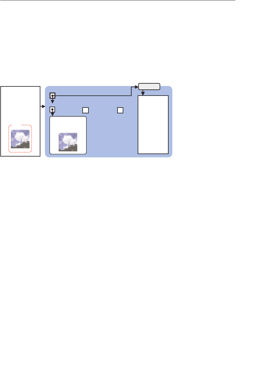
ptg11539634

CHAPTER 5 Using Colors and Texture Images

180

variable u_Sampler is set at line 139 by specifying the texture unit number (“n” in

gl.TEXTURE n ) of the texture unit that manages this texture object. In this sample program,

you specify 0 because you are using the texture object bound to

gl.TEXTURE0 in the call to

gl.uniformi() :

138 // Set the texture unit 0 to the sampler

139 gl.uniform1i(u_Sampler, 0);

After executing line 139, the WebGL system is modified as shown in Figure 5.31 , thereby

allowing access to the image in the texture object from the fragment shader.

tpircSavaJ

…LGbeWteg=lgrav

…

{)(niamnoitcnuf

;)…(D2egamIxet.lg

tcejbOerutxeT

RETLIF_NIM_ERUTXET.l

RAENIL.lg

tnemgarF

redahS

relpmaS_u

…1ERUTXET.lg0ERUTXET.lg 7ERUTXET.lg

D2_ERUTXET.lgD2_ERUTXET.lg

.D2_ERUTXETlg

egami

Figure 5.31 Set texture unit to uniform variable

Passing Texture Coordinates from the Vertex Shader to the Fragment

Shader

Because the texture coordinates for each vertex are passed to the attribute variable

a_TexCoord , it’s possible to pass the data to the fragment shader through the varying

variable

v_TexCoord . Remember that varying variables of the same name and type are

automatically copied between the vertex shader and the fragment shader. The texture

coordinates are interpolated between vertices, so you can use the interpolated texture

coordinates in a fragment shader to specify each texture coordinate for each fragment:

2 // Vertex shader program

3 var VSHADER_SOURCE =

4 ‘attribute vec4 a_Position;n’ +

5 ‘attribute vec2 a_TexCoord;n’ +

6 ‘varying vec2 v_TexCoord;n’ +

7 ‘void main() {n’ +

8 ‘ gl_Position = a_Position;n’ +

9 ‘ v_TexCoord = a_TexCoord;n’ +

10 ‘}n’;

At this stage, you have completed the preparations for using the texture image in the

WebGL system.

ptg11539634

Pasting an Image onto a Rectangle 181

All that’s left is to read the color of the texel located at the corresponding texture coordi-

nates from the texture image and then use it to set the color of the fragment.

Retrieve the Texel Color in a Fragment Shader (texture2D())

Retrieving a color of a texel from the texture image is done at line 20 in the fragment

shader:

20 ‘ gl_FragColor = texture2D(u_Sampler, v_TexCoord);n’ +

It uses the GLSL ES built-in function texture2D() to read out the texel color from the

shader.

texture2D() is an easy-to-use function that can retrieve the texel color at a texture

coordinate by specifying the texture unit number in the first parameter and the texture

coordinates in the second parameter. However, because this function is a built-in function

of GLSL ES, note the data type of the parameters and the return value of the function.

vec4 texture2D(sampler2D sampler, vec2 coord)

Retrieve a texel color at the texture coordinates specified by coord from the texture image

specified by sampler.

Parameters sampler Specifies the texture unit number.

coord Specifies the texture coordinates.

Return value The texel color (

vec4 ) for the coordinates. The color format changes accord-

ing to the internalformat specified by

gl.texImage2D() . Table 5.9 shows

the differences. If the texture image is not available for some reason, this

function returns (0.0, 0.0, 0.0, 1.0).

Table 5.9 Return Value of texture2D()

Internalformat Return Value

gl.RGB (R, G, B, 1.0)

gl.RGBA (R, G, B, A)

gl.ALPHA (0.0, 0.0, 0.0, A)

gl.LUMINANCE (L, L, L, 1.0) L indicates luminance

gl.LUMINANCE_ALPHA (L, L, L, A)

The texture magnification and minification parameters determine the return value in cases

where WebGL interpolates the texel. Once this function executes, by assigning the return

value to

gl_FragColor , the fragment is displayed using the color. As a result of this opera-

tion, the texture image is mapped to the shape to be drawn (in this case, a rectangle).

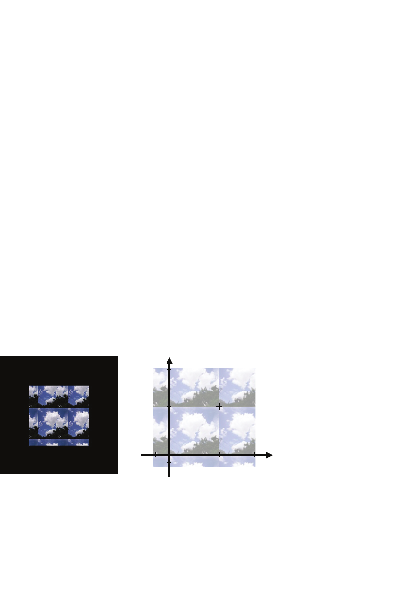
ptg11539634

CHAPTER 5 Using Colors and Texture Images

182

This is the final step in the process needed for texture mapping. At this stage, your texture

image has been loaded, set up in the WebGL system and mapped to the shape you are

drawing.

As you have seen, texture mapping in WebGL seems a complex process partly because it

must deal with an image and request the browser to load it, and partly because you are

required to use the texture unit even if you use only a single texture. However, once you

master the basic steps, they are the same each time you want to map a texture.

The next section explores the use of textures and will familiarize you with the whole

process.

Experimenting with the Sample Program

To familiarize you with texture mapping, let’s modify the sample program by changing

the texture coordinates. For example, modify the texture coordinates in

TexturedQuad as

follows:

var verticesTexCoords = new Float32Array([

// Vertex coordinates and texture coordinates

-0.5, 0.5, -0.3, 1.7,

-0.5, -0.5, -0.3, -0.2,

0.5, 0.5, 1.7, 1.7,

0.5, -0.5, 1.7, -0.2

]);

If you load the modified program TexturedQuad_Repeat , you’ll see an effect like the

screenshot of Figure 5.32 (left side). To understand what’s happening here, take a look at

the figure on the right side, which shows each texture coordinate in the texture coordi-

nate system.

(0.0,0.0) (1.0,0.0)

(0.0,1.0) (1.0,1.0)

-0.2-0.3

1.7

1.7 s

Figure 5.32 Modify the texture coordinate (a screenshot of TexturedQuad_Repeat)

The image isn’t sufficient to cover the larger shape, so as you can see, the texture image is

being repeated. This is driven by the value of

gl.TEXTURE_WRAP_S and gl.TEXTURE_WRAP_T ,

ptg11539634

Pasting Multiple Textures to a Shape 183

which are set to gl.REPEAT in the sample program, telling the WebGL system to repeat the

texture image to fill the area.

Now let’s modify the texture parameters as follows to see what other effects we can

achieve. The modified program is saved as

TexturedQuad_Clamp_Mirror , and Figure 5.33

shows the result when run in your browser:

// Set texture parameters

gl.texParameteri(gl.TEXTURE_2D, gl.TEXTURE_MIN_FILTER, gl.LINEAR );

gl.texParameteri(gl.TEXTURE_2D, gl.TEXTURE_WRAP_S, gl.CLAMP_TO_EDGE );

gl.texParameteri(gl.TEXTURE_2D, gl.TEXTURE_WRAP_T, gl.MIRRORED_REPEAT );

You can see that the edge color of the texture is repeated in the s-axis (horizontal axis),

and the texture image itself is mirrored-repeated in the t-axis (vertical axis).

Figure 5.33 TexturedQuad_Clamp_Mirror

That concludes the explanation of the basic texture mapping technique available in

WebGL. The next section builds on this basic technique and explores texture mapping

using multiple texture images.

Pasting Multiple Textures to a Shape

Earlier in the chapter, you learned that WebGL can deal with multiple texture images,

which was the reason for the multiple texture units. The examples so far have used

only one texture, and thus one element of the unit. This section will construct a sample

program,

MultiTexture , which pastes two texture images to a rectangle, allowing a

better examination of the texture unit mechanism. Figure 5.34 shows a screenshot of

MultiTexture . As you can see, the two texture images are “blended” to create the compos-

ite in the figure.

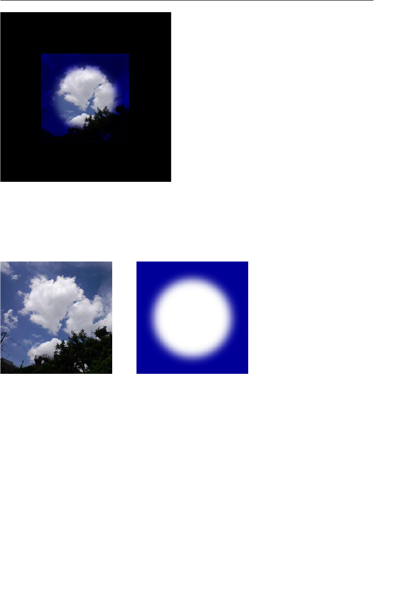
ptg11539634

CHAPTER 5 Using Colors and Texture Images

184

Figure 5.34 MultiTexture

Figure 5.35 shows the two separate texture images used in this sample program. To high-

light WebGL’s ability to deal with various image formats, the sample program intention-

ally uses different image formats for each file.

Figure 5.35 Texture images (sky.jpg on left; circle.gif on right) used in MultiTexture

Essentially, you can map multiple texture images to a shape by repeating the process of

mapping a single texture image to a shape described in the previous section. Let’s examine

the sample program to see how that is done.

Sample Program (MultiTexture.js)

Listing 5.8 shows the basic processing flow of MultiTexture.js , which is similar to

TexturedQuad.js with three key differences: (1) the fragment shader accesses two textures,

(2) the final fragment color is calculated from the two texels from both textures, and (3)

initTextures() creates two texture objects.

ptg11539634

Pasting Multiple Textures to a Shape 185

Listing 5.8 MultiTexture.js

1 // TexturedQuad.js

…

13 var FSHADER_SOURCE =

…

17 ‘uniform sampler2D u_Sampler0;n’ +

18 ‘uniform sampler2D u_Sampler1;n’ +

19 ‘varying vec2 v_TexCoord;n’ +

20 ‘void main() {n’ +

21 ‘ vec4 color0 = texture2D(u_Sampler0, v_TexCoord);n’ + <-(1)

22 ‘ vec4 color1 = texture2D(u_Sampler1, v_TexCoord);n’ +

23 ‘ gl_FragColor = color0 * color1;n’ + <-(2)

24 ‘}n’;

26 function main() {

…

53 // Set textures

54 if (!initTextures(gl, n)) {

…

58 }

60 function initVertexBuffers(gl) {

61 var verticesTexCoords = new Float32Array([

62 // Vertex coordinates and texture coordinates

63 -0.5, -0.5, 0.0, 1.0,

64 -0.5, -0.5, 0.0, 0.0,

65 0.5, -0.5, 1.0, 1.0,

66 0.5, -0.5, 1.0, 0.0,

67 ]);

68 var n = 4; // The number of vertices

…

100 return n;

101 }

102

103 function initTextures(gl, n) {

104 // Create a texture object

105 var texture0 = gl.createTexture(); <-(3)

106 var texture1 = gl.createTexture();

…

112 // Get the storage locations of u_Sampler1 and u_Sampler2

113 var u_Sampler0 = gl.getUniformLocation(gl.program, ‘u_Sampler0’);

114 var u_Sampler1 = gl.getUniformLocation(gl.program, ‘u_Sampler1’);

…

120 // Create Image objects

ptg11539634

CHAPTER 5 Using Colors and Texture Images

186

121 var image0 = new Image();

122 var image1 = new Image();

…

127 // Register the event handler to be called when image loading is completed

128 image0.onload = function(){ loadTexture(gl, n, texture0, u_Sampler0,

➥image0, 0); };

129 image1.onload = function(){ loadTexture(gl, n, texture1, u_Sampler1,

➥image1, 1); };

130 // Tell the browser to load an Image

131 image0.src = ‘../resources/redflower.jpg’;

132 image1.src = ‘../resources/circle.gif’;

133

134 return true;

135 }

136 // Specify whether the texture unit is ready to use

137 var g_texUnit0 = false, g_texUnit1 = false ;

138 function loadTexture(gl, n, texture, u_Sampler, image, texUnit) {

139 gl.pixelStorei(gl.UNPACK_FLIP_Y_WEBGL, 1);// Flip the image’s y-axis

140 // Make the texture unit active

141 if (texUnit == 0) {

142 gl.activeTexture(gl.TEXTURE0);

143 g_texUnit0 = true;

144 } else {

145 gl.activeTexture(gl.TEXTURE1);

146 g_texUnit1 = true;

147 }

148 // Bind the texture object to the target

149 gl.bindTexture(gl.TEXTURE_2D, texture);

150

151 // Set texture parameters

152 gl.texParameteri(gl.TEXTURE_2D, gl.TEXTURE_MIN_FILTER, gl.LINEAR);

153 // Set the texture image

154 gl.texImage2D(gl.TEXTURE_2D, 0, gl.RGBA, gl.RGBA, gl.UNSIGNED_BYTE, image);

155 // Set the texture unit number to the sampler

156 gl.uniform1i(u_Sampler, texUnit);

…

161 if (g_texUnit0 && g_texUnit1) {

162 gl.drawArrays(gl.TRIANGLE_STRIP, 0, n); // Draw a rectangle

163 }

164 }

First, let’s examine the fragment shader. In TexturedQuad.js , because the fragment shader

used only one texture image, it prepared a single uniform variable,

u_Sampler . However,

this sample program uses two texture images and needs to define two sampler variables as

follows:

ptg11539634

Pasting Multiple Textures to a Shape 187

17 ‘uniform sampler2D u_Sampler0;n’ +

18 ‘uniform sampler2D u_Sampler1;n’ +

main() in the fragment shader fetches the texel value from each texture image at lines 21

and 22, storing them to the variables

color0 and color1 , respectively:

21 ‘ vec4 color0 = texture2D(u_Sampler0, v_TexCoord);n’ +

22 ‘ vec4 color1 = texture2D(u_Sampler1, v_TexCoord);n’ +

23 ‘ gl_FragColor = color0 * color1;n’ +

There are many possible ways to calculate the final fragment color ( gl_FragColor ) using

the texels. This sample program uses a component-wise multiplication of both texel colors

because the result is easy to understand. GLSL ES offers a simple way to write this multipli-

cation in a single line as a multiplication of two vec4 variables at line 23 (see Figure 5.36 ).

0roloc4cev

1roloc4cev

r1 g1 b1 a1

r2 g2 b2 a2

r1*r2 g1*g2 b1*b2 a1*a2

Figure 5.36 Multiplication of two vec4 variables

Although this sample program uses two texture images,

initVertexBuffers() from line 60

is the same as in

TexturedQuad.js because it uses the same texture coordinates for both

texture images.

In this sample,

initTextures() at line 103 has been modified to repeat the process of

dealing with a texture image twice because now it deals with two images rather than the

single image of the previous example.

Lines 105 and 106 create the two texture objects, one for each texture image. The last

character of each variable name (“0” in

texture0 and “1” in texture1 ) indicates which

texture unit (texture unit 0 or texture unit 1) is used. This naming convention of using

the unit number also applies to the variable names for the storage location of uniform

variables (line 113 and 114) and image objects (lines 120 and 121).

Registration of the event handler (

loadTexture() ) is the same as in TexturedQuad.js , with

the last argument set to indicate the different texture units:

128 image0.onload = function() { loadTexture(gl, n, texture0, u_Sampler0,

➥image0, 0); };

129 image1.onload = function() { loadTexture(gl, n, texture1,u_Sampler1,

➥image1, 1); };

The request to load the texture images is in lines 131 and 132:

ptg11539634

CHAPTER 5 Using Colors and Texture Images

188

131 image0.src = ‘../resources/redflower.jpg’;

132 image1.src = ‘../resources/circle.gif’;

In this sample program, the function loadTexture() has to be modified to deal with two

textures. The function is defined from line 138 with its core part as follows:

137 var g_texUnit0 = false, g_texUnit1 = false;

138 function loadTexture(gl, n, texture, u_Sampler, image, texUnit) {

139 gl.pixelStorei(gl.UNPACK_FLIP_Y_WEBGL, 1);// Flip the image’s y-axis

140 // Make the texture unit active

141 if (texUnit == 0) {

142 gl.activeTexture(gl.TEXTURE0);

143 g_texUnit0 = true;

144 } else {

145 gl.activeTexture(gl.TEXTURE1);

146 g_texUnit1 = true;

147 }

148

149 gl.bindTexture(gl.TEXTURE_2D, texture); // Bind the texture object

150

151 // Set texture parameters

152 gl.texParameteri(gl.TEXTURE_2D, gl.TEXTURE_MIN_FILTER, gl.LINEAR);

153 // Set the texture image

154 gl.texImage2D(gl.TEXTURE_2D, 0, gl.RGBA, gl.RGBA, gl.UNSIGNED_BYTE, image);

155 // Set the texture unit number to the sampler

156 gl.uniform1i(u_Sampler, texUnit);

…

164 if (g_texUnit0 && g_texUnit1) {

165 gl.drawArrays(gl.TRIANGLE_STRIP, 0, n); // Draw a rectangle

166 }

167 }

The important difference in loadTexture() is that you cannot predict which texture

image is loaded first because the browser loads them asynchronously. The sample program

handles this by starting to draw only after loading both textures. To do this, it uses two

global variables (

g_texUnit0 and g_texUnit1 ) at line 137 indicating which textures have

been loaded.

These variables are initialized to

false at line 137 and changed to true in the if state-

ment at line 141. This

if statement checks the variable texUnit passed as the last param-

eter in

loadTexture() . If it is 0, the texture unit 0 is made active and g_texUnit0 is set to

true ; if it is 1, the texture unit 1 is made active and then g_texUnit1 is set to true .

Line 156 sets the texture unit number to the uniform variable. Note that the parameter

texUnit of loadTexture() is passed to gl.uniform1i() . After loading two texture images,

the internal state of the system is changed, as shown in Figure 5.37 .

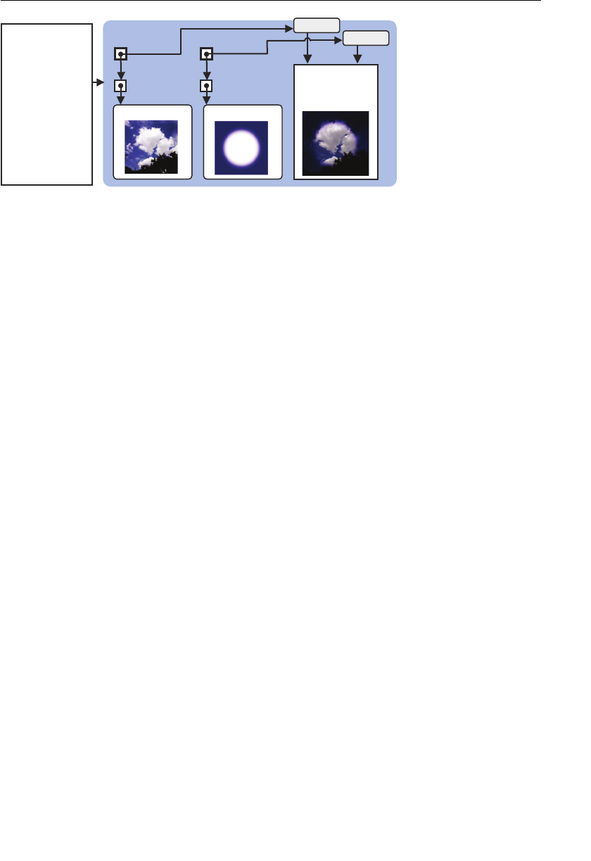
ptg11539634

Pasting Multiple Textures to a Shape 189

…1ERUTXET.lg0ERUTXET.lg

D2_ERUTXET.lg

D2_ERUTXETlg

tpircSavaJ

…LGbeWteg=lgrav

…

{)(niamnoitcnuf

0relpmaS_u

1relpmaS_u

;)…(i1mrofinu.lg

;)…(i1mrofinu.lg tcejbOerutxeT

tnemgarF

redahS

tcejbOerutxeT

Figure 5.37 Internal state of WebGL when handling two texture images

Finally, the program invokes the vertex shader after checking whether both texture images

are available at line 165 using

g_texUnit0 and g_texUnit1 . The images are then combined

as they are mapped to the shape, resulting in the screenshot in Figure 5.34 .

Summary

In this chapter, you ventured deep into the WebGL world. At this stage you have acquired

all the basic skills needed to use WebGL to deal with 2D geometric shapes and are ready

for the next step: 3D objects. Fortunately, when you deal with 3D objects instead of 2D

shapes, the way you use shaders is surprisingly similar, so you can quickly apply all the

knowledge you’ve learned so far.

The rest of this book focuses mainly on covering the techniques necessary for managing

3D objects. However, before introducing you to the 3D world, the next chapter will take a

brief tour of the OpenGL ES shading language (GLSL ES), covering some features and func-

tionality that have been only touched on in the chapters so far.

ptg11539634

This page intentionally left blank

ptg11539634

Chapter 6

The OpenGL ES Shading Language (GLSL ES)

This chapter takes a break from examining WebGL sample programs and explains the essential

features of the OpenGL ES Shading Language (GLSL ES) in detail.

As you have seen, shaders are the core mechanism within WebGL for constructing 3DCG

programs, and GLSL ES is the dedicated programming language for writing those shader

programs. This chapter covers:

• Data, variables, and variable types

• Vector, matrix, structure, array, and sampler types

• Operators, control flow, and functions

• Attributes, uniform, and varying variables

• Precision qualifiers

• Preprocessor and directives

By the end of this chapter, you will have a good understanding of GLSL ES and how to use it to

write a variety of shaders. This knowledge will help you tackle the more complex 3D manipula-

tions introduced in Chapters 7 through 9 . Note that language specifications can be quite dry, and

for some of you, this may be more detail than you need. If so, it’s safe to skip this chapter and

use it as a reference when you look at the examples in the rest of the book.

Recap of Basic Shader Programs

As you can see from Listings 6.1 and 6.2 , you can construct shader programs in a similar manner

to constructing programs using the C programming language.

ptg11539634

CHAPTER 6 The OpenGL ES Shading Language (GLSL ES)

192

Listing 6.1 Example of a Simple Vertex Shader

// Vertex shader

attribute vec4 a_Position;

attribute vec4 a_Color;

uniform mat4 u_MvpMatrix;

varying vec4 v_Color;

void main() {

gl_Position = u_MvpMatrix * a_Position;

v_Color = a_Color;

}

Variables are declared at the beginning of the code, and then the main() routine defines

the entry point for the program.

Listing 6.2 Example of a Simple Fragment Shader

// Fragment shader

#ifdef GLSL_ES

precision mediump float;

#endif

varying vec4 v_Color;

void main() {

gl_FragColor = v_Color;

}

The version of GLSL ES dealt with in this chapter is 1.00. However, you should note that

WebGL does not support all features defined in GLSL ES 1.00

1 ; rather, it supports a subset

of 1.00 with core features needed for WebGL.

Overview of GLSL ES

The GLSL ES programming language was developed from the OpenGL Shading Language

(GLSL) by reducing or simplifying functionality, assuming that the target platforms were

consumer electronics or embedded devices such as smart phones and game consoles.

A prime goal was to allow hardware manufacturers to simplify the hardware needed to

execute GLSL ES programs. This had two key benefits: reducing power consumption by

devices and, perhaps more importantly, reducing manufacturing costs.

GLSL ES supports a limited (and partially extended) version of the C language syntax.

Therefore, if you are familiar with the C language, you’ll find it easy to understand

GLSL ES. Additionally, the shading language is beginning to be used for general-purpose

processing such as image processing and numerical computation (so called GPGPU),

meaning that GLSL ES has an increasingly wide application domain, thus increasing the

benefits of studying the language.

1 http://www.khronos.org/registry/gles/specs/2.0/GLSL_ES_Speci cation_1.0.17.pdf

ptg11539634

Hello Shader! 193

Hello Shader!

By tradition, most programming books begin with a “Hello World!” example, or in our

case the corresponding shader program. However, because you have already seen several

shader programs in previous chapters, let’s skip that and take a look at the basics of GLSL

ES, using Listing 6.1 and Listing 6.2 shown earlier.

Basics

Like many programming languages, you need to pay attention to the following two items

when you write shader programs using GLSL ES:

• The programs are case-sensitive ( marina and Marina are different).

• A semicolon (;) must be specified at the end of each command.

Order of Execution

Once a JavaScript program is loaded, program lines are executed in the order in which

they were written—sequentially starting from the first program line. However, like C,

shader programs are executed from the function

main() and therefore must have one (and

only one)

main() function that cannot have any parameters. Looking back, you can see

that each shader program shown in Listing 6.1 and Listing 6.2 defines a single

main() .

You must prepend the keyword void to main() , which indicates that the function has

no return value. (See the section “Functions” later in this chapter.) This is different from

JavaScript, where you can define a function using the keyword

function , and you don’t

have to worry whether the function returns a value. In GLSL ES, if the function returns a

value, you must specify its data type in front of the function name, or if it doesn’t return

a value, specify

void so that the system doesn’t expect a return value.

Comments

As with JavaScript, you can write comments in your shader program, and in fact use the

same syntax as JavaScript. So, the following two types of comment are supported:

• // characters followed by any sequence of characters up to the end of line:

int kp = 496; // kp is a Kaprekar number

• /* characters, followed by any sequence of characters (including new lines), followed

by the */ characters:

/* I have a day off today.

I want to take a day off tomorrow.

ptg11539634

CHAPTER 6 The OpenGL ES Shading Language (GLSL ES)

194

Data (Numerical and Boolean Values)

GLSL ES supports only two data types:

• Numerical value: GLSL ES supports integer numbers (for example, 0, 1, 2) and float-

ing point numbers (for example, 3.14, 29.98, 0.23571). Numbers without a decimal

point (.) are treated as integer numbers, and those with a decimal point are treated

as floating point numbers.

• Boolean value: GLSL ES supports true and false as boolean constants.

GLSL ES does not support character strings, which may initially seem strange but makes

sense for a 3D graphics language.

Variables

As you have seen in the previous chapters, you can use any variable names you want as

long as the name follows the basic naming rules:

• The character set for variables names contains only the letters a–z, A–Z, the under-

score (_), and the numbers 0–9.

• Numbers are not allowed to be used as the first character of variable names.

• The keywords shown in Table 6.1 and the reserved keywords shown in Table 6.2 are

not allowed to be used as variable names. However, you can use them as part of the

variable name, so the variable name

if will result in error, but iffy will not.

• Variable names starting with gl_ , webgl_ , or _webgl_ are reserved for use by OpenGL

ES. No user-defined variable names may begin with them.

Table 6.1 Keywords Used in GLSL ES

attribute bool break bvec2 bvec3 bvec4

const continue discard do else false

float for highp if in inout

Int invariant ivec2 ivec3 ivec4 lowp

mat2 mat3 mat4 medium out precision

return sampler2D samplerCube struct true uniform

varying vec2 vec3 vec4 void while

ptg11539634

Basic Types 195

Table 6.2 Reserved Keywords for Future Version of GLSL ES

asm cast class default

double dvec2 dvec3 dvec4

enum extern external fixed

flat fvec2 fvec3 fvec4

goto half hvec2 hvec3

hvec4 inline input interface

long namespace noinline output

packed public sampler1D sampler1DShadow

sampler2DRect sampler2DRectShadow sampler2DShadow sampler3D

sampler3DRect short sizeof static

superp switch template this

typedef union unsigned using

volatile

GLSL ES Is a Type Sensitive Language

GLSL ES does not require the use of var to declare variables, but it does require you to

specify the type of data a variable will contain. As you have seen in the sample programs,

you declare variables using the form

such as vec4 a_Position .

As discussed, when you define a function like main() , you must also specify the data type

of the return value of the function. Equally, the type of data on the left side of the assign-

ment operation (=) and that of data on the right side must have the same type; otherwise,

it will result in an error.

For these reasons, GLSL ES is called a type sensitive language , meaning that it belongs to

a class of languages that require you to specify and pay attention to types.

Basic Types

GLSL ES supports the basic data types shown in Table 6.3 .

ptg11539634

CHAPTER 6 The OpenGL ES Shading Language (GLSL ES)

196

Table 6.3 GLSL Basic Types

Type Description

float The data type for a single floating point number. It indicates the variable will contain

a single floating point number.

int The data type for a single integer number. It indicates the variable will contain a

single integer number.

bool The data type for a boolean value. It indicates the variable will contain a boolean

value.

Specifying the data type for variables allows the WebGL system to check errors in advance

and process the program efficiently. The following are examples of variable declarations

using basic types.

float klimt; // The variable will contain a single floating number

int utrillo; // The variable will contain a single integer number

bool doga; // The variable will contain a single boolean value

Assignment and Type Conversion

Assignments of values to variables are performed using the assignment operator ( = ). As

mentioned, because GLSL ES is a type-sensitive language, if the data type of the left-side

variable is not equal to that of the assigned data (or variable), it will result in an error:

int i = 8; // OK

float f1 = 8; // Error

float f2 = 8.0; // OK

float f3 = 8.0f; // Error: Expressions like 8.0f used in C are not allowed.

Semantically, 8 and 8.0 are the same values. However, when you assign 8 to a floating

point variable

f1 , it will result in an error. In this case, you would see the following error

message:

failed to compile shader: ERROR: 0:11: ‘=’ : cannot convert from ‘const mediump int’

to ‘float’.

If you want to assign an integer number to a floating point variable, you need to convert

the integer number to a floating point number. This conversion is called type conversion .

To convert an integer into a floating point number, you can use the built-in function

float() , as follows:

int i = 8;

float f1 = float(i); // 8 is converted to 8.0 and assigned to f1

float f2 = float(8); // equivalent to the above operation

ptg11539634

Basic Types 197

GLSL ES supports a number of other built-in functions for type conversion, which are

shown in Table 6.4 .

Table 6.4 The Built-In Functions for Type Conversion

Conversion Function Description

To an integer

number

int(float) The fractional part of the floating-point value is

dropped (for example, 3.14 → 3).

int(bool) true is converted to 1, or false is converted to 0.

To a floating

point number

float(int) The integer number is converted to a floating point

number (for example, 8 → 8.0).

float(bool) true is converted to 1.0, or false is converted to

0.0.

To a boolean

value

bool(int) 0 is converted to false , or non-zero values are

converted to

true .

bool(float) 0.0 is converted to false , or non-zero values are

converted to

true .

Operations

The operators applicable to the basic types are similar to those in JavaScript and are shown

in Table 6.5 .

Table 6.5 The Operators Available for the Basic Types

Operator Operation Applicable Data Type

— Negation (for example,

for specifying a negative

number)

int or float .

* Multiplication int or float . The data type of the

result of the operation is the same

as operands.

/ Division

+ Addition

— Subtraction

++ Increment (postfix and

prefix)

int or float . The data type of the

result of the operation is the same

as operands.

— Decrement (postfix and

prefix)

= Assignment int , float , or bool

+= -= *= /= Arithmetic assignment int or float .

ptg11539634

CHAPTER 6 The OpenGL ES Shading Language (GLSL ES)

198

Operator Operation Applicable Data Type

< > <= >= Comparison int or float .

== != Comparison (equality) int , float , or bool .

! Not bool or an expression that results

bool [1].

&& Logical and

|| Logical inclusive or

^^ Logical exclusive or [2]

condition?

expression1: expression2

Ternary selection condition is

bool or an expression

that results in

bool . Data types

other than array can be used in

expression1 and expression2 .

[1] The second operand in a logical and ( && ) operation is evaluated if and only if the first operand

evaluates to true . The second operand in a logical or ( || ) operation is evaluated if and only if the

first operand evaluates to false .

[2] If either the left-side condition or the right-side one is true , the result is true . If both sides are

true , the result is false .

The followings are examples of basic operations:

int i1 = 954, i2 = 459;

int kp = i1 — i2; // 495 is assigned to kp.

float f = float(kp) + 5.5; // 500.5 is assigned to f.

Vector Types and Matrix Types

GLSL ES supports vector and matrix data types which, as you have seen, are useful when

dealing with computer graphics. Both these types contain multiple data elements. A

vector type, which arranges data in a list, is useful for representing vertex coordinates or

color data. A matrix arranges data in an array and is useful for representing transformation

matrices. Figure 6.1 shows an example of both types.

)(

351173

704

173

Figure 6.1 A vector and a matrix

GLSL ES supports a variety of vector or matrix types, as shown in Table 6.6 .

ptg11539634

Vector Types and Matrix Types 199

Table 6.6 Vector Types and Matrix Types

Category Types in GLSL ES Description

Vector vec2 , vec3 , vec4 The data types for 2, 3, and 4 component vectors of

floating point numbers

ivec2 , ivec3 , ivec4 The data types for 2, 3, and 4 component vectors of

integer numbers

bvec2 , bvec3 , bvec4 The data types for 2, 3, and 4 component vectors of

boolean values

Matrix mat2 , mat3 , mat4 The data type for 2×2, 3×3, and 4×4 matrix of floating

point numbers (with 4, 9, and 16 elements, respec-

tively)

The following examples show the use of the vector and matrix types:

vec3 position; // variable for 3-component vector of float

// For example: (10.0, 20.0, 30.0)

ivec2 offset; // variable for 2-component vector of integer

// For example: (10, 20)

mat4 mvpMatrix; // the variable for 4×4 matrix of float

Assignments and Constructors

Assignment of data to variables of the type vector or matrix is performed using the =

operator. Remember that the type of data on the left side of the assignment operation and

that of the data/variable on the right side must be the same. In addition, the number of

elements on the left side of the assignment operation must be equal to that of the data/

variable on the right side. To illustrate that, the following example will result in an error:

vec4 position = 1.0; // vec4 variable requires four floating point numbers

In this case, because a vec4 variable requires four floating point numbers, you need to pass

four floating numbers in some way. A solution is to use the built-in functions with the

same name of the data type so; for example, in the case of

vec4 , you can use the construc-

tor

vec4() . (See Chapter 2 , “Your First Step with WebGL.”) For example, to assign 1.0, 2.0,

3.0, and 4.0 to a variable of type

vec4 , you can use vec4() to bundle them into a single

data element as follows:

vec4 position = vec4(1.0, 2.0, 3.0, 4.0);

Functions for making a value of the specified data type are called constructor functions ,

and the name of the constructor is always identical to that of the data type.

ptg11539634

CHAPTER 6 The OpenGL ES Shading Language (GLSL ES)

200

Vector Constructors

Vectors are critical in GLSL ES so, as you’d imagine, there are multiple ways to specify

arguments to a vector constructor. For example:

vec3 v3 = vec3(1.0, 0.0, 0.5); // sets v3 to(1.0, 0.0, 0.5)

vec2 v2 = vec2(v3); // sets v2 to (1.0, 0.0) using the 1st and 2nd elements of v3

vec4 v4 = vec4(1.0); // sets v4 to (1.0, 1.0, 1.0, 1.0)

In the second example, the constructor ignores the third element of v3 , and only the

first and second elements of

v3 are used to create the new vector. Similarly, in the third

example, if a single value is specified to a vector constructor, the value is used to initialize

all components of the constructed vector. However, if more than one value is specified

to a vector constructor but the number of the values is less than the number of elements

required by the constructor, it will result in an error.

Finally, a vector can be constructed from multiple vectors:

vec4 v4b = vec4(v2, v4); // sets (1.0, 0.0, 1.0, 1.0) to v4b

The rule here is that the vector is filled with values from the first vector (v2), and then

any missing values are supplied by the second vector (v4).

Matrix Constructors

Constructors are also available for matrices and operate in a similar manner to vector

constructors. However, you should make sure the order of elements stored in a matrix is

in a column major order. (See Figure 3.27 for more details of “column-major order.”) The

following examples show different ways of using the matrix constructor:

• If multiple values are specified to a matrix constructor, a matrix is constructed using

them in column major order:

mat4 m4 = mat4 ( 1.0, 2.0, 3.0, 4.0,

5.0, 6.0, 7.0, 8.0,

9.0, 10.0, 11.0, 12.0,

13.0, 14.0, 15.0, 16.0 );

• If multiple vectors are specified to a matrix constructor, a matrix is constructed using

the elements of each vector in column major order:

// two vec2 are used to construct a mat2

vec2 v2_1 = vec2(1.0, 3.0);

vec2 v2_2 = vec2(2.0, 4.0);

mat2 m2_1 = mat2(v2_1, v2_2); // 1.0 2.0

// 3.0 4.0

// vec4 is used to construct mat2

vec4 v4 = vec4(1.0, 3.0, 2.0, 4.0);

⎡

⎣

⎢

⎤

⎦

⎥

1.0 5.0 9.0 13.0

2.0 6.0 10.0 14.0

3.0 7.0 11.0 15.0

4.0 8.0 12.0 16.0

ptg11539634

Vector Types and Matrix Types 201

mat2 m2_2 = mat2(v4); // 1.0 2.0

// 3.4 4.0

• If multiple values and multiple vectors are specified to a matrix constructor, a matrix

is constructed using them in column major order:

// Two floating point numbers and vec2 are used to construct a mat2

mat2 m2 = mat2(1.0, 3.0, v2_2); // 1.0 2.0

// 3.0 4.0

• If a single value is specified to a matrix constructor, a matrix is constructed using the

value as its diagonal elements:

mat4 m4 = mat4(1.0); // 1.0 0.0 0.0 0.0

// 0.0 1.0 0.0 0.0

// 0.0 0.0 1.0 0.0

// 0.0 0.0 0.0 1.0

Similar to a vector constructor, if an insufficient number of values is specified to the

constructor (but more than one), it will result in an error.

mat4 m4 = mat4(1.0, 2.0, 3.0); // Error. mat4 requires 16 elements.

Access to Components

To access the components in a vector or matrix, you can use the operators . and [] , as

shown in the following subsections.

The . Operator

An individual component in a vector can be accessed by the variable name followed by

period (.) and then the component name, as shown in Table 6.7 .

Table 6.7 Component Names

Category Description

x , y , z , w Useful for accessing vertex coordinates.

r , g , b , a Useful for accessing colors.

s , t , p , q Useful for accessing texture coordinates. (Note that this book uses only s and

t . p is used instead of r because r is used for colors.)

Because vectors are used for storing various types of data such as vertex coordinates,

colors, and texture coordinates, three types of component names are supported to increase

ptg11539634

CHAPTER 6 The OpenGL ES Shading Language (GLSL ES)

202

the readability of programs. However, any of the component names x , r , or s accesses the

first component; any of

y , g , or t accesses the second one; and so on, so you can use them

interchangeably if you prefer. For example:

vec3 v3 = vec3(1.0, 2.0, 3.0); // sets v3 to(1.0, 2.0, 3.0)

float f;

f = v3.x; // sets f to 1.0

f = v3.y; // sets f to 2.0

f = v3.z; // sets f to 3.0

f = v3.r; // sets f to 1.0

f = v3.s; // sets f to 1.0

As you can see from the comments of these examples, x , r , and s have different names

but always access the first component. Attempting to access a component beyond the

number of components in the vector will result in an error:

f = v3.w; // w requires access to the fourth element, which doesn’t exist.

Multiple components can be selected by appending their names (from the same name set)

after the period (.). This is known as swizzling . In the following example,

x , y , z , and w

will be used, but other sets of component names have the same effect:

vec2 v2;

v2 = v3.xy; // sets v2 to (1.0, 2.0)

v2 = v3.yz; // sets v2 to (2.0, 3.0). Any component can be omitted

v2 = v3.xz; // sets v2 to (1.0, 3.0). You can skip any component.

v2 = v3.yx; // sets v2 to (2.0, 1.0). You can reverse the order.

v2 = v3.xx; // sets v2 to (1.0, 1.0). You can repeat any component.

vec3 v3a;

v3a = v3.zyx; // sets v3a to (3.0, 2.0, 1.0). You can use all names.

The component name can also be used in the left-side expression of an assignment opera-

tor (

= ):

vec4 position = vec4(1.0, 2.0, 3.0, 4.0);

position.xw = vec2(5.0, 6.0); // position = (5.0, 2.0, 3.0, 6.0)

Remember, the component names must come from the same set so, for example, v3.was is

not allowed.

ptg11539634

Vector Types and Matrix Types 203

The [ ] Operator

In addition to the

. operator, the components of a vector or a matrix can be accessed

using the array indexing operator

[] . Note that the elements in a matrix are also read out

in column major order. Just like JavaScript, the index starts from 0, so applying

[0] to a

matrix selects the first column in the matrix,

[1] selects the second one, [2] selects the

third one, and so on. The following shows an example:

mat4 m4 = mat4 ( 1.0, 2.0, 3.0, 4.0,

5.0, 6.0, 7.0, 8.0,

9.0, 10.0, 11.0, 12.0,

13.0, 14.0, 15.0, 16.0);

vec4 v4 = m4[0]; // Retrieve the 1st column from m4: (1.0, 2.0, 3.0, 4.0)

In addition, two [] operators can be used to select a column and then a row of a matrix:

float m23 = m4[1][2]; // sets m23 to the third component of the second

// column of m4 (7.0).

A component name can be used to select a component in conjunction with the [] opera-

tor, as follows:

float m32 = m4[2].y; // sets m32 to the second component of the third

// column of m4 (10.0).

One restriction is that only a constant index can be specified as the index number in the

[] operator. The constant index is defined as

• A integral literal value (for example, 0 or 1)

• A global or local variable qualified as const , excluding function parameters (see the

section “const Variables”)

• Loop indices (see the section “Conditional Control Flow and Iteration”)

• Expressions composed from any of the preceding

The following examples use the type

int constant index:

const int index = 0; // «const» keyword specifies the variable is a

// read-only variable.

vec4 v4a = m4[index]; // is the same as m4[0]

The following example uses an expression composed of constant indices as an index.

vec4 v4b = m4[index + 1]; // is the same as m4[1]

ptg11539634

CHAPTER 6 The OpenGL ES Shading Language (GLSL ES)

204

Remember, you cannot use an int variable without the const qualifier as an index

because it is not a constant index (unless it is a loop index):

int index2 = 0;

vec4 v4c = m4[index2]; // Error: because index2 is not a constant index.

Operations

You can apply the operators shown in Table 6.8 to a vector or a matrix. These operators

are similar to the operators for basic types. Note that the only comparative operators avail-

able for a vector and matrix are

== and != . The < , > , <=, and >= operators cannot be used

for comparisons of vectors or matrices. In such cases, you can use built-in functions such

lessThan() . (See Appendix B , “Built-In Functions of GLSL ES 1.0.”)

Table 6.8 The Operators Available for a Vector and a Matrix

Operators Operation Applicable Data Types

* Multiplication vec[234] and mat[234] . The opera-

tions on

vec[234] and mat[234] will be

explained below.

The data type of the result of operation is

the same as the operands.

/ Division

+ Addition

— Subtraction

++ Increment (postfix and prefix) vec[234] and mat[234] . The data type of

the result of this operation is the same as

the operands.

— Decrement (postfix and prefix)

= Assignment vec[234] and mat[234] .

+=, -=,

*=, /=

Arithmetic assignment vec[234] and mat[234] .

==, != Comparison vec[234] and mat[234] . With == , if all

components of the operands are equal,

the result is

true . For != , if any of compo-

nents of the operands are not equal, then

the result is

true [1].

[1] If you want component-wise equality, you can use the built-in function equal() or

notEqual(). (See Appendix B .)

Note that when an arithmetic operator operates on a vector or a matrix, it is operating

independently on each component of the vector or matrix in component-wise order.

Examples

The following examples show frequently used cases. In the examples, we assume that the

types of variables are defined as follows:

ptg11539634

Vector Types and Matrix Types 205

vec3 v3a, v3b, v3c;

mat3 m3a, m3b, m3c;

float f;

Operations on a Vector and Floating Point Number

An example showing the use of the

+ operator:

// The following example uses the + operator, but the -, *, and /

// operators also have the same effect.

v3b = v3a + f; // v3b.x = v3a.x + f;

// v3b.y = v3a.y + f;

// v3b.z = v3a.z + f;

For example, v3a = vec3(1.0, 2.0, 3.0) and f = 1.0 will result in v3b=(2.0, 3.0,

4.0) .

Operations on Vectors

These operators operate on each component of a vector:

// The following example uses the + operator, but the -, *, and /

// operators also have the same effect.

v3c = v3a + v3b; // v3a.x + v3b.x;

// v3a.y + v3b.y;

// v3a.z + v3b.z;

For example, v3a = vec3(1.0, 2.0, 3.0) and v3b = vec3(4.0, 5.0, 6.0) will result in

v3c=(5.0, 7.0, 9.0) .

Operations on a Matrix and a Floating Point Number

These operators operate on each component of the matrix:

// The following example uses the + operator, but the -, *, and /

// operators also have the same effect.

m3b = m3a * f; // m3b[0].x = m3a[0].x * f; m3b[0].y = m3a[0].y * f;

// m3b[0].z = m3a[0].z * f;

// m3b[1].x = m3a[1].x * f; m3b[1].y = m3a[1].y * f;

// m3b[1].z = m3a[1].z * f;

// m3b[2].x = m3a[2].x * f; m3b[2].y = m3a[2].y * f;

// m3b[2].z = m3a[2].z * f;

Multiplication of a Matrix and a Vector

For multiplication, the result is the sum of products of each element in a matrix and

vector. This result is the same as Equation 3.5 that you saw back in Chapter 3 , “Drawing

and Transforming Triangles”:

ptg11539634

CHAPTER 6 The OpenGL ES Shading Language (GLSL ES)

206

v3b = m3a * v3a; // v3b.x = m3a[0].x * v3a.x + m3a[1].x * v3a.y

// + m3a[2].x * v3a.z;

// v3b.y = m3a[0].y * v3a.x + m3a[1].y * v3a.y

// + m3a[2].y * v3a.z;

// v3b.z = m3a[0].z * v3a.x + m3a[1].z * v3a.y

// + m3a[2].z * v3a.z;

Multiplication of a Vector and a Matrix

Multiplication of a vector and a matrix is possible, as you can see from the following

expressions. Note that this result is different from that when multiplying a matrix by a

vector:

v3b = v3a * m3a; // v3b.x = v3a.x * m3a[0].x + v3a.y * m3a[0].y

// + v3a.z * m3a[0].z;

// v3b.y = v3a.x * m3a[1].x + v3a.y * m3a[1].y

// + v3a.z * m3a[1].z;

// v3b.z = v3a.x * m3a[2].x + v3a.y * m3a[2].y

// + v3a.z * m3a[2].z;

Multiplication of Matrices

This is the same as Equation 4.4 in Chapter 4 , “More Transformations and Basic

Animation”:

m3c = m3a * m3b; // m3c[0].x = m3a[0].x * m3b[0].x + m3a[1].x * m3b[0].y

// + m3a[2].x * m3b[0].z;

// m3c[1].x = m3a[0].x * m3b[1].x + m3a[1].x * m3b[1].y

// + m3a[2].x * m3b[1].z;

// m3c[2].x = m3a[0].x * m3b[2].x + m3a[1].x * m3b[2].y

// + m3a[2].x * m3b[2].z;

// m3c[0].y = m3a[0].y * m3b[0].x + m3a[1].y * m3b[0].y

// + m3a[2].y * m3b[0].z;

// m3c[1].y = m3a[0].y * m3b[1].x + m3a[1].y * m3b[1].y

// + m3a[2].y * m3b[1].z;

// m3c[2].y = m3a[0].y * m3b[2].x + m3a[1].y * m3b[2].y

// + m3a[2].y * m3b[2].z;

// m3c[0].z = m3a[0].z * m3b[0].x + m3a[1].z * m3b[0].y

// + m3a[2].z * m3b[0].z;

// m3c[1].z = m3a[0].z * m3b[1].x + m3a[1].z * m3b[1].y

// + m3a[2].z * m3b[1].z;

// m3c[2].z = m3a[0].z * m3b[2].x + m3a[1].z * m3b[2].y

// + m3a[2].z * m3b[2].z;

ptg11539634

Structures 207

Structures

GLSL ES also supports user-defined types, called structure s, which aggregate other already

defined types using the keyword

struct . For example:

struct light { // defines the structure «light»

vec4 color;

vec3 position;

}

light l1, l2; // declares variable «l1» and «l2» of the type «light»

This example defines the new structure type light that consists of two members: the vari-

able

color and position . Then two variables l1 and l2 of type light are declared after the

definition. Unlike C, the

typedef keyword is not necessary because, by default, the name

of the structure becomes the name of the type.

In addition, as a convenience, variables of the new type can be declared with the defini-

tion of the structure, as follows:

struct light { // declares structure and its variable all together

vec4 color; // color of a light

vec3 position; // position of a light

} l1; // variable «l1» of the structure

Assignments and Constructors

Structures support the standard constructor, which has the same name as the structure.

The arguments to the constructor must be in the same order and of the same type as they

were declared in the structure. Figure 6.2 shows an example.

;))0.0,0.3,0.8(3 cev,)0.1,0.0,0.1,0.0(4cev(thgil=1l

roloc noitisop

Figure 6.2 A constructor of structure

Access to Members

Each member of a structure can be accessed by appending the variable name with a period

(.) and then the member name. For example:

vec4 color = l1.color;

vec3 position = l1.position;

ptg11539634

CHAPTER 6 The OpenGL ES Shading Language (GLSL ES)

208

Operations

For each member in the structure, you can use any operators allowed for that member’s

type. However, the operators allowed for the structure itself are only the assignment (

= )

and comparative operators (

== and != ); see Table 6.9.

Table 6.9 The Operators Available for a Structure

Operator Operation Description

= Assignment The assignment and comparison operators are not allowed for

the structures that contain arrays or sampler types

==,!= Comparison

When using the

== operator, the result is true if, and only if, all the members are

component-wise equal. When using the !=, the result is

false if one of the members is

not component-wise equal.

Arrays

GLSL ES arrays have a similar form to the array in JavaScript, with only one-dimensional

arrays being supported. Unlike arrays in JavaScript, the

new operator is not necessary to

create arrays, and methods such as

push() and pop() are not supported. The arrays can be

declared by a name followed by brackets (

[] ) enclosing their sizes. For example:

float floatArray[4]; // declares an array consisting of four floats

vec4 vec4Array[2]; // declares an array consisting of two vec4s

The array size must be specified as an integral constant expression greater than zero

where the integral constant expression is defined as follows:

• A numerical value (for example, 0 or 1)

• A global or local variable qualified as const , excluding function parameters (see the

section “const Variables”)

• Expressions composed of both of the above

Therefore, the following will result in an error:

int size = 4;

vec4 vec4Array[size]; // Error. If you declare «const int size = 4;»

// it will not result in an error

Note that arrays cannot be qualified as const .

ptg11539634

Samplers 209

Array elements can be accessed using the array indexing operator ([]). Note that, like C,

the index starts from 0. For example, the third element of the float Array defined earlier

can be accessed as follows:

float f = floatArray[2];

Only an integral constant expression or uniform variable (see the section “Uniform

Variables”) can be used as an index of an array. In addition, unlike JavaScript or C, an

array cannot be initialized at declaration time. So each element of the array must be

initialized explicitly as follows:

vec4Array[0] = vec4(4.0, 3.0, 6.0, 1.0);

vec4Array[1] = vec4(3.0, 2.0, 0.0, 1.0);

Arrays support only [] operators. However, elements in an array do support the standard

operators available for their type. For example, the following operator can be applied to

the elements of

floatArray or vec4Array :

// multiplies the second element of floatArray by 3.14

float f = floatArray[1] * 3.14;

// multiplies the first element of vec4Array by vec4(1.0, 2.0, 3.0, 4.0);

vec4 v4 = vec4Array[0] * vec4(1.0, 2.0, 3.0, 4.0);

Samplers

GLSL ES supports a dedicated type called sampler for accessing textures. (See Chapter 5 ,

“Using Colors and Texture Images.”) Two types of samplers are available:

sampler2D and

samplerCube . Variables of the sampler type can be used only as a uniform variable (see

the section “Uniform Variables”) or an argument of the functions that can access textures

such as

texture2D() . (See Appendix B .) For example:

uniform sampler2D u_Sampler;

In addition, the only value that can be assigned to the variable is a texture unit number,

and you must use the WebGL method

gl.uniform1i() to set the value. For example,

TexturedQuad.js in Chapter 5 uses gl.uniform1i(u_Sampler, 0) to pass the texture unit

0 to the shader.

Variables of type

sampler are not allowed to be operands in any expressions other than = ,

== , and != .

Unlike other types explained in the previous sections, the number of sampler type vari-

ables is limited depending on the shader type (see Table 6.10 ). In the table, the keyword

mediump is a precision qualifier. (This qualifier is explained in detail in the section

“Precision Qualifiers,” toward the end of this chapter.)

ptg11539634

CHAPTER 6 The OpenGL ES Shading Language (GLSL ES)

210

Table 6.10 Minimum Number of Variables of the Sampler Type

Shaders that Use the

Variable

Built-In Constants Representing the

Maximum Number

Minimum Number

Vertex shader

const mediump int

gl_MaxVertexTextureImageUnits

Fragment shader

const mediump int

gl_MaxTextureImageUnits

Precedence of Operators

Operator precedence is shown in Table 6.11 . Note the table contains several operators that

are not explained in this book but are included for reference.

Table 6.11 The Precedence of Operators

Precedence Operators

1 parenthetical grouping (())

2 function calls, constructors (()), array indexing ([]), period (.)

3 increment/decrement (++, —), negate (-), inverse(~) , not(!)

4 multiplication (*), division (/), remainder (%)

5 addition (+), subtraction (-)

6 bit-wise shift (<<, >>)

7 comparative operators (<, <=, >=, >)

8 equality (==, !=)

9 bit-wise and (&)

10 bit-wise exclusive or (^)

11 bit-wise or (|)

12 and (&&)

13 exclusive or (^^)

14 or (||)

15 ternary selection (?

16 assignment (=), arithmetic assignments (+=, -=, *=, /=, %=,

<<=, >>=, &=, ^=, |= )

17 sequence(,)

Bold font indicates operators reserved for future versions of GLSL.

ptg11539634

Conditional Control Flow and Iteration 211

Conditional Control Flow and Iteration

Conditional control flow and iteration in the shading language are almost the same as in

JavaScript or C.

if Statement and if-else Statement

A conditional control flow can use either if or if-else . An if-else statement follows the

pattern shown here:

if ( conditional-expression1 ) {

commands here are executed if conditional-expression1 is true.

} else if ( conditional-expression2 ) {

commands here are executed if conditional-expression1 is false but conditional-

expression2 is true.

} else {

commands here are executed if conditional-expression1 is false and conditional-

expression2 is false.

}

The following shows a code example using the if-else statement:

if(distance < 0.5) {

gl_FragColor = vec4(1.0, 0.0, 0.0, 1.0); // red

} else {

gl_FragColor = vec4(0.0, 1.0, 0.0, 1.0); // green

}

As shown in this example, the conditional expression in the if or if-else statement must

be either a boolean value or an expression that becomes a boolean value. Boolean vector

types, such as

bvec2 , are not allowed in the conditional expression.

Switch statement are not allowed, and you should note that usage of the if or if-else

statement will slow down the shaders.

for Statement

The for statement can be used as follows:

for ( for-init-statement ; conditional-expression ; loop-index-expression ) {

the commands which you want to execute repeatedly .

}

For example:

for (int i = 0; i < 3; i++) {

sum += i;

}

ptg11539634

CHAPTER 6 The OpenGL ES Shading Language (GLSL ES)

212

Note that the loop index ( i in the preceding example) of the for statement can be

declared only in the for-init-statement . The conditional-expression can be omitted, and an

empty condition becomes true. The

for statement has the following restrictions:

• Only a single loop index is allowed. The loop index must have the type int or

float .

• loop-index-expression must have one of the following forms (supposing that i is a

loop index):

i++ , i— , i+= constant-expression , i-= constant-expression

• conditional-expression is a comparison between a loop index and an integral constant

expression. (See the section “Array.”)

• Within the body of the loop, the loop index cannot be assigned.

These limitations are in place so that the compiler can perform inline expansion of for

statements.

continue, break, discard Statements

Just like JavaScript or C, continue and break statements are allowed only within a for

statement and are generally used within

if statements:

continue skips the remainder of the body of the innermost loop containing the

continue, increases/decreases the loop index, and then moves to the next loop.

break exits the innermost loop containing the break. No further execution of the loop is

done.

The following show examples of the

continue statement:

for (int i = 0; i < 10; i++) {

if (i == {

continue; // skips the remainder of the body of the innermost loop

}

// When i == 8, this line is not executed

}

The following shows an example of the break statement:

for (int i = 0; i < 10; i++) {

if (i == {

break; // exits «for» loop

}

// When i >= 8, this line is not executed.

}

// When i == 8, this line is executed.

ptg11539634

Functions 213

The discard statement is only allowed in fragment shaders and discards the current frag-

ment, abandoning the operation on the current fragment and skipping to the next frag-

ment. The use of

discard will be explained in more detail in the section “Make a Rounded

Point” in Chapter 10 , “Advanced Techniques.”

Functions

In contrast to the way functions are defined in JavaScript, the functions in GLSL ES are

defined in the same manner as in C. For example:

returnType functionName ( type0 arg0 , type1 arg1 , …, typen argn ) {

do some computation

return returnValue ;

}

Argument type s must use one of the data types explained in this chapter, and like main() ,

functions with no arguments are allowed. When the function returns no value, the

return

statement does not need to be included. In this case,

returnType must be void . You can

also specify a structure as the

returnValue , but the structure returned cannot contain an

array.

The following example shows a function to convert an RGBA value into a luminance

value:

float luma (vec4 color) {

float r = color.r;

float g = color.g;

float b = color.b;

return 0.2126 * r + 0.7162 * g + 0.0722 * b;

// The preceding four lines could be rewritten as follows:

// return 0.2126 * color.r + 0.7162 * color.g + 0.0722 * color.b;

}

You can call the function declared above in the same manner as in JavaScript or C by

using its name followed by a list of arguments in parentheses:

attribute vec4 a_Color; // (r, g, b, a) is passed

void main() {

…

float brightness = luma(a_Color);

…

}

Note that an error will result if, when called, argument types do not match the declared

parameter types. For example, the following will result in an error because the type of the

parameter is float, but the caller passes an integer:

ptg11539634

CHAPTER 6 The OpenGL ES Shading Language (GLSL ES)

214

float square(float value) {

return value * value;

}

void main() {

…

float x2 = square(10); // Error: Because 10 is integer. 10.0 is OK.

…

}

As you can see from the previous examples, functions work just like those in JavaScript

or C except that you cannot call the function itself from inside the body of the function

(that is, a recursive call of the function isn’t allowed). For the more technically minded,

this is because the compilers can in-line function calls.

Prototype Declarations

When a function is called before it is defined, it must be declared with a prototype. The

prototype declaration tells WebGL in advance about the types of parameters and the

return value of the function. Note that this is different from JavaScript, which doesn’t

require a prototype. The following is an example of a prototype declaration for

luma() ,

which you saw in the previous section:

float luma(vec4); // a prototype declaration

main() {

…

float brightness = luma(color); // luma() is called before it is defined.

…

}

float luma (vec4 color) {

return 0.2126 * color.r + 0.7162 * color.g + 0.0722 * color.b;

}

Parameter Qualifiers

GLSL ES supports qualifiers for parameters that control the roles of parameters within a

function. They can define that a parameter (1) is to be passed into a function, (2) is to be

passed back out of a function, and (3) is to be passed both into and out of a function. (2)

and (3) can be used just like a pointer in C. These are shown in Table 6.12 .

ptg11539634

Built-In Functions 215

Table 6.12 Parameter Qualifiers

Qualifiers Roles Description

in Passes a value into the function The parameter is passed by value.

Its value can be referred to and

modified in the function. The caller

cannot refer to the modification.

const in Passes a value into the function The parameter is passed by

constant value. Its value can be

referred to but cannot be modified.

out Passes a value out of the function The parameter is passed by refer-

ence. If its value is modified, the

caller can refer to the modification.

inout Passes a value both into/out of the

function

The parameter is passed by refer-

ence, and its value is copied in the

function. Its value can be referred

to and modified in the function. The

caller can also refer to the modifica-

tion.

<none:

default>

Passes a value into the function Same as

in .

For example,

luma() can return the result of its calculation using a parameter qualified by

out instead of a return value, as follows:

void luma2 (in vec3 color, out float brightness) {

brightness = 0.2126 * color.r + 0.7162 * color.g + 0.0722 * color.b;

}

Because the function itself no longer returns a value, the return type of this function is

changed from

float to void . Additionally, the qualifier in , in front of the first parameter,

can be omitted because

in is a default parameter qualifier.

This function can be used as follows:

luma2(color, brightness); // the result is stored into «brightness»

// same as brightness = luma(color)

Built-In Functions

In addition to user-defined functions, GLSL ES supports a number of built-in functions

that perform operations frequently used in computer graphics. Table 6.13 gives an over-

view of the built-in functions in GLSL ES, and you can look at Appendix B for the detailed

definition of each function.

ptg11539634

CHAPTER 6 The OpenGL ES Shading Language (GLSL ES)

216

Table 6.13 Built-In Functions in GLSL ES

Category Built-In Functions

Angle functions

radians (converts degrees to radians), degrees (converts radians to

degrees)

Trigonometry

functions

sin (sine function), cos (cosine function), tan (tangent function), asin

(arc sine function),

acos (arc cosine function), and atan (arc tangent

function)

Exponential

functions

pow (x

y ), exp (natural exponentiation), log (natural logarithm), exp 2 (2

x ),

log2 (base 2 logarithm), sqrt (square root), and inversesqrt (inverse

sqrt )

Common functions abs (absolute value), min (minimum value), max (maximum value), mod

(remainder),

sign (sign of a value), floor (floor function), ceil (ceil

function),

clamp (clamping of a value), mix (linear interpolation), step

(step function),

smoothstep (Hermite interpolation), and fract (frac-

tional part of the argument)

Geometric functions

length (length of a vector), distance (distance between two points),

dot (inner product), cross (outer product), normalize (vector with

length of 1),

reflect (reflection vector), and faceforward (converting

normal when needed to “faceforward”)

Matrix functions

matrixCompMult (component-wise multiplication)

Vector relational

functions

lessThan (component-wise “<”), lessThanEqual (component-wise

“<=”),

greaterThan (component-wise “>”), greaterThanEqual

(component-wise “>=”),

equal (component-wise “==”), notEqual

(component-wise “!=”),

any (true if any component is true), all (true if

all components are true), and

not (component-wise logical complement)

Texture lookup

functions

texture2D (texture lookup in the 2D texture), textureCube (texture

lookup in the cube map texture),

texture2DProj (projective version of

texture2D()), texture2DLod (level of detail version of texture2D()),

textureCubeLod (lod version of textureCube()), and

texture2DProjLod (projective version of texture2DLod())

Global Variables and Local Variables

Just like JavaScript or C, GLSL ES supports both global variables and local variables. Global

variables can be accessed from anywhere in the program, and local variables can be

accessed only from within a limited portion of the program.

In GLSL ES, in a similar manner to JavaScript or C, variables declared “outside” a function

become global variables, and variables declared “inside” a function become local variables.

The local variables can be accessed only from within the function containing them. For

this reason, the attribute, uniform, and varying variables described in the next section

must be declared as global variables because they are accessed from outside the function.

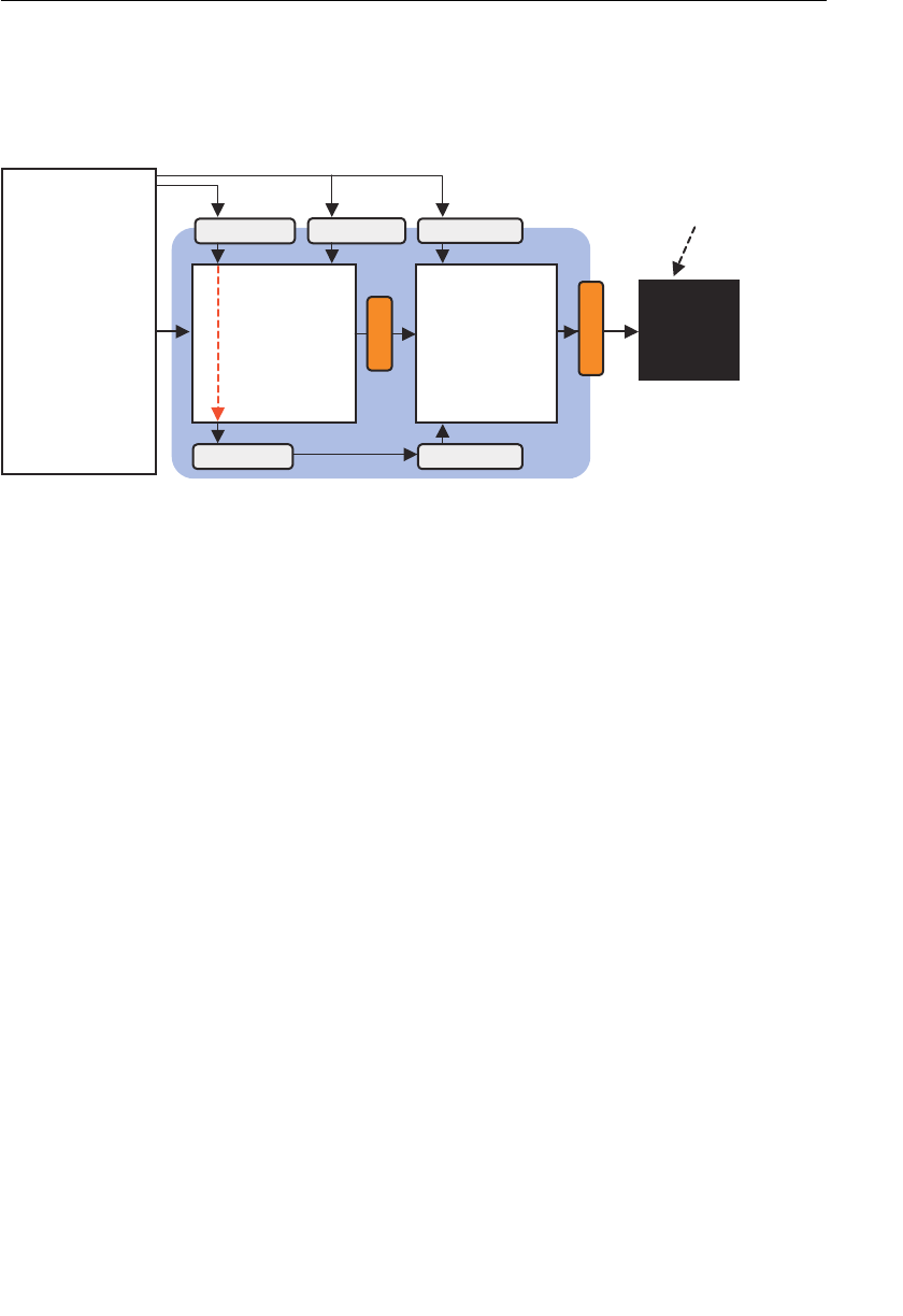
ptg11539634

Storage Qualifiers 217

Storage Qualifiers

As explained in the previous chapters, GLSL ES supports storage qualifiers for attribute,

uniform, and varying variables (see Figure 6.3 ). In addition, a

const qualifier is supported

to specify a constant variable to be used in a shader program.

xetreV

redahS

tnemgarF

redahS

gl_Position

gl_FragColor

elbairavetubirtta elbairavmrofinu

tpircSavaJ

{)(niamnoitcnuf

…LGbeWteg=lgrav

…

;)…(sredahStini

…

}

elbairavgniyrav

elbairavmrofinu

elbairavgniyrav

reffuBroloC

Figure 6.3 Attribute, uniform, and varying variables

const Variables

Unlike JavaScript, GLSL ES supports the const qualifier to specify a constant variable, or

one whose value cannot be modified.

The

const qualifier is specified in front of the variable type, just like an attribute vari-

able. Variables qualified by

const must be initialized at their declaration time; otherwise,

they are unusable because no data can be assigned to them after their declaration. Some

examples include:

const int lightspeed = 299792458; // light speed (m/s)

const vec4 red = vec4(1.0, 0.0, 0.0, 1.0); // red

const mat4 identity = mat4(1.0); // identity matrix

Assigning data to the variable qualified by const will result in an error. For example:

const int lightspeed;

lightspeed = 299792458;

will result in the following error message:

failed to compile shader: ERROR: 0:11: ‘lightspeed’ : variables

with qualifier ‘const’ must be initialized

ERROR: 0:12: ‘assign’: l-value required (can’t modify a const variable)

ptg11539634

CHAPTER 6 The OpenGL ES Shading Language (GLSL ES)

218

Attribute Variables

As you have seen in previous chapters, attribute variables are available only in vertex

shaders. They must be declared as a global variable and are used to pass per-vertex data

to the vertex shader. You should note that it is “per-vertex.” For example, if there are two

vertices, (4.0, 3.0, 6.0) and (8.0, 3.0, 0.0), data for each vertex can be passed to an attribute

variable. However, data for other coordinates, such as (6.0, 3.0, 3.0), which is a halfway

point between the two vertices and not a specified vertex, cannot be passed to the vari-

able. If you want to do that, you need to add the coordinates as a new vertex. Attribute

variables can only be used with the data types

float , vec2 , vec3 , vec4 , mat2 , mat3 , and

mat4 . For example:

attribute vec4 a_Color;

attribute float a_PointSize;

There is an implementation-dependent limit on the number of attribute variables avail-

able, but the minimum number is 8. The limits on the number of each type of variable are

shown in Table 6.14 .

Table 6.14 The Limitation on the Number of Attribute, Uniform, and Varying Variables

Types of Variables

The Built-In Constants for the

Maximum Number

Minimum

Number

attribute variables

const mediump int

gl_MaxVertexAttribs

uniform variables Vertex shader

const mediump int

gl_MaxVertexUniformVectors

128

Fragment shader

const mediump int

gl_MaxFragmentUniformVectors

varying variables

const mediump int

gl_MaxVaryingVectors

Uniform Variables

Uniform variables are allowed to be used in both vertex and fragment shaders and must

be declared as global variables. Uniform variables are read-only and can be declared as any

data types other than array and structure. If a uniform variable of the same name and data

type is declared in both a vertex shader and a fragment shader, it is shared between them.

Uniform variables contain “uniform” (common) data, so your JavaScript program must

only use them to pass such data. For example, because transformation matrices contain

the uniform values for all vertices, they can be passed to uniform variables:

uniform mat4 u_ViewMatrix;

uniform vec3 u_LightPosition;

ptg11539634

Precision Qualifiers 219

There is an implementation-dependent limit on the number of uniform variables that can

be used ( Table 6.14 ). Note that the limit in a vertex shader is different from that in a frag-

ment shader.

Varying Variables

The last type of qualifier is varying . Varying variables also must be declared as global

variables and are used to pass data from a vertex shader to a fragment shader by declaring

a variable with the same type and name in both shaders. (See

v_Color in Listing 6.1 and

Listing 6.2 .) The following are examples of varying variable declarations:

varying vec2 v_TexCoord;

varying vec4 v_Color;

Just like attribute variables, the varying variables can be declared only with the following

data types:

float , vec2 , vec3 , vec4 , mat2 , mat3 , and mat4 . As explained in Chapter 5 , the

value of a varying variable written by a vertex shader is not passed to a fragment shader as

is. Rather, the rasterization process between the vertex and fragment shaders interpolates

the value according to the shape to be drawn, and then the interpolated value is passed

per fragment. This interpolation process is the reason for the limitations on the data types

that can be used with a varying variable.

The number of varying variables also has an implementation dependent limit. The

minimum number is 8 (see Table 6.14 ).

Precision Qualifiers

Precision qualifiers were newly introduced in GLSL ES to make it possible to execute

shader programs more efficiently and to reduce their memory size. As the name suggests,

it is a simple mechanism to specify how much precision (the number of bits) each data

type should have. Simply put, specifying higher precision data requires more memory

and computation time, and specifying lower precision requires less. By using these quali-

fiers, you can exercise fine-grained control over aspects of performance and size. However,

precision qualifiers are optional, and a reasonable default compromise can be specified

using the following lines:

#ifdef GL_ES

precision mediump float;

#endif

Because WebGL is based on OpenGL ES 2.0, which was designed for consumer electronics

and embedded systems, WebGL programs may end up executing on a range of hardware

platforms. In some cases, the computation time and memory efficiency could be improved

by using lower precision data types when performing calculations and operations. Perhaps

more importantly, this also enables reduced power consumption and thus extended

battery life on mobile devices.

ptg11539634

CHAPTER 6 The OpenGL ES Shading Language (GLSL ES)

220

You should note, however, that just specifying lower precision may lead to incorrect

results within WebGL, so it’s important to balance efficiency and correctness.

As shown in Table 6.15 , WebGL supports three types of precision qualifiers:

highp (high

precision),

mediump (medium precision), and lowp (lower precision).

Table 6.15 Precision Qualifiers

Precision

Qualifiers

Descriptions

Default Range and Precision

Float int

highp High precision. The minimum precision

required for a vertex shader.

(–2

62 , 2

62 )

Precision: 2

–

(–2

16 , 2

16 )

mediump Medium precision. The minimum precision

required for a fragment shader. More than

lowp , and less than highp .

(–2

14 , 2

14 )

Precision: 2

–

(–2

10 , 2

10 )

lowp Low precision. Less than mediump , but all

colors can be represented.

(–2, 2)

Precision: 2

–

(–2

8 , 2

8 )

There are a couple of things to note. First, fragment shaders may not support

highp in

some WebGL implementations; a way to check this is shown later in this section. Second,

the actual range and precision are implementation dependent, which you can check by

using

gl.getShaderPrecisionFormat() .

The following are examples of the declaration of variables using the precision qualifiers:

mediump float size; // float of medium precision

highp vec4 position; // vec4 composed of floats of high precision

lowp vec4 color; // vec4 composed of floats of lower precision

Because specifying a precision for all variables is time consuming, a default for each data

type can be set using the keyword

precision , which must be specified at the top of a

vertex shader or fragment shader using the following syntax:

precision precision-qualifier name-of-type ;

This sets the precision of the data type specified by name-of-type to the precision specified

by precision-qualifier . In this case, variables declared without a precision qualifier have this

default precision automatically set. For example:

precision mediump float; // All floats have medium precision

precision highp int; // All ints have high precision

ptg11539634

Preprocessor Directives 221

This specifies all data types related to float, such as vec2 and mat3 , to have medium preci-

sion, and all integers to have high precision. For example, because

vec4 consists of four

float types, each float of the vector is set to medium precision.

You may have noticed that in the examples in previous chapters, you didn’t specify preci-

sion qualifiers to the data types other than

float in fragment shaders. This is because

most data types have a default precision value; however, there is no default precision for

float in a fragment shader. See Table 6.16 for details.

Table 6.16 Default Precision of Type

Type of Shader Data Type Default Precision

Vertex shader

int highp

float highp

sampler2D lowp

samplerCube lowp

Fragment shader

int medium

float None

sampler2D lowp

samplerCube lowp

The fact that there is no default precision for float requires programmers to carefully use

floats in their fragment shaders. So, for example, using a float without specifying the

precision will result in the following error:

failed to compile shader: ERROR: 0:1 : No precision specified for (float).

As mentioned, whether a WebGL implementation supports highp in a fragment shader is

implementation dependent. If it is supported, the built-in macro

GL_FRAGMENT_PRECISION_

HIGH is defined (see the next section).

Preprocessor Directives

GLSL ES supports preprocessor directives, which are commands (directives) for the prepro-

cessor stage before actual compilation. They are always preceded by a hash mark (

# ). The

following example was used in

ColoredPoints.js :

#ifdef GL_ES

precision mediump float;

#endif

ptg11539634

CHAPTER 6 The OpenGL ES Shading Language (GLSL ES)

222

These lines check to see if the macro GL_ES is defined, and if so the lines between #ifde f

and

#endif are executed. They are similar to an if statement in JavaScript or C.

The following three preprocessor directives are available in GLSL ES:

#if constant-expression

If the constant-expression is true, this part is executed.

#endif

#ifdef macro

If the macro is defined, this part is executed.

#endif

#ifndef macro

If the macro is not defined, this part is executed.

#endif

The #define is used to define macros. Unlike C, macros in GLSL ES cannot have macro

parameters:

#define macro-name string

You can use #undef to undefine the macro:

#undef macro-name

You can use #else directives just like an if statement in JavaScript or C. For example:

#define NUM 100

#if NUM == 100

If NUM == 100 then this part is executed.

#else

If NUM != 100 then this part is executed.

#endif

Macros can use any name except for the predefined macros names shown in Table 6.17 .

Table 6.17 Predefined Macros

Macro Description

GL_ES Defined and set to 1 in OpenGL ES 2.0

GL_FRAGMENT_PRECISION_HIGH highp is supported in a fragment shader

ptg11539634

Summary 223

So you can use the macro with preprocessor directives as follows:

#ifdef GL_ES

#ifdef GL_FRAGMENT_PRECISION_HIGH

precision highp float; // highp is supported. floats have high precision

#else

precision mediump float; // highp is not supported. floats have medium precision

#endif

You can specify which version of GLSL ES is used in the shader by using the #version

directive:

#version number

Accepted versions include 100 (for GLSL ES 1.00) and 101 (for GLSL ES 1.01). By default,

shaders that do not include a

#version directive will be treated as written in GLSL ES

version 1.00. The following example specifies version 1.01:

#version 101

The #version directive must be specified at the top of the shader program and can only be

preceded by comments and white space.

Summary

This chapter explained the core features of the OpenGL ES Shading Language (GLSL ES) in

some detail.

You have seen that the GLSL ES shading language has many similarities to C but has

been specialized for computer graphics and has had unnecessary C features removed. The

specialized computer graphics features include support for vector and matrix data types,

special component names for accessing the components of a vector or matrix, and opera-

tors for a vector or matrix. In addition, GLSL ES supports many built-in functions for oper-

ations frequently used in computer graphics, all designed to allow you to create efficient

shader programs.

Now that you have a better understanding of GLSL ES, the next chapter will return to

WebGL and explore more sophisticated examples using this new knowledge.

ptg11539634

This page intentionally left blank

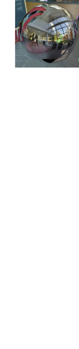
ptg11539634

Chapter 7

Toward the 3D World

In the previous chapters, we used examples based on 2D geometrical shapes

to explain how the WebGL system works and how it supports the behavior

of shaders, transformations such as translation and rotation, animation, and

texture mapping. However, the techniques you’ve learned so far can be applied

not only to 2D shapes but also to 3D objects. In this chapter you’ll take the first

step into the 3D world and explore the implications of moving from 2D to 3D.

In particular, you will explore:

• Representing the user’s view into the 3D world

• Controlling the volume of 3D space that is viewed

• Clipping

• Handling foreground and background objects

• Drawing a 3D object (a cube)

All these issues have a significant impact on how the 3D scene is drawn and

presented to viewers, and a mastery of them is critical to building compel-

ling 3D scenes. As usual, we’ll take you step by step so you will quickly master

the basics and be able to move on to the more complex issues of lighting and

performance in the final chapters.

What’s Good for Triangles Is Good for Cubes

So far, you’ve used the humble triangle in many of the explorations and

programs. As previously discussed, you’ve seen how 3D objects are composed

of 2D shapes—in particular the triangle. Figure 7.1 shows a cube that has been

built up from 12 triangles.

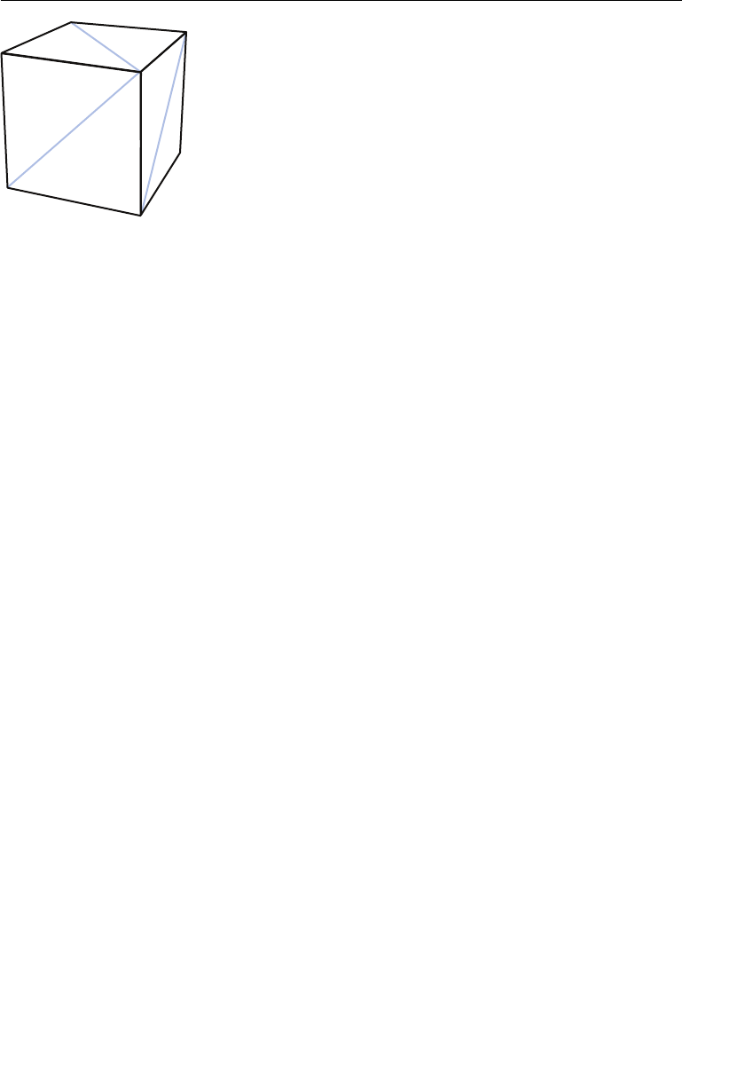
ptg11539634

CHAPTER 7 Toward the 3D World

226

Figure 7.1 A cube composed of triangles

So when you deal with 3D objects, you just need to apply the techniques you have

learned to each triangle that makes up the objects. The only difference from past exam-

ples, and it’s a significant one, is that you now need to consider the depth information

of the triangles in addition to the x and y coordinates. Let’s begin by exploring how you

specify and control the viewing direction—that is, the view into the 3D scene the user

has—and then look at the visible range that controls how much of the scene the user sees.

The explanations focus on the basic triangle because it simplifies things; however, what’s

true for triangles is true for 3D objects.

Specifying the Viewing Direction

The critical factor when considering 3D objects is that they have depth in a 3D space.

This means you need to take care of several issues that you didn’t have to consider when

using 2D shapes. First, because of the nature of 3D space, you can look at the object from

anywhere in the space; that is, your viewpoint can be anywhere. When describing the way

you view objects, two important points need consideration:

• The viewing direction (where you are looking from, and at which part of the scene

are you looking?)

• The visible range (given the viewing direction, where can you actually see?)

In this first section let’s explore viewing direction and the techniques that allow you to

place the eye point anywhere in 3D space and then look at objects from various direc-

tions. You’ll take a look at the second item and see how to specify the visible range in the

next section.

As introduced in Chapter 2 , “Your First Step with WebGL” (refer to Figure 2.16 ), let’s

assume that, by default, the eye point is placed at the origin (0, 0, 0), and the line of sight

extends along the z-axis in the negative direction (inward toward your computer screen).

In this section, you will move the eye point from the default location to other locations

and then view a triangle from there.

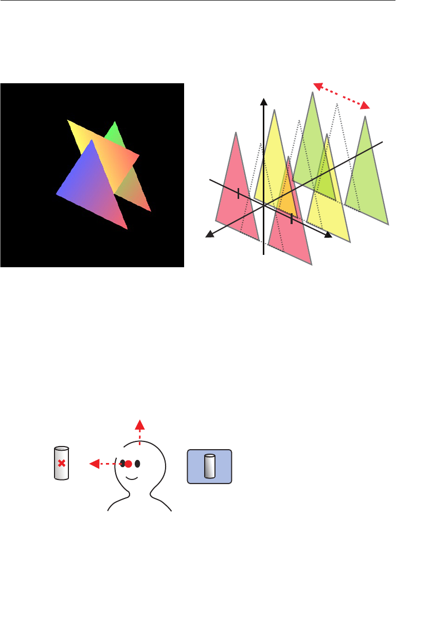
ptg11539634

Specifying the Viewing Direction 227

Let’s construct a sample program, LookAtTriangles , that locates the eye point at (0.20,

0.25, 0.25) and then views three triangles from there toward the origin (0, 0, 0). Using

three triangles makes it easy to understand the depth information in the 3D scene. Figure

7.2 shows a screen shot of

LookAtTriangles and the color and z coordinate of each

triangle.

Figure 7.2 LookAtTriangles (left), and the color and z coordinate of each triangle (right)

The program uses softer colors because they are easier on the eyes.

Eye Point, Look-At Point, and Up Direction

To specify where you are looking from and which part of the scene you are looking at in

the 3D space, you need two items of position information: the eye point (where you are

looking from) and the look-at point (which part of the scene you are looking at). In addi-

tion, in 3DCG, you need to specify which direction is up in the scene. As such, a total of

three items of information are required to specify the viewing direction (see Figure 7.3 ).

rotcevpu

tniopta—kool

enecs

)Zeye,Yeye,Xeye(

)Zpu,Ypu,Xpu(

)Zta,Yta,Xta(

tniopeye

Figure 7.3 Eye point, look-at point, and up direction

-0.75

0.75

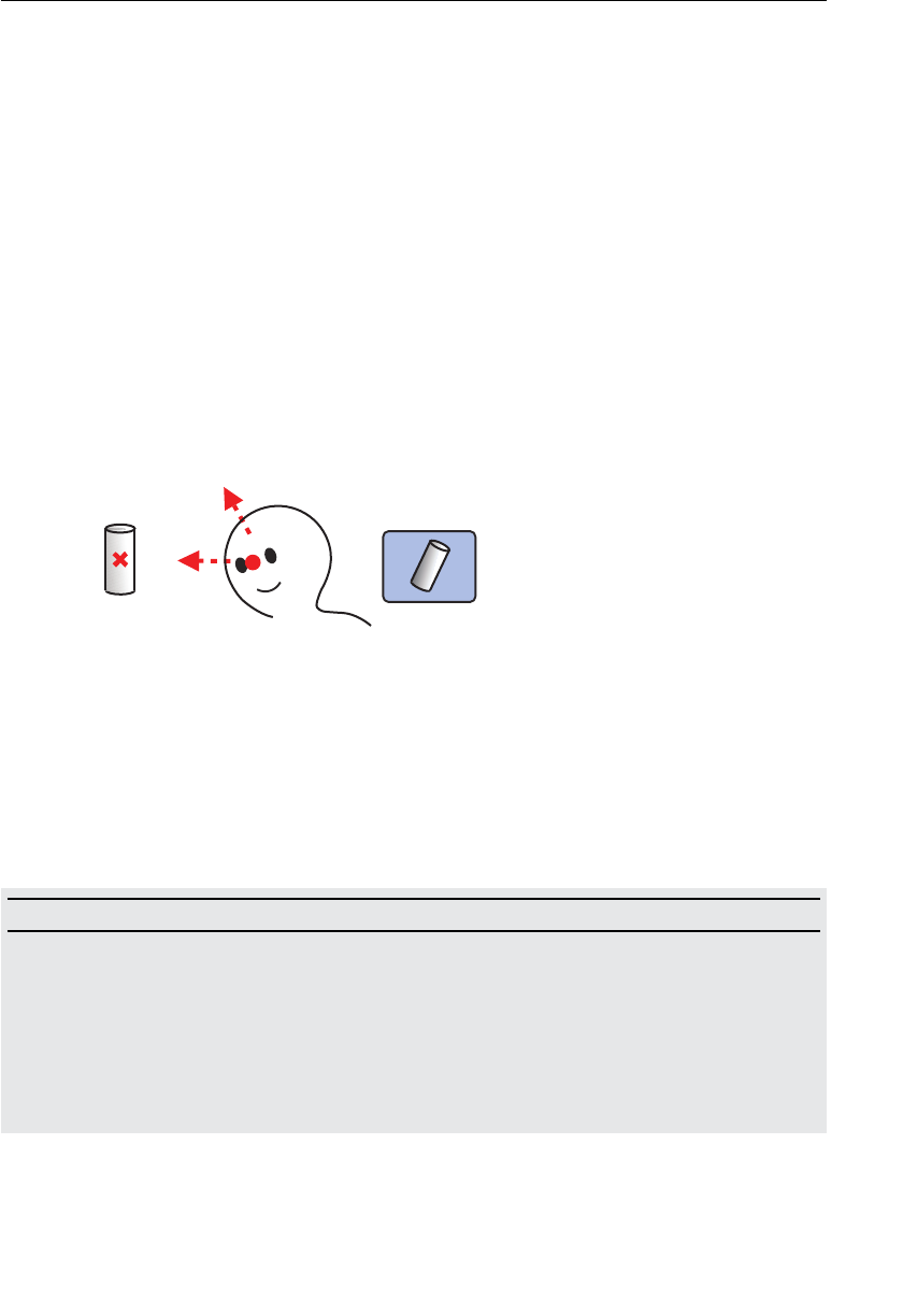
ptg11539634

CHAPTER 7 Toward the 3D World

228

Eye point: This is the starting point from which the 3D space is viewed. In the following

sections, the coordinates of this position are referred to as (eyeX, eyeY, eyeZ).

Look-at point: This is the point at which you are looking and which determines the

direction of the line of sight from the eye point. As the name suggests, the eye point is a

point, not a vector, so another point (such as the look-at point) is required to determine

the direction in which you are looking. The look-at point is a point on the line of sight

extending from the eye point. The coordinates of the look-at point are referred to as

(atX, atY, atZ).

Up direction: This determines the up direction in the scene that is being viewed from

the eye point to the look-at point. If only the eye point and the look-at point are deter-

mined, there is freedom to rotate the line of sight from the eye point to the look-at

point. (In Figure 7.4 , inclining the head causes the top and bottom of the scene to shift.)

To define the rotation, you must determine the up direction along the line of sight. The

up direction is specified by three numbers representing the direction. The coordinates for

this direction are referred to as (upX, upY, upZ).

rotcevpu

tniopta—kool

enecs

tniopeye

Figure 7.4 Eye point, look-at point, and up direction

In WebGL, you can specify the position and direction the eye point faces by converting

these three items of information in a matrix and passing the matrix to a vertex shader.

This matrix is called a view transformation matrix or view matrix , because it changes

the view of the scene. In

cuon-matrix.js , the method Matrix4.setLookAt() is defined

to calculate the view matrix from the three items of information: eye point, look-at point

and up direction.

Matrix4.setLookAt(eyeX, eyeY, eyeZ, atX, atY, atZ, upX, upY, upZ)

Calculate the view matrix derived from the eye point ( eyeX , eyeY , eyeZ ), the look-at point

( atX , atY , atZ ), and the up direction ( upX , upY , upZ ). This view matrix is set up in the

Matrix4 object. The look-at point is mapped to the center of the

<canvas> .

Parameters eyeX, eyeY, eyeZ Specify the position of the eye point .

atX, atY, atZ Specify the position of the look-at point .

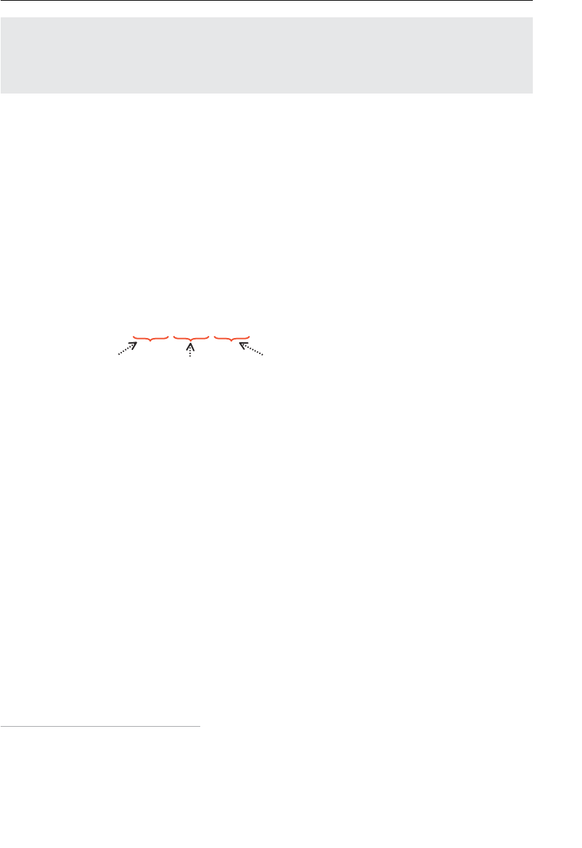
ptg11539634

Specifying the Viewing Direction 229

upX, upY, upZ Specify the up direction in the scene. If the up direction is

along the positive y-axis, then ( upX , upY , upZ ) is (0, 1, 0).

Return value None

In WebGL, the default settings when using

Matrix4.setLookAt() are defined as follows:

• The eye point is placed at (0, 0, 0) (that is, the origin of the coordinate system).

• The look-at point is along the negative z-axis, so a good value is (0, 0, –1) .1 The up

direction is specified along the positive y-axis, so a good value is (0, 1, 0).

So, for example, if the up direction is specified as (1, 0, 0), the positive x-axis becomes the

up direction; in this case, you will see the scene tilted by 90 degrees.

A view matrix representing the default settings in WebGL can be simply produced as

follows (see Figure 7.5 ).

;)(4xirtaMwen=xirtaMweiVlaitinirav

;)0,1,0,1—,0,0,0,0,0(tAkooLtes.xirtaMweiVlaitini

rotcevputniopta—kooltniopeye

Figure 7.5 An example of setLookAt()

Now you understand how to use the method

setLookAt() , so let’s take a look at its use in

an actual sample program.

Sample Program (LookAtTriangles.js)

LookAtTriangles.js , shown in Listing 7.1 , is a program that changes the position of the

eye point and then draws the three triangles shown in Figure 7.2 . Although it is difficult

to see on paper, the three triangles are, in order of proximity, blue, yellow, and green,

respectively, all fading to red in the bottom-right corner.

Listing 7.1 LookAtTriangles.js

1 // LookAtTriangles.js

2 // Vertex shader program

3 var VSHADER_SOURCE =

4 ‘attribute vec4 a_Position;n’ +

5 ‘attribute vec4 a_Color;n’ +

6 ‘uniform mat4 u_ViewMatrix;n’ +

1 The z component could be any negative value. The value -1 is an example but we could have chosen

any other negative value.

ptg11539634

CHAPTER 7 Toward the 3D World

230

7 ‘varying vec4 v_Color;n’ +

8 ‘void main() {n’ +

9 ‘ gl_Position = u_ViewMatrix * a_Position;n’ +

10 ‘ v_Color = a_Color;n’ +

11 ‘}n’;

13 // Fragment shader program

14 var FSHADER_SOURCE =

…

18 ‘varying vec4 v_Color;n’ +

19 ‘void main() {n’ +

20 ‘ gl_FragColor = v_Color;n’ +

21 ‘}n’;

23 function main() {

…

40 // Set the vertex coordinates and color (blue triangle is in front)

41 var n = initVertexBuffers(gl);

…

50 // Get the storage location of u_ViewMatrix variable

51 var u_ViewMatrix = gl.getUniformLocation(gl.program,’u_ViewMatrix’);

…

57 // Set the eye point, look-at point, and up direction

58 var viewMatrix = new Matrix4();

59 viewMatrix.setLookAt(0.20, 0.25, 0.25, 0, 0, 0, 0, 1, 0);

61 // Pass the view matrix to u_ViewMatrix variable

62 gl.uniformMatrix4fv(u_ViewMatrix, false, viewMatrix.elements);

…

67 // Draw a triangle

68 gl.drawArrays(gl.TRIANGLES, 0, n);

69 }

71 function initVertexBuffers(gl) {

72 var verticesColors = new Float32Array([

73 // vertex coordinates and color

74 0.0, 0.5, -0.4, 0.4 1.0, 0.4, // The back green triangle

75 -0.5, -0.5, -0.4, 0.4 1.0, 0.4,

76 0.5, -0.5, -0.4, 1.0, 0.4 0.4,

78 0.5, 0.4, -0.2, 1.0, 0.4 0.4, // The middle yellow triangle

79 -0.5, 0.4, -0.2, 1.0, 1.0, 0.4,

80 0.0, -0.6, -0.2, 1.0, 1.0, 0.4,

82 0.0, 0.5, 0.0, 0.4 0.4 1.0, // The front blue triangle

ptg11539634

Specifying the Viewing Direction 231

83 -0.5, -0.5, 0.0, 0.4 0.4 1.0,

84 0.5, -0.5, 0.0, 1.0, 0.4 0.4

85 ]);

86 var n = 9;

88 // Create a buffer object

89 var vertexColorbuffer = gl.createBuffer();

…

96 gl.bindBuffer(gl.ARRAY_BUFFER, vertexColorbuffer);

97 gl.bufferData(gl.ARRAY_BUFFER, verticesColors, gl.STATIC_DRAW);

…

121 return n;

122 }

This program is based on ColoredTriangle.js in Chapter 5 , “Using Colors and Texture

Images.” The fragment shader, the method of passing the vertex information, and so on,

is the same as in

ColoredTriangle.js . The three main differences follow:

• The view matrix is passed to the vertex shader (line 6) and then multiplied by the

vertex coordinates (line 9).

• The vertex coordinates and color values of the three triangles (line 72 to 85) are set

up in

initVertexBuffers() , which is called from line 41 of main() in JavaScript.

• The view matrix is calculated at lines 58 and 59 in main() and passed to the uniform

variable

u_ViewMatrix in the vertex shader at line 62. You should note that the posi-

tion of the eye point is (0.2, 0.25, 0.25); the position of the look-at point is (0, 0, 0);

the up direction is (0, 1, 0).

Let’s start by looking at the second difference and the function

initVertexBuffers() (line

71). The difference between this program and the original program,

ColoredTriangle.

js , is that verticesColors at line 72 (which is the array of vertex coordinates and colors

for a single triangle) is modified for the three triangles, and the z coordinates are added

in the array. These coordinates and colors are stored together in the buffer object

vertex-

ColorBuffer (lines 96 and 97) created at line 89. Because you are now dealing with three

triangles (each with three vertices), you need to specify 9 as the third argument of

gl.

drawArrays() at line 68.

To specify the view matrix (that is, where you are looking and which part of the scene you

are looking at [item 3]), you need to set up and pass the view matrix to the vertex shader.

To do this, a

Matrix4 object viewMatrix is created at line 58, and you use setLookAt() to

calculate and store the view matrix to

viewMatrix at line 59. This view matrix is passed to

u_ViewMatrix at line 62, which is the uniform variable used in the vertex shader:

57 // Set the eye point, look-at point, and up direction

58 var viewMatrix = new Matrix4();

59 viewMatrix.setLookAt(0.20, 0.25, 0.25, 0, 0, 0, 0, 1, 0);

ptg11539634

CHAPTER 7 Toward the 3D World

232

61 // Pass the view matrix to the u_ViewMatrix variable

62 gl.uniformMatrix4fv(u_ViewMatrix, false, viewMatrix.elements);

Those are all the changes needed in the JavaScript program. Now let’s examine what is

happening in the vertex shader:

2 // Vertex shader program

3 var VSHADER_SOURCE =

4 ‘attribute vec4 a_Position;n’ +

5 ‘attribute vec4 a_Color;n’ +

6 ‘uniform mat4 u_ViewMatrix;n’ +

7 ‘varying vec4 v_Color;n’ +

8 ‘void main() {n’ +

9 ‘ gl_Position = u_ViewMatrix * a_Position;n’ +

10 ‘ v_Color = a_Color;n’ +

11 ‘}n’;

The vertex shader starts from line 4. The only two lines that differ from ColoredTriangle.

js are indicated by boldface: Line 6 defines the uniform variable u_ViewMatrix , and line 9

multiplies the matrix by the vertex coordinates. These modifications seem quite trivial, so

how do they change the position of the eye point?

Comparing LookAtTriangles.js with RotatedTriangle_Matrix4.js

Looking at the vertex shader in this sample program, you may notice a similarity

with that in

RotatedTriangle_Matrix4.js , which was explained in Chapter 4 , “More

Transformations and Basic Animation.” That vertex shader created a rotation matrix using

Matrix4 object and then used the matrix to rotate a triangle. Let’s take a look at that

shader again:

1 // RotatedTriangle_Matrix4.js

2 // Vertex shader program

3 var VSHADER_SOURCE =

4 ‘attribute vec4 a_Position;n’ +

5 ‘uniform mat4 u_rotMatrix;n’ +

6 ‘void main() {n’ +

7 ‘ gl_Position = u_rotMatrix * a_Position;n’ +

8 ‘}n’;

The vertex shader in this section ( LookAtTriangles.js ) is listed as follows:

1 // LookAtTriangles.js

2 // Vertex shader program

3 var VSHADER_SOURCE =

4 ‘attribute vec4 a_Position;n’ +

5 ‘attribute vec4 a_Color;n’ +

6 ‘uniform mat4 u_ViewMatrix;n’ +

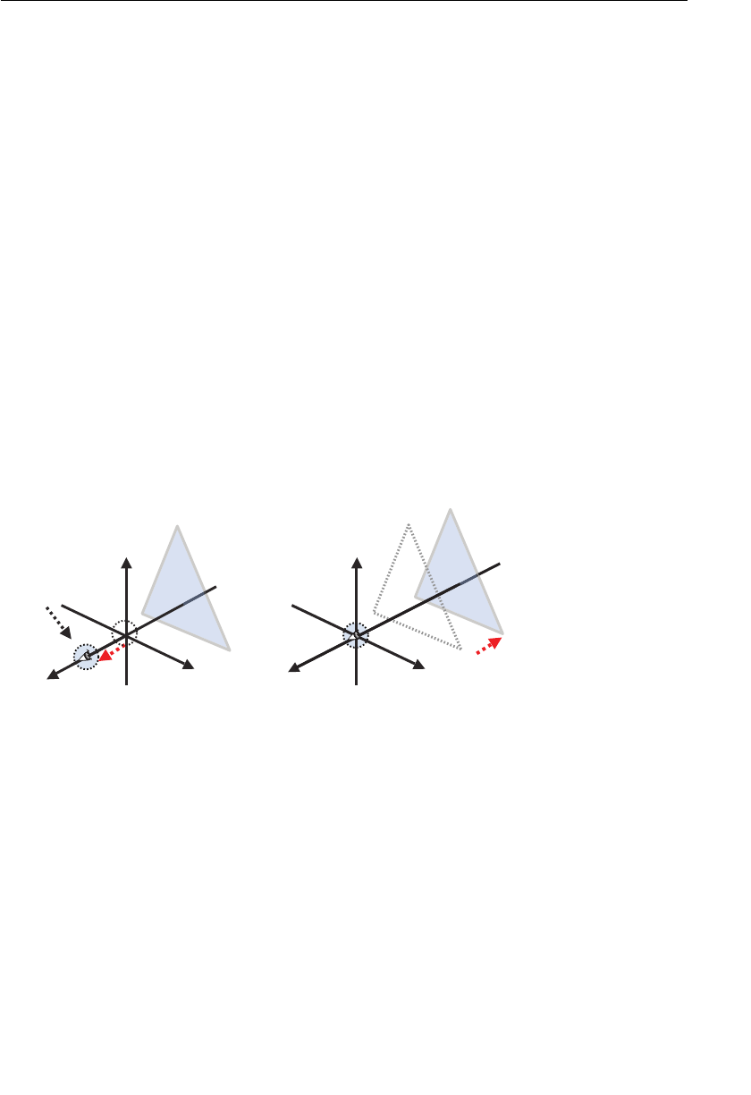
ptg11539634

Specifying the Viewing Direction 233

7 ‘varying vec4 v_Color;n’ +

8 ‘void main() {n’ +

9 ‘ gl_Position = u_ViewMatrix * a_Position;n’ +

10 ‘ v_Color = a_Color;n’ +

11 ‘}n’;

As you can see, the attribute variable for color values ( a_Color ) and the varying variable

that passes the values to the fragment shader (

v_Color ) were added, and the name of the

uniform variable was changed from

u_rotMatrix to u_ViewMatrix . Despite these differ-

ences, the calculation of the value assigned to

gl_Position is the same as that in the

vertex shader of

RotatedTriangle_Matrix4.js : multiplying a mat4 matrix by a_Position .

(Compare line 7 in

RotatedTriangle_Matrix4.js with line 9 in LookAtTriangles.js .)

This tells you that the operation performing “where you are looking and which part of the

scene you are looking at” is actually equivalent to transformations such as translating or

rotating a triangle.

Let’s use an example to explain this. Assume that you are looking at a triangle from the

origin (0, 0, 0) along the negative direction of the z-axis, and then the eye point moves to

the position (0, 0, 1) (the left-side figure of Figure 7.6 ). In this case, the distance between

the eye point and the triangle has increased by 1.0 unit of the z-axis. To achieve the same

effect, you could leave the eye point alone and instead move the triangle 1.0 unit away

(the right-side figure of Figure 7.6 ).

tniopeye

Figure 7.6 Movement of the eye point is identical to that of objects in the scene

This is exactly what happens in our sample program. The

setLookAt() method of the

Matrix4 object just calculates the matrix to carry out this transformation using the infor-

mation about the position of the eye point, look-at point, and up direction. So, by then

multiplying the matrix by the vertex coordinates of the objects in the scene, you obtain

the same effect as moving the eye point. Essentially, instead of moving the eye point

in one direction, the objects viewed (that is, the world itself) are moved in the opposite

direction. You can use the same approach to handle rotation of the eye point.

Because moving the eye point is the same type of transformation as rotating or translating

a triangle, you can represent both of them as a transformation matrix. Let’s look at how

ptg11539634

CHAPTER 7 Toward the 3D World

234

you calculate the matrix when you want to rotate a triangle and move the position of the

eye point.

Looking at Rotated Triangles from a Specified Position

RotatedTriangle_Matrix4 in Chapter 4 displayed the triangle rotated around the z-axis. In

this section, you modify

LookAtTriangles to display the triangles viewed from a specified

eye point along the line of sight. In this case, two matrices are required: a rotation matrix

to rotate the triangles and a view matrix to specify the view of the scene. The first issue to

consider is in which order you should multiply them.

So far, you know that multiplying a matrix by a vertex coordinate will apply the trans-

formation defined by the matrix to the coordinates. That is to say, multiplying a rotation

matrix by a vertex coordinate causes it to be rotated.

Multiplying a view matrix by a vertex coordinate causes the vertex to be transformed to

the correct position as viewed from the eye position. In this sample program, we want to

view the rotated triangles from a specified position, so we need to rotate the triangles and

then look at them from the specified eye position. In other words, we need to rotate the

three vertex coordinates comprising the triangle. Then we need to transform the rotated

vertex coordinates (the rotated triangle) as we look at them from the specified position.

We can achieve this by carrying out a matrix multiplication in the order described in the

previous sentence. Let’s check the equations.

As explained previously, if you want to rotate a shape, you need to multiply a rotation

matrix by the vertex coordinates of the shape as follows:

〈〉=

〈〉×〈〉

rotated vertex coordinates

rotation matrix original vertex coordinates

«» 



By multiplying a view matrix by the rotated vertex coordinates in the preceding equation,

you can obtain the rotated vertex coordinates that are viewed from the specified position.

〈〉=

〈〉×〈〉

rotated vertex coordinates viewed from specified position

view matrix rotated vertex coordinates

«» «  «

«»

If you substitute the first expression into the second one, you obtain the following:

〈〉=

〈〉×〈〉×〈〉

rotated vertex coordinates viewed from specified position

view matrix rotation matrix original vertex coordinates

«» «  «



In this expression, you use a rotation matrix, but you can also apply a translation matrix,

a scaling matrix, or a combination of them. Such a matrix is generally called a model

matrix . Using that term, you can rewrite the expression shown in Equation 7.1 .

Equation 7.1

〈〉×〈〉×〈〉view matrix model matrix vertex coordinates

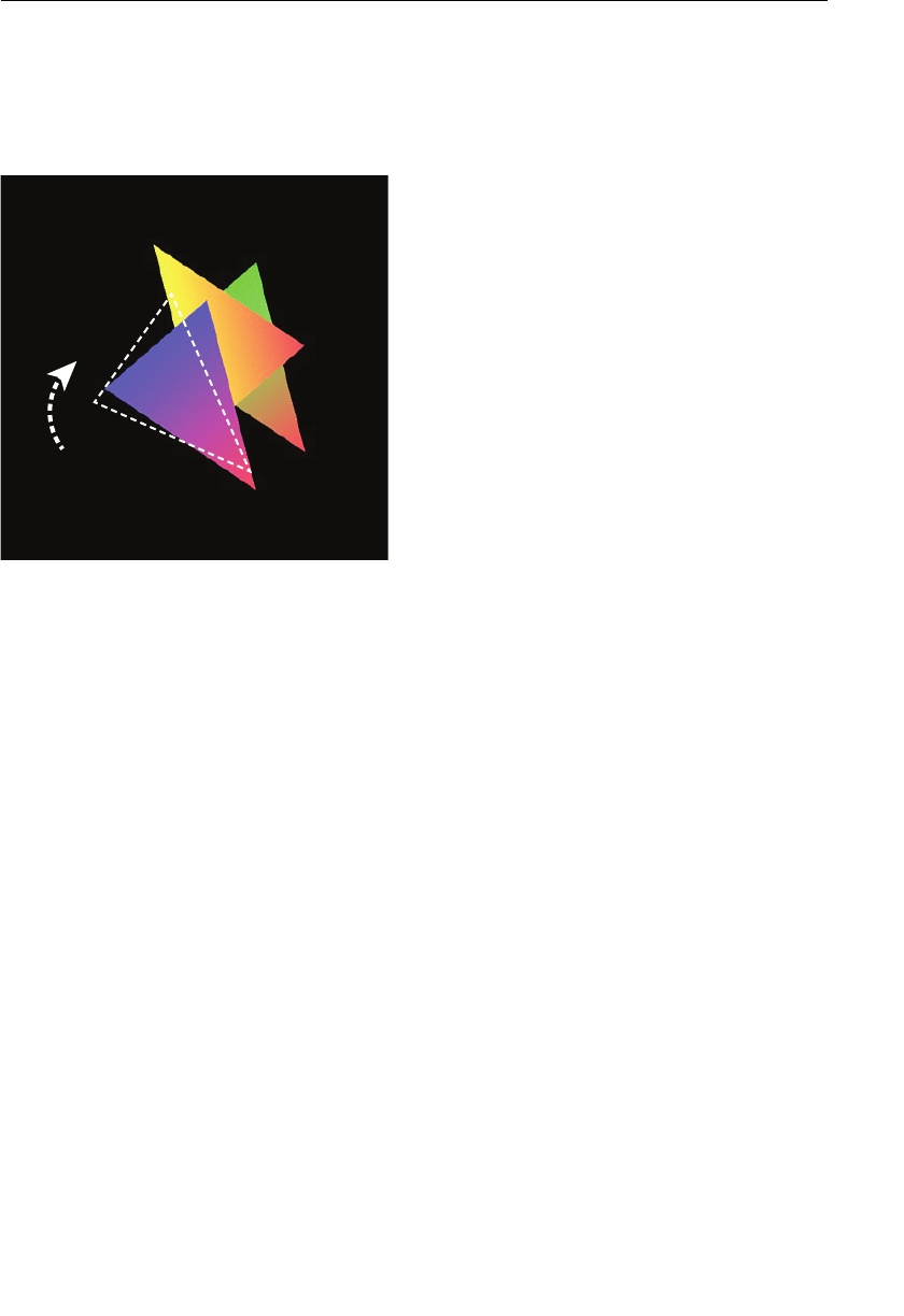
ptg11539634

Specifying the Viewing Direction 235

Now you need to implement this expression in a shader program, but because it is quite

a simple expression, you can implement it as-is in a vertex shader. The sample program

LookAtRotatedTriangles implements the transformation, and a screen shot is shown in

Figure 7.7 . Note, in this figure, that the white dashed line shows the triangle before rota-

tion so that you can easily see the rotation.

Figure 7.7 LookAtRotatedTriangles

Sample Program (LookAtRotatedTriangles.js)

LookAtRotatedTriangles.js is programmed by slightly modifying LookAtTriangles.js .

You just need to add the uniform variable

u_ModelMatrix to pass the model matrix to the

shader and then add some processing in JavaScript’s

main() function to pass the matrix to

the variable. The relevant code is shown in Listing 7.2 .

Listing 7.2 LookAtRotatedTriangles.js

1 // LookAtRotatedTriangles.js

2 // Vertex shader program

3 var VSHADER_SOURCE =

4 ‘attribute vec4 a_Position;n’ +

5 ‘attribute vec4 a_Color;n’ +

6 ‘uniform mat4 u_ViewMatrix;n’ +

7 ‘uniform mat4 u_ModelMatrix;n’ +

8 ‘varying vec4 v_Color;n’ +

9 ‘void main() {n’ +

10 ‘ gl_Position = u_ViewMatrix * u_ModelMatrix * a_Position;n’ +

11 ‘ v_Color = a_Color;n’ +

12 ‘}n’;

…

ptg11539634

CHAPTER 7 Toward the 3D World

236

24 function main() {

…

51 // Get the storage locations of u_ViewMatrix and u_ModelMatrix

52 varu_ViewMatrix = gl.getUniformLocation(gl.program,’u_ViewMatrix’);

53 var u_ModelMatrix = gl.getUniformLocation(gl.program, ‘u_ModelMatrix’);

…

59 // Specify the eye point and line of sight

60 var viewMatrix = new Matrix4();

61 viewMatrix.setLookAt(0.20, 0.25, 0.25, 0, 0, 0, 0, 1, 0);

63 // Calculate the rotation matrix

64 var modelMatrix = new Matrix4();

65 modelMatrix.setRotate(-10, 0, 0, 1); // Rotate around z-axis

67 // Pass each matrix to each uniform variable

68 gl.uniformMatrix4fv(u_ViewMatrix, false, viewMatrix.elements);

69 gl.uniformMatrix4fv(u_ModelMatrix, false, modelMatrix.elements);

First, let’s examine the vertex shader. You can see that line 10 simply implements

Equation 7.1 as-is by using

u_ModelMatrix at line 7, which receives data from the

JavaScript program:

10 ‘ gl_Position = u_ViewMatrix * u_ModelMatrix * a_Position;n’ +

In the main() function in JavaScript, you already have the code for calculating a view

matrix, so you just need to add the code for calculating the rotation matrix perform-

ing a –10 degree rotation around the z-axis. Line 53 gets the storage location of the

u_ModelMatrix variable, and line 64 creates modelMatrix for the rotation matrix. Then

line 65 calculates the matrix using

Matrix4.setRotate() , and line 69 passes it to

u_ModelMatrix .

When you run this sample program, you will see the triangles shown in Figure 7.6 illus-

trating that the matrices multiplied by the vertex coordinates (

a_Position ) have the

desired effect. That is, the vertex coordinates were rotated by

u_ModelMatrix , and then

the resulting coordinates were transformed by

u_ViewMatrix to the correct position as if

viewed from the specified position.

Experimenting with the Sample Program

In LookAtRotatedTriangles.js , you implemented Equation 7.1 as- is. However, because

the multiplication of the view matrix and model matrix is performed per vertex in the

vertex shader, this implementation is inefficient when processing many vertices. The

result of the matrix multiplication in Equation 7.1 is identical for each vertex, so you can

calculate it in advance and pass the result to the vertex shader. The matrix obtained by

multiplying a view matrix by a model matrix is called a model view matrix . That is,

ptg11539634

Specifying the Viewing Direction 237

〈〉=〈〉×〈〉model view matrix view matrix model matrix   

Then, you can rewrite the expression in Equation 7.1 as shown in Equation 7.2 .

Equation 7.2

〈〉×〈〉model view matrix vertex coordinates 

If you use Equation 7.2 , you can rewrite the sample program shown in Listing 7.3 . This

sample program is LookAtRotatedTriangles_mvMatrix .

Listing 7.3 LookAtRotatedTriangles_mvMatrix.js

1 // LookAtRotatedTriangles_mvMatrix.js

2 // Vertex shader program

3 var VSHADER_SOURCE =

…

6 ‘uniform mat4 u_ModelViewMatrix;n’ +

7 ‘varying vec4 v_Color;n’ +

8 ‘void main() {n’ +

9 ‘ gl_Position = u_ModelViewMatrix * a_Position;n’ +

10 ‘ v_Color = a_Color;n’ +

11 ‘}n’;

…

23 function main() {

…

50 // Get the storage locations of u_ModelViewMatrix and u_ModelMatrix

51 var u_ModelViewMatrix = gl.getUniformLocation(gl.program, ‘u_ModelViewMatrix’);

…

59 viewMatrix.setLookAt(0.20, 0.25, 0.25, 0, 0, 0, 0, 1, 0);

…

63 modelMatrix.setRotate(-10, 0, 0, 1); // Calculate rotation matrix

65 // Multiply both matrices

66 var modelViewMatrix = viewMatrix.multiply(modelMatrix);

68 // Pass the model viewmatrix to u_ModelViewMatrix

69 gl.uniformMatrix4fv(u_ModelViewMatrix, false, modelViewMatrix.elements);

In the vertex shader, the name of the uniform variable was modified to u_

ModelViewMatrix and calculated in line 9. However, the processing steps in the vertex

shader are identical to the original

LookAtTriangles.js .

Within the JavaScript program, the method of calculating viewMatrix and modelMatrix

from lines 59 to 63 is identical to that in

LookAtRotatedTriangles.js and, when multi-

plied, result in

modelViewMatrix (line 66). The multiply() method is used to multiply

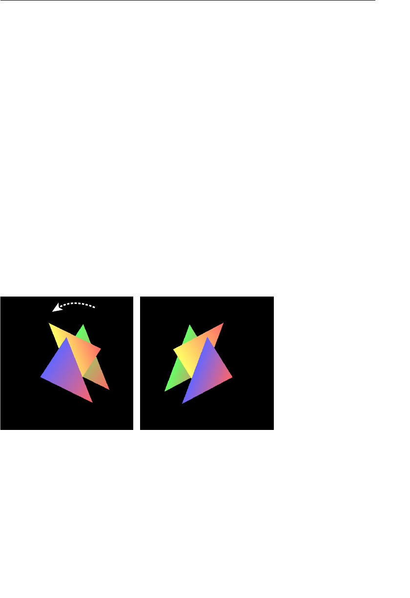
ptg11539634

CHAPTER 7 Toward the 3D World

238

Matrix4 objects. It multiplies the matrix on the right side ( viewMatrix ) by the matrix

specified by the argument (

modelMatrix ) of the method. So this code actually performs

modelViewMatrix= viewMatrix * modelMatrix . Unlike with GLSL ES, you need to use a

method to perform matrix multiplication instead of the

* operator.

Having obtained modelViewMatrix , you just need to pass it to the u_ModelViewMatrix

variable at line 69. Once you run the program, you can see the same result as shown in

Figure 7.6 .

As a final point, in this sample program, each matrix was calculated piece by piece at lines

59, 63, and 66 to better show the flow of the calculation. However, this could be rewritten

in one line for efficiency:

var modelViewMatrix = new Matrix4();

modelViewMatrix.setLookAt(0.20, 0.25, 0.25, 0, 0, 0, 0, 1, 0).rotate(-10, 0, 0, 1);

// Pass the model view matrix to the uniform variable

gl.uniformMatrix4fv(u_ModelViewMatrix, false, modelViewMatrix.elements);

Changing the Eye Point Using the Keyboard

Let’s modify LookAtTriangles to change the position of the eye point when the arrow

keys are pressed.

LookAtTrianglesWithKeys uses the right arrow key to increase the x coor-

dinate of the eye point by 0.01 and the left arrow key to decrease the coordinate by 0.01.

Figure 7.8 shows a screen shot of the sample program when run. If you hold down the left

arrow key, the scene changes to that seen on the right side of Figure 7.8 .

Figure 7.8 LookAtTrianglesWithKeys

Sample Program (LookAtTrianglesWithKeys.js)

Listing 7.4 shows the sample code. The vertex shader and the fragment shader are the

same as those in

LookAtTriangles.js . The basic processing flow of main() in JavaScript

is also the same. The code for registering the event handler called on a key press is added

ptg11539634

Specifying the Viewing Direction 239

to the sample program, and the code for drawing the triangles has been moved into the

function

draw() .

Listing 7.4 LookAtTrianglesWithKeys.js

1 // LookAtTrianglesWithKeys.js

2 // Vertex shader program

3 var VSHADER_SOURCE =

4 ‘attribute vec4 a_Position;n’ +

5 ‘attribute vec4 a_Color;n’ +

6 ‘uniform mat4 u_ViewMatrix;n’ +

7 ‘varying vec4 v_Color;n’ +

8 ‘void main() {n’ +

9 ‘ gl_Position = u_ViewMatrix * a_Position;n’ +

10 ‘ v_Color = a_Color;n’ +

11 ‘}n’;

…

23 function main() {

…

50 // Get the storage location of the u_ViewMatrix variable

51 varu_ViewMatrix = gl.getUniformLocation(gl.program,’u_ViewMatrix’);

…

57 // Create Matrix4 object for a view matrix

58 var viewMatrix = new Matrix4();

59 // Register the event handler to be called on key press

60 document.onkeydown = function(ev){ keydown(ev, gl, n, u_ViewMatrix,

➥viewMatrix); };

62 draw(gl, n, u_ViewMatrix, viewMatrix); // Draw a triangle

63 }

…

117 var g_eyeX = 0.20, g_eyeY = 0.25, g_eyeZ = 0.25; // The eye point

118 function keydown(ev, gl, n, u_ViewMatrix, viewMatrix) {

119 if(ev.keyCode == 39) { // The right arrow key was pressed

120 g_eyeX += 0.01;

121 } else

122 if (ev.keyCode == 37) { // The left arrow key was pressed

123 g_eyeX -= 0.01;

124 } else { return; } // Prevent unnecessary drawing

125 draw(gl, n, u_ViewMatrix, viewMatrix);

126 }

127

128 function draw(gl, n, u_ViewMatrix, viewMatrix) {

129 // Set the eye point and line of sight

130 viewMatrix.setLookAt(g_eyeX, g_eyeY, g_eyeZ, 0, 0, 0, 0, 1, 0);

ptg11539634

CHAPTER 7 Toward the 3D World

240

131

132 // Pass the view matrix to the u_ViewMatrix variable

133 gl.uniformMatrix4fv(u_ViewMatrix, false, viewMatrix.elements);

134

135 gl.clear(gl.COLOR_BUFFER_BIT); // Clear <canvas>

136

137 gl.drawArrays(gl.TRIANGLES, 0, n); // Draw a triangle

138 }

In this sample, you are using the event handler to change the position of the eye point

when the right arrow key or the left arrow key is pressed. Before explaining the event

handler, let’s look at the function

draw() that is called from the event handler.

The process performed in

draw() is straightforward. Line 130 calculates the view matrix

using the global variables

g_eyeX , g_eyeY , and g_eyeZ defined at line 117, which contain

0.2, 0.25, and 0.25, respectively. Then the matrix is passed to the uniform variable

u_ViewMatrix in the vertex shader at line 133. Back in main() , the storage location of

u_ViewMatrix is retrieved at line 51, and a Matrix4 object ( viewMatrix ) is created at line

58. These two operations are carried out in advance because it is redundant if you perform

them for each draw operation, particularly retrieving the storage. After that, line 135 clears

<canvas> , and line 137 draws the triangles.

The variables g_eyeX , g_eyeY , and g_eyeZ specify the eye position and are recalculated

in the event handler whenever a key is pressed. To call the event handler on key press,

you need to register it to the

onkeydown property of the document object. In this event

handler, because you need to call

draw() to draw the triangles, you must pass all argu-

ments that

draw() requires. This is why an anonymous function registers the handler as

follows:

59 // Register the event handler to be called on key press

60 document.onkeydown = function(ev){ keydown(ev, gl, n, u_ViewMatrix,

➥viewMatrix); };

This sets up the event handler keydown() to be called when the key is pressed. Let’s

examine how

keydown() is implemented.

118 function keydown(ev, gl, n, u_ViewMatrix, viewMatrix) {

119 if(ev.keyCode == 39) { // The right arrow key was pressed

120 g_eyeX += 0.01;

121 } else

122 if (ev.keyCode == 37) { // The left arrow key was pressed

123 g_eyeX -= 0.01;

124 } else { return ; } // Prevent unnecessary drawing

125 draw(gl, n, u_ViewMatrix, viewMatrix); // Draw a triangle

126 }

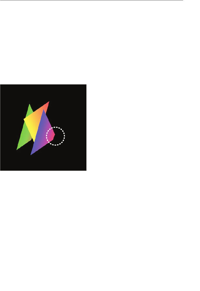
ptg11539634

Specifying the Visible Range (Box Type) 241

What keydown() is doing is also straightforward. When a key is pressed, keydown()

is called with the information about the event stored in the first parameter,

ev , of

keydown() . Then you just need to check which key was pressed by examining the value of

ev.keyCode , modify g_eyeX , and draw the triangles. When the right arrow key is pressed,

the code increases

g_eyeX by 0.01, and when the left arrow key is pressed, it decreases

g_eyeX by 0.01.

If you run the sample program, you can see the triangles shift every time you press the

arrow key.

Missing Parts

As you play with the sample program, you may notice that as you shift the eye position to

the extreme right or left, part of the triangle disappears (see Figure 7.9 ).

Figure 7.9 Part of the triangle disappears

This is because you haven’t specified the visible range (the boundaries of what you can

actually see) correctly. As mentioned in the first section of this chapter, WebGL does not

display objects outside the visible range. In the case of Figure 7.9 , part of the triangle went

out of the visible range while pressing the arrow keys.

Specifying the Visible Range (Box Type)

Although WebGL allows you to place 3D objects anywhere in 3D space, it only displays

those that are in the visible range. In WebGL, this is primarily a performance issue; there’s

no point in drawing 3D objects if they are not visible to the viewer. In a way, this mimics

the way human sight works (see Figure 7.10 ); we see objects within the visible range based

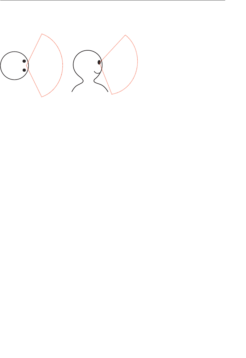
ptg11539634

CHAPTER 7 Toward the 3D World

242

on our line of sight, which is approximately 200 degrees in the horizontal field of view.

WebGL also has a similar limited range and does not display 3D objects outside of that

range.

Figure 7.10 Human visual field

In addition to the up/down, left/right range along the line of sight, WebGL has a depth

range that indicates how far you can see. These ranges are called the viewing volume . In

Figure 7.9 , because the depth range was not sufficient, part of the triangle disappears as it

moves out of the viewing volume.

Specify the Viewing Volume

There are two ways of specifying a viewing volume:

• Using a rectangular parallelepiped, or more informally, a box ( orthographic projec-

tion )

• Using a quadrangular pyramid ( perspective projection )

Perspective projection gives more information about depth and is often easier to view

because you use perspective views in real life. You should use this projection to show

the 3D scene in perspective, such as a character or a battlefield in a 3D shooting game.

Orthographic projection makes it much easier to compare two objects, such as two parts

of a molecule model, because there is no question about how the viewpoint may affect

the perception of distance. You should use the projection to show 3D objects in an ortho-

graphic view like those in technical drawing.

First, we will explain how the viewing volume works based on the box-shaped viewing

volume.

The box-shaped viewing volume is shaped as shown in Figure 7.11 . This viewing volume

is set from the eye point toward the line of sight and occupies the space delimited by the

two planes: the near clipping plane and the far clipping plane . The near clipping plane

is defined by ( right , top , — near ), (- left , top , — near ), (- left , — bottom , — near ), and ( right , — bottom ,

— near ). The far clipping plane is defined by ( right , top , — far ), (- left , top , — far ), (- left , — bottom ,

— far ), and ( right , — bottom , — far ).

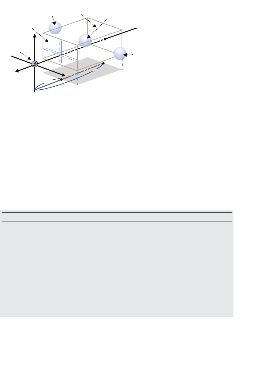
ptg11539634

Specifying the Visible Range (Box Type) 243

raen

raf

invisible visible

eye point left

right

bottom

top

far clipping plane

near clipping plane

invisible

Figure 7.11 Box-shaped viewing volume

The scene viewed from the near clipping plane toward the line of sight is displayed on the

<canvas> . If the aspect ratio of the near clipping plane is different from that of <canvas> ,

the scene is scaled according to the ratio, and the aspect ratio of the geometric shapes or

objects in the scene are distorted. (You will explore this behavior in the last part of this

section.) The range from the near clipping plane to the far clipping plane defines the

viewing volume. Only objects inside this volume are displayed. If the objects lie partially

inside the volume, only the part inside the volume is displayed.

Defining a Box—Shaped Viewing Volume

To set the box-shaped viewing volume, you use the method setOrtho() supported by the

Matrix4 object defined in cuon-matrix.js .

Matrix4.setOrtho(left, right, bottom, top, near, far)

Calculate the matrix (orthographic projection matrix) that defines the viewing volume

specified by its arguments, and store it in

Matrix4 . However, left must not be equal to

right , bottom not equal to top , and near not equal to far .

Parameters left, right Specify the distances to the left side and right side of the near

clipping plane.

bottom, top Specify the distances to the bottom and top of the near clipping

plane.

near, far Specify the distances to the near and far clipping planes along

the line of sight.

Return value None

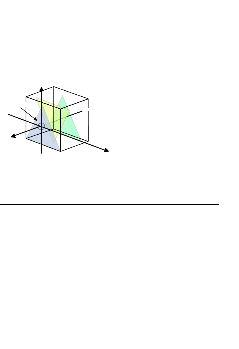
ptg11539634

CHAPTER 7 Toward the 3D World

244

Here, you are using a matrix again, which in this case is referred to as the ortho-

graphic projection matrix . The sample program

OrthoView will use this type of

projection matrix to set the box-shaped viewing volume and then draw three trian-

gles—as used in

LookAtRotatedTriangles —to test the effect of the viewing volume. In

LookAtRotatedTriangles , you placed the eye point at a different location from that of the

origin. However, in this sample program, you’ll use the origin (0, 0, 0) and set the line of

sight along the negative z-axis to make it easy to check the effect of the viewing volume.

The viewing volume is specified as shown in Figure 7.12 , which uses near =0.0, far =0.5,

left =–1.0, right =1.0, bottom =–1.0, and top =1.0 because the triangles lie between 0.0 and –0.4

along the z-axis (refer to Figure 7.2 ).

)0.0,0.1,0.1—(

)5.0—,0.1,0.1—(

)0.0,0.1—,0.1(

)0.0,0.1—,0.1—( )5.-0,0.1—,0.1—(

..)00,01,0.1(

. )-0.5,01,0.1(

tniopeye

Figure 7.12 The box-shaped viewing volume used in OrthoView

In addition, we add key-press event handlers to change the values of near and far to check

the effect of changing the size of the viewing volume. The following are the active keys

and their mappings.

Arrow Key Action

Right Increases near by 0.01

Left Decreases near by 0.01

Up Increases far by 0.01

Down Decreases far by 0.01

So that you can see the current values of near and far, they are displayed below the

canvas, as shown in Figure 7.13 .

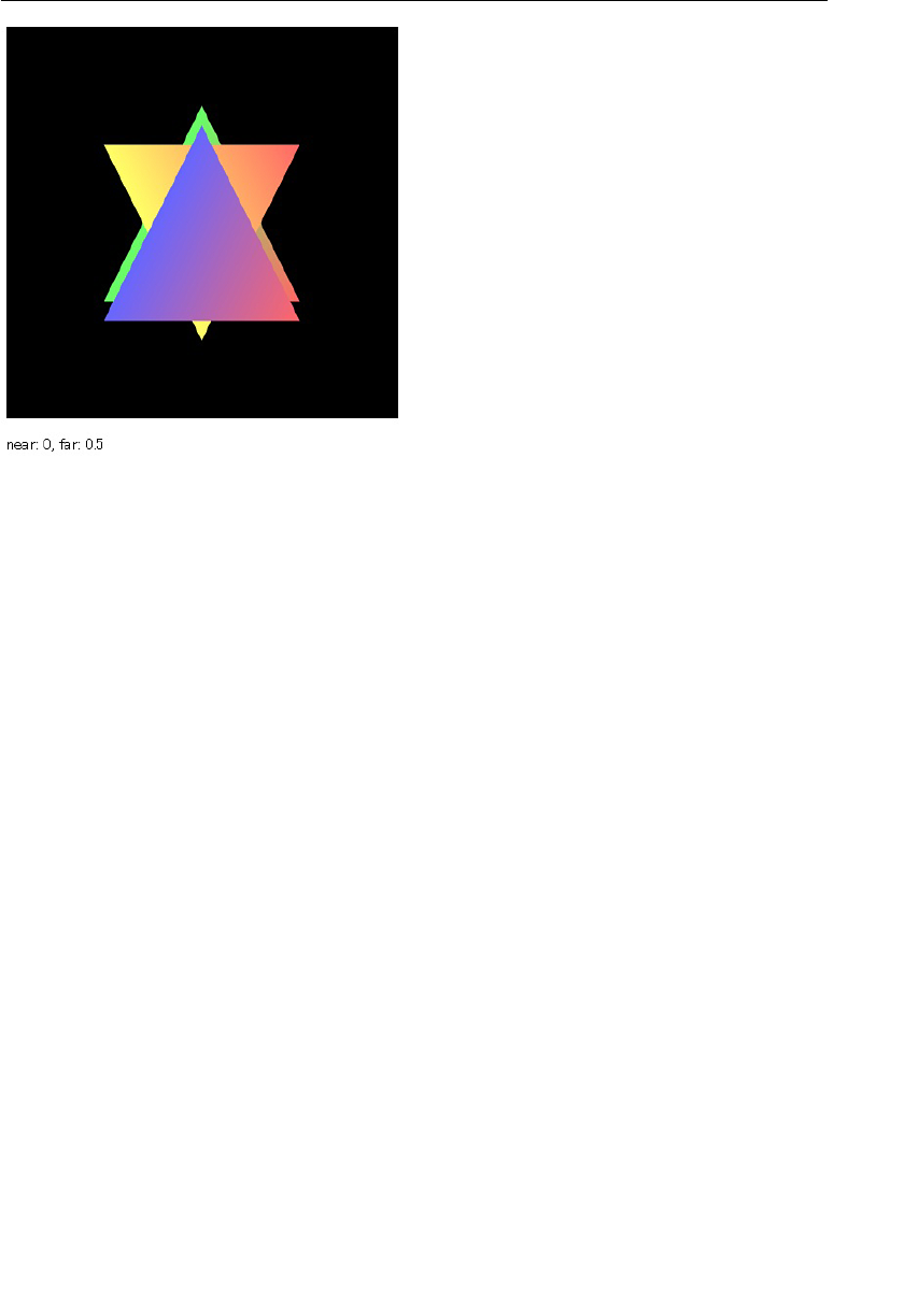
ptg11539634

Specifying the Visible Range (Box Type) 245

Figure 7.13 OrthoView

Let’s examine the sample program.

Sample Program (OrthoView.html)

Because this sample program shows the near and far value on the web page and not in

the

<canvas> , you need to add something to the HTML file listing as shown in Listing 7.5

(

OrthoView.html) .

Listing 7.5 OrthoView.html

1 <!DOCTYPE html>

2 <html>

3 <head lang=»ja»>

4 <meta charset=»utf-8″ />

5 <title>Set Box-shaped Viewing Volume</title>

6 </head>

8 <body onload=»main()»>

9 <canvas id=»webgl» width=»400″ height=»400″>

10 Please use a browser that supports <canvas>

11 </canvas>

12 <p id=»nearFar»> The near and far values are displayed here. </p>

14 <script src=»../lib/webgl-utils.js»></script>

…

18 <script src=»OrthoView.js»></script>

ptg11539634

CHAPTER 7 Toward the 3D World

246

19 </body>

20 </html>

As you can see, line 12 was added. This line shows “The near and far values are displayed

here” and uses JavaScript to rewrite the contents of

nearFar to show the current near and

far values.

Sample Program (OrthoView.js)

Listing 7.6 shows OrthoView.js . This program is almost the same as

LookAtTrianglesWithKeys.js , which changes the position of the eye point by using the

arrow keys.

Listing 7.6 OrthoView.js

1 // OrthoView.js

2 // Vertex shader program

3 var VSHADER_SOURCE =

4 ‘attribute vec4 a_Position;n’ +

5 ‘attribute vec4 a_Color;n’ +

6 ‘uniform mat4 u_ProjMatrix;n’ +

7 ‘varying vec4 v_Color;n’ +

8 ‘void main() {n’ +

9 ‘ gl_Position = u_ProjMatrix * a_Position;n’ +

10 ‘ v_Color = a_Color;n’ +

11 ‘}n’;

…

23 function main() {

24 // Retrieve<canvas> element

25 var canvas = document.getElementById(‘webgl’);

26 // Retrieve the nearFar element

27 var nf = document.getElementById(‘nearFar’);

…

52 // Get the storage location of u_ProjMatrix variable

53 var u_ProjMatrix = gl.getUniformLocation(gl.program,’u_ProjMatrix’);

…

59 // Create the matrix to set the eye point and line of sight

60 var projMatrix = new Matrix4();

61 // Register the event handler to be called on key press

62 document.onkeydown = function(ev) { keydown(ev, gl, n, u_ProjMatrix,

➥projMatrix, nf); };

64 draw(gl, n, u_ProjMatrix, projMatrix, nf); // Draw triangles

65 }

…

116 // The distances to the near and far clipping plane

ptg11539634

Specifying the Visible Range (Box Type) 247

117 var g_near = 0.0, g_far = 0.5;

118 function keydown(ev, gl, n, u_ProjMatrix, projMatrix, nf) {

119 switch(ev.keyCode) {

120 case 39: g_near += 0.01; break; // The right arrow key was pressed

121 case 37: g_near -= 0.01; break; // The left arrow key was pressed

122 case 38: g_far += 0.01; break; // The up arrow key was pressed

123 case 40: g_far -= 0.01; break; // The down arrow key was pressed

124 default: return; // Prevent the unnecessary drawing

125 }

126

127 draw(gl, n, u_ProjMatrix, projMatrix, nf);

128 }

129

130 function draw(gl, n, u_ProjMatrix, projMatrix, nf) {

131 // Set the viewing volume using a matrix

132 projMatrix.setOrtho(-1, 1, -1, 1, g_near, g_far);

133

134 // Set the projection matrix to u_ProjMatrix variable

135 gl.uniformMatrix4fv(u_ProjMatrix, false, projMatrix.elements);

136

137 gl.clear(gl.COLOR_BUFFER_BIT); // Clear <canvas>

138

139 // Display the current near and far values

140 nf.innerHTML = ‘near: ‘ + Math.round(g_near * 100)/100 + ‘, far: ‘ +

➥ Math.round(g_far*100)/100;

141

142 gl.drawArrays(gl.TRIANGLES, 0, n); // Draw the triangles

143 }

In a similar way to LookAtTrianglesWithKeys , keydown() , defined at line 118, is called

on key press, and

draw() is called at the end of keydown() (line 127). The draw() func-

tion defined at line 130 sets the viewing volume, rewrites the near and far value on the

web page, and then draws the three triangles. The key point in this program is the

draw()

function; however, before explaining the function, let’s quickly show how to rewrite

HTML elements using JavaScript.

Modifying an HTML Element Using JavaScript

The method of modifying an HTML element using JavaScript is similar to that of drawing

in a

<canvas> with WebGL. That is, after retrieving the HTML element by using getEle-

mentById() and the id of the element, you write a message to the element in JavaScript.

In this sample program, you modify the following <p> element to show the message such

as “near: 0.0, far: 0.5”:

12 <p id=»nearFar»> The near and far values are displayed here. </p>

ptg11539634

CHAPTER 7 Toward the 3D World

248

This element is retrieved at line 27 in OrthoView.js using getElementById() as before.

Once you’ve retrieved the element, you need to specify the string (

‘nearFar’ ) that was

bound to

id at line 12 in the HTML file, as follows:

26 // Retrieve nearFar element

27 var nf = document.getElementById(‘nearFar’);

Once you retrieve the <p> element into the variable nf (actually, nf is a JavaScript object),

you just need to change the content of this element. This is straightforward and uses the

innerHTML property of the object. For example, if you write:

nf.innerHTML = ‘Good Morning, Marisuke-san!’;

You will see the message “Good Morning, Marisuke-san!” on the web page. You can also

insert HTML tags in the message. For example, ‘Good Morning, <b>Marisuke</b>-san!’

will highlight “Marisuke.”

OrthoView.js , you use the following equation to display the current near and far

values. These values are stored in the global variables

g_near and g_far declared at line

117. When printing them, they are formatted using

Math.round() as follows:

139 // Display the current near and far values

140 nf.innerHTML = ‘near: ‘ + Math.round(g_near*100)/100 + ‘, far: ‘ +

➥Math.round(g_far*100)/100;

The Processing Flow of the Vertex Shader

As you can see with the following code, the processing flow in the vertex shader is almost

the same as that in

LookAtRotatedTriangles.js except that the uniform variable name

(

u_ProjMatrix ) at line 6 was changed. This variable holds the matrix used to set the

viewing volume. So you just need to multiply the matrix (

u_ProjMatrix ) by the vertex

coordinates to set the viewing volume at line 9:

2 // Vertex shader program

3 var VSHADER_SOURCE =

…

6 ‘uniform mat4 u_ProjMatrix;n’ +

7 ‘varying vec4 v_Color;n’ +

8 ‘void main() {n’ +

9 ‘ gl_Position = u_ProjMatrix * a_Position;n’ +

10 ‘ v_Color = a_Color;n’ +

11 ‘}n’;

Line 62 registers the event handler for the arrow key press. Note that nf is passed as the

last argument to the handler to allow it to access the

<p> element. The event handler use

the key press to determine the contents of the element in

draw() , which is called in the

handler:

ptg11539634

Specifying the Visible Range (Box Type) 249

61 // Register the event handler to be called on key press

62 document.onkeydown = function(ev) { keydown(ev, gl, n, u_ProjMatrix,

➥projMatrix, nf); };

The keydown() at line 121 identifies which arrow key is pressed and then modifies the

value of

g_near and g_far before calling draw() at line 127. Line 117 defines g_near and

g_far , which are used by the setOrtho() method. These are defined as global variables

because they are used in both

keydown() and draw() :

116 // The distances to the near and far clipping plane

117 var g_near = 0.0, g_far = 0.5;

118 function keydown(ev, gl, n, u_ProjMatrix, projMatrix, nf) {

119 switch(ev.keyCode) {

120 case 39: g_near += 0.01; break; // The right arrow key was pressed

…

123 case 40: g_far -= 0.01; break; // The down arrow key was pressed

124 default: return; // Prevent the unnecessary drawing

125 }

126

127 draw(gl, n, u_ProjMatrix, projMatrix, nf);

128 }

Let’s examine the function draw() . The processing flow of draw() , defined at line 130, is

the same as in

LookAtTrianglesWithKeys.js except for changing the message on the web

page at line 140:

130 function draw(gl, n, u_ProjMatrix, projMatrix, nf) {

131 // Set the viewing volume

132 projMatrix.setOrtho(-1.0, 1.0, -1.0, 1.0, g_near, g_far);

133

134 // Set the projection matrix to u_ProjMatrix variable

135 gl.uniformMatrix4fv(u_ProjMatrix, false, projMatrix.elements);

…

139 // Display the current near and far values

140 nf.innerHTML = ‘near: ‘ + Math.round(g_near * 100)/100 + ‘, far: ‘ +

➥Math.round(g_far*100)/100;

141

142 gl.drawArrays(gl.TRIANGLES, 0, n); // Draw the triangles

143 }

Line 132 calculates the matrix for the viewing volume ( projMatrix ) and passes it to

u_ProjMatrix at line 135. Line 140 displays the current near and far value on the web

page. Finally, at line 142, the triangles are drawn.

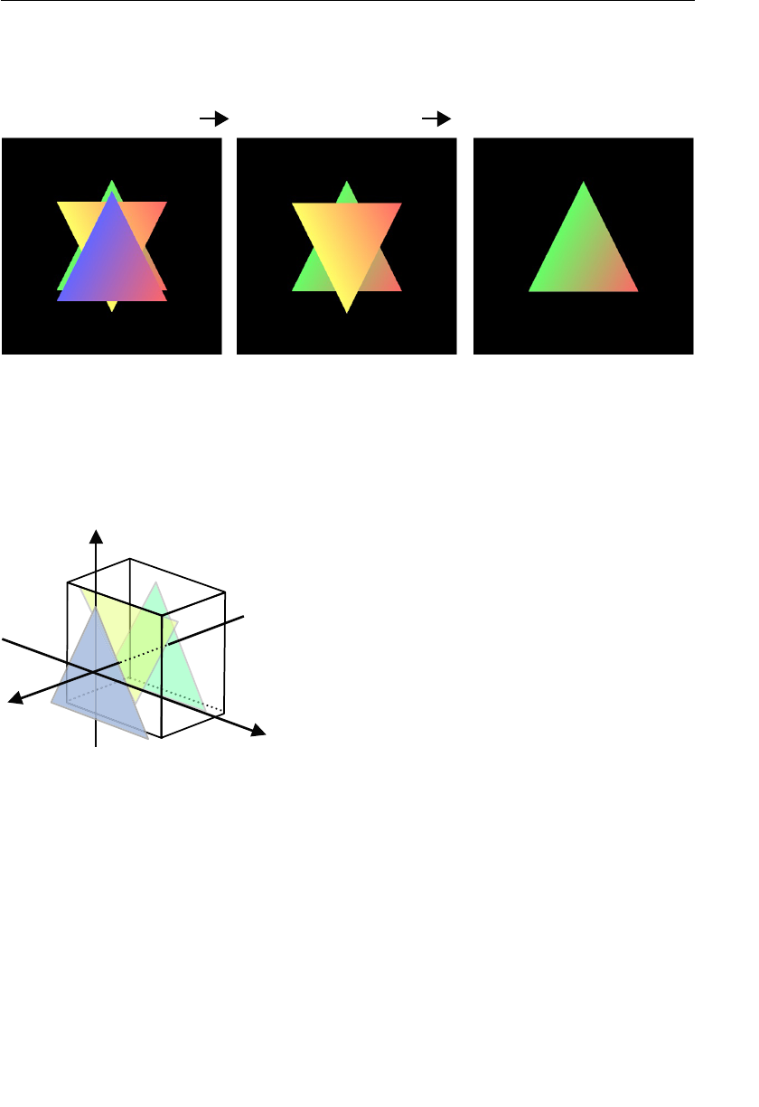
ptg11539634

CHAPTER 7 Toward the 3D World

250

Changing Near or Far

When you run this program and increase the near value (right-arrow key), the display will

change, as shown in Figure 7.14 .

Figure 7.14 Increase the near value using the right arrow key

By default, near is 0.0, so all three triangles are displayed. Next, when you increase near

using the right arrow key, the blue triangle (the front triangle) disappears because the

viewing volume moves past it, as shown in Figure 7.15 . This result is shown as the middle

figure in Figure 7.14 .

Figure 7.15 The blue triangle went outside the viewing volume

Again, if you continue to increase near by pressing the right arrow key, when near becomes

larger than 0.2, the near plane moves past the yellow triangle, so it is outside the viewing

volume and disappears. This leaves only the green triangle (the right figure in Figure 7.14 ).

At this point, if you use the left arrow key to decrease near so it becomes less than 0.2, the

yellow triangle becomes visible again. Alternatively, if you keep on increasing near , the

green triangle will also disappear, leaving the black canvas.

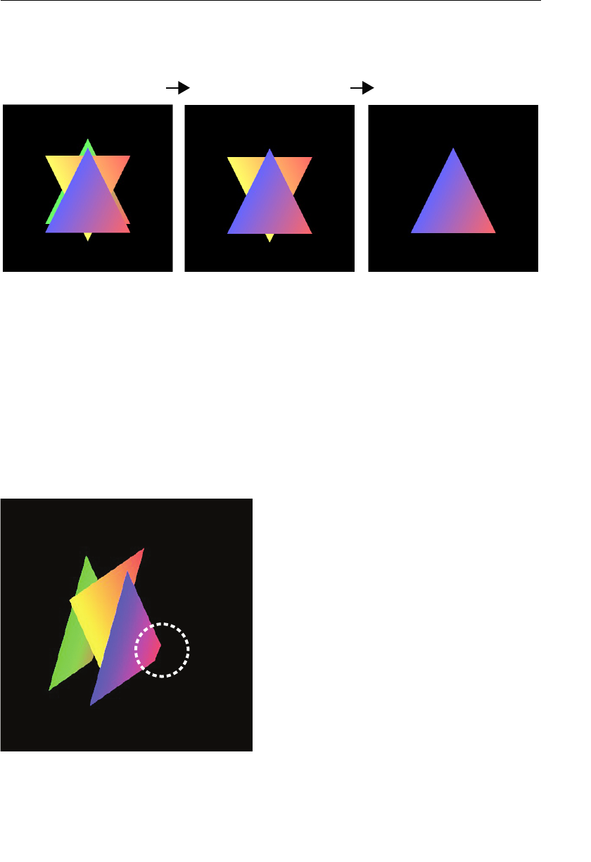
ptg11539634

Specifying the Visible Range (Box Type) 251

As you can imagine, the behavior when you alter the far value is similar. As shown in

Figure 7.16 , when far becomes less than 0.4, the back triangle (the green one) will disap-

pear. Again, if you keep decreasing far , only the blue triangle will remain.

Figure 7.16 Decrease the far value using the down arrow key

This example should clarify the role of the viewing volume. Essentially, for any object you

want to display, you need to place it inside the viewing volume.

Restoring the Clipped Parts of the Triangles

(LookAtTrianglesWithKeys_ViewVolume.js)

In LookAtTrianglesWithKeys , when you kept pressing the arrow keys, part of the triangle

is clipped, as shown in Figure 7.17 . From the previous discussion, it’s clear this is because

some part went outside the viewing volume. In this section, you will modify the sample

program to display the triangle correctly by setting the appropriate viewing volume.

Figure 7.17 A part of the triangle is clipped.

ptg11539634

CHAPTER 7 Toward the 3D World

252

As you can see from the figure, the far corner of the triangle from the eye point is clipped.

Obviously, the far clipping plane is too close to the eye point, so you need to move the far

clipping plane farther out than the current one. To achieve this, you can modify the argu-

ments of the viewing volume so that left =–1.0, right=1.0, bottom =–1.0, top =1.0, near =0.0,

and far =2.0.

You will use two matrices in this program: the matrix that sets the viewing volume (the

orthographic projection matrix), and the matrix that sets the eye point and the line of

sight (view matrix). Because

setOrtho() sets the viewing volume from the eye point, you

need to set the position of the eye point and then set the viewing volume. Consequently,

you will multiply the view matrix by the vertex coordinates to get the vertex coordi-

nates, which are “viewed from the eye position” first, and then multiply the orthographic

projection matrix by the coordinates. You can calculate them as shown in Equation 7.3 .

Equation 7.3

〈〉×〈〉×〈〉orthographic projection matrix view matrix vertex coordinates  

This can be implemented in the vertex shader, as shown in Listing 7.7 .

Listing 7.7 LookAtTrianglesWithKeys_ViewVolume.js

1 // LookAtTrianglesWithKeys_ViewVolume.js

2 // Vertex shader program

3 var VSHADER_SOURCE =

4 ‘attribute vec4 a_Position;n’ +

5 ‘attribute vec4 a_Color;n’ +

6 ‘uniform mat4 u_ViewMatrix;n’ +

7 ‘uniform mat4 u_ProjMatrix;n’ +

8 ‘varying vec4 v_Color;n’ +

9 ‘void main() {n’ +

10 ‘ gl_Position = u_ProjMatrix * u_ViewMatrix * a_Position;n’ +

11 ‘ v_Color = a_Color;n’ +

12 ‘}n’;

…

24 function main() {

…

51 // Get the storage locations of u_ViewMatrix and u_ProjMatrix

52 varu_ViewMatrix = gl.getUniformLocation(gl.program,’u_ViewMatrix’);

53 var u_ProjMatrix = gl.getUniformLocation(gl.program,’u_ProjMatrix’);

…

59 // Create the matrix to specify the view matrix

60 var viewMatrix = new Matrix4();

61 // Register the event handler to be called on key press

62 document.onkeydown = function(ev) { keydown(ev, gl, n, u_ViewMatrix,

➥viewMatrix); };

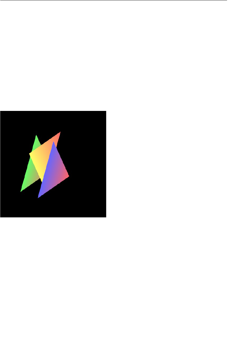
ptg11539634

Specifying the Visible Range (Box Type) 253

64 // Create the matrix to specify the viewing volume and pass it to u_ProjMatrix

65 var projMatrix = new Matrix4();

66 projMatrix.setOrtho(-1.0, 1.0, -1.0, 1.0, 0.0, 2.0);

67 gl.uniformMatrix4fv(u_ProjMatrix, false, projMatrix.elements);

69 draw(gl, n, u_ViewMatrix, viewMatrix); // Draw the triangles

70 }

Line 66 calculates the orthographic projection matrix ( projMatrix ) by modifying far from

1.0 to 2.0. The result matrix is passed to

u_ProjMatrix in the vertex shader at line 67.

A uniform variable is used because the elements in the matrix are uniform for all vertex

coordinates. If you run this sample program and move the eye point as before, you can

see that the triangle no longer gets clipped (see Figure 7.18 ).

Figure 7.18 LookAtTrianglesWithKeys_ViewVolume

Experimenting with the Sample Program

As we explained in the section “Specify the Viewing Volume,” if the aspect ratio of

<canvas> is different from that of the near clipping plane, distorted objects are displayed.

Let’s explore this. First, in

OrthoView_halfSize (based on Listing 7.7 ), you reduce the

current size of the near clipping plane to half while keeping its aspect ratio:

projMatrix.setOrtho(-0.5, 0.5, -0.5, 0.5, 0, 0.5);

The result is shown on the left of Figure 7.19 . As you can see, the triangles appear twice

as large as those of the previous sample because the size of

<canvas> is the same as before.

Note that the parts of the triangles outside the near clipping plane are clipped.

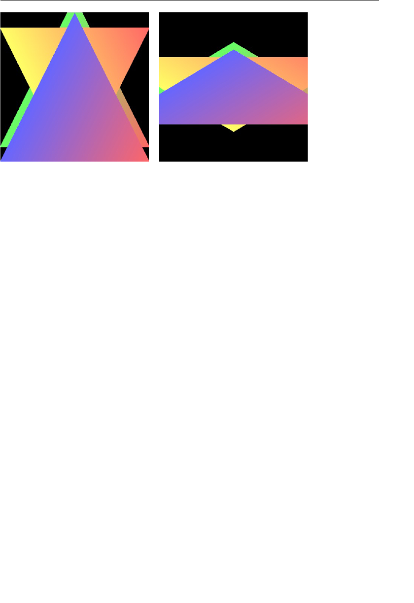
ptg11539634

CHAPTER 7 Toward the 3D World

254

Figure 7.19 Modify the size of the near clipping plane

OrthoView_halfWidth , you reduce only the width of the near clipping plane by chang-

ing the first two arguments in

setOrtho() as follows:

projMatrix.setOrtho(-0.3, 0.3, -1.0, 1.0, 0.0, 0.5);

You can see the results on the right side of Figure 7.19 . This is because the near clipping

plane is horizontally reduced and then horizontally extended (and thus distorted) to fit

the square-shaped

<canvas> when the plane is displayed.

Specifying the Visible Range Using a Quadrangular

Pyramid

Figure 7.20 shows a tree-lined road scene. In this picture, all the trees on the left and right

sides are approximately of the same height, but the farther back they are, the smaller

they look. Equally, the building in the distance appears smaller than the trees that are

closer to the viewer, even though the building is actually taller than the trees. This effect

of distant objects looking smaller gives the feeling of depth. Although our eyes perceive

reality in this way, it’s interesting to notice that children’s drawings rarely show this kind

of perspective.

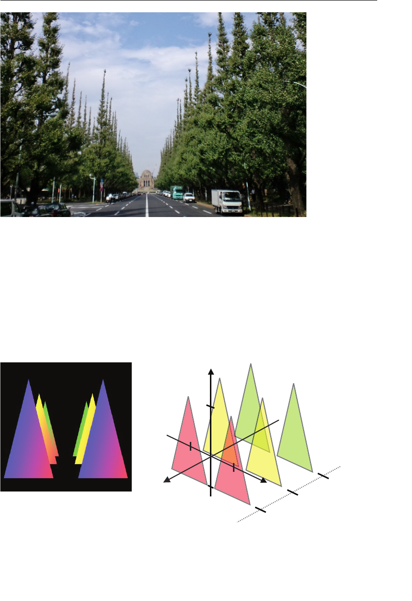
ptg11539634

Specifying the Visible Range Using a Quadrangular Pyramid 255

Figure 7.20 Tree-lined road

In the case of the box-shaped viewing volume explained in the previous section, identi-

cally sized triangles are drawn the same size, regardless of their distance from the eye

point. To overcome this constraint, you can use the quadrangular pyramid viewing

volume, which allows you to give this sense of depth, as seen in Figure 7.20 .

Here you construct the sample program

PerspectiveView , which sets a quadrangular

pyramid viewing volume that points along the negative z-axis from the eye point set at

(0, 0, 5). Figure 7.21 shows a screen shot of

PerspectiveView and the location of each

triangle.

-0.75

0.75

1.0

-1.0

0.0

-2.0

-4.0

Figure 7.21 PerspectiveView; location of each triangle

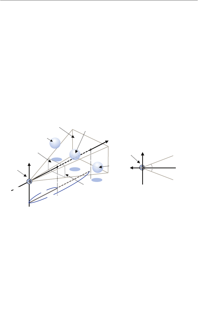
ptg11539634

CHAPTER 7 Toward the 3D World

256

As can be seen from the figure on the right, three identically sized triangles are positioned

on the right and left sides along the coordinate’s axes, in a way similar to the tree-lined

road. By using a quadrangular pyramid viewing volume, WebGL can automatically display

remote objects as if they are smaller, thus achieving the sense of depth. This is shown in

the left side of the figure.

To really notice the change in size, as in the real world, the objects need to be located

at a substantial distance. For example, when looking at the box, to actually make the

background area looks smaller than the foreground area, this box needs to have consider-

able depth. So this time, you will use a slightly more distant position (0, 0, 0.5) than the

default value (0, 0, 0) for the eye point.

Setting the Quadrangular Pyramid Viewing Volume

The quadrangular pyramid viewing volume is shaped as shown in Figure 7.22 . Just like

the box-shaped configuration, the viewing volume is set at the eye point along the line of

sight, and objects located between the far and near clipping planes are displayed. Objects

positioned outside the viewing volume are not shown, while those straddling the bound-

ary will only have parts located inside the viewing volume visible.

vof

raen

raf

eye point

vector

near clipping plane

far clipping plane

aspect

(aspect of near clipping plane)

invisible

visible

line of sight

Figure 7.22 Quadrangular pyramid viewing volume

Regardless of whether it is a quadrangular pyramid or a box, you set the viewing volume

using matrices, but the arguments differ. The

Matrix4 ’s method setPerspective() is used

to configure the quadrangular pyramid viewing volume.

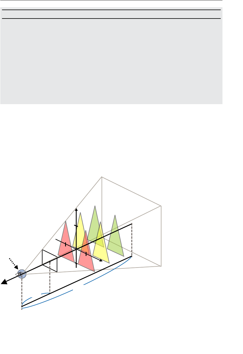
ptg11539634

Specifying the Visible Range Using a Quadrangular Pyramid 257

Matrix4.setPerspective(fov, aspect, near, far)

Calculate the matrix (the perspective projection matrix) that defines the viewing volume

specified by its arguments, and store it in

Matrix4 . However, the near value must be less

than the far value .

Parameters fov Specifies field of view, angle formed by the top and bottom

planes. It must be greater than 0 .

aspect Specifies the aspect ratio of the near plane (width/height).

near, far Specify the distances to the near and far clipping planes along the

line of sight ( near > 0 and far > 0).

Return value None

The matrix that sets the quadrangular pyramid viewing volume is called the perspective

projection matrix .

Note that the specification for the near plane is different from that of the box type with

the second argument, aspect, representing the near plane aspect ratio. For example, if we

set the height to 100 and the width to 200, the aspect ratio is 0.5.

The positioning of the triangles with regard to the viewing volume we are using is illus-

trated in Figure 7.23 . It is specified by near =1.0, far =100, aspect =1.0 (the same aspect ratio

as the canvas), and fov =30.0.

eye point

(0, 0, 5)

(0, 0, 4)

near = 1

far=100

-0.75

0.75

1.0

-1.0

Figure 7.23 The positions of the triangles with respect to the quadrangular pyramid viewing

volume

ptg11539634

CHAPTER 7 Toward the 3D World

258

The basic processing flow is similar to that of LookAtTrianglesWithKeys_ViewVolume.js in

the previous section. So let’s take a look at the sample program.

Sample Program (PerspectiveView.js)

The sample program is detailed in Listing 7.8 .

Listing 7.8 PerspectiveView.js

1 // PerspectiveView.js

2 // Vertex shader program

3 var VSHADER_SOURCE =

4 ‘attribute vec4 a_Position;n’ +

5 ‘attribute vec4 a_Color;n’ +

6 ‘uniform mat4 u_ViewMatrix;n’ +

7 ‘uniform mat4 u_ProjMatrix;n’ +

8 ‘varying vec4 v_Color;n’ +

9 ‘void main() {n’ +

10 ‘ gl_Position = u_ProjMatrix * u_ViewMatrix * a_Position;n’ +

11 ‘ v_Color = a_Color;n’ +

12 ‘}n’;

…

24 function main() {

…

41 // Set the vertex coordinates and color (blue triangle is in front)

42 var n = initVertexBuffers(gl);

…

51 // Get the storage locations of u_ViewMatrix and u_ProjMatrix

52 varu_ViewMatrix = gl.getUniformLocation(gl.program,’u_ViewMatrix’);

53 var u_ProjMatrix = gl.getUniformLocation(gl.program,’u_ProjMatrix’);

…

59 var viewMatrix = new Matrix4(); // The view matrix

60 var projMatrix = new Matrix4(); // The projection matrix

62 // Calculate the view and projection matrix

63 viewMatrix.setLookAt(0, 0, 5, 0, 0, -100, 0, 1, 0);

64 projMatrix.setPerspective(30, canvas.width/canvas.height, 1, 100);

65 // Pass The view matrix and projection matrix to u_ViewMatrix and u_ProjMatrix

66 gl.uniformMatrix4fv(u_ViewMatrix, false, viewMatrix.elements);

67 gl.uniformMatrix4fv(u_ProjMatrix, false, projMatrix.elements);

…

72 // Draw the rectangles

73 gl.drawArrays(gl.TRIANGLES, 0, n);

74 }

ptg11539634

Specifying the Visible Range Using a Quadrangular Pyramid 259

76 function initVertexBuffers(gl) {

77 var verticesColors = new Float32Array([

78 // Three triangles on the right side

79 0.75, 1.0, -4.0, 0.4, 1.0, 0.4, // The green triangle in back

80 0.25, -1.0, -4.0, 0.4, 1.0, 0.4,

81 1.25, -1.0, -4.0, 1.0, 0.4, 0.4,

83 0.75, 1.0, -2.0, 1.0, 1.0, 0.4, // The yellow triangle in middle

84 0.25, -1.0, -2.0, 1.0, 1.0, 0.4,

85 1.25, -1.0, -2.0, 1.0, 0.4, 0.4,

87 0.75, 1.0, 0.0, 0.4, 0.4, 1.0, // The blue triangle in front

88 0.25, -1.0, 0.0, 0.4, 0.4, 1.0,

89 1.25, -1.0, 0.0, 1.0, 0.4, 0.4,

91 // Three triangles on the left side

92 -0.75, 1.0, -4.0, 0.4, 1.0, 0.4, // The green triangle in back

93 -1.25, -1.0, -4.0, 0.4, 1.0, 0.4,

94 -0.25, -1.0, -4.0, 1.0, 0.4, 0.4,

96 -0.75, 1.0, -2.0, 1.0, 1.0, 0.4, // The yellow triangle in middle

97 -1.25, -1.0, -2.0, 1.0, 1.0, 0.4,

98 -0.25, -1.0, -2.0, 1.0, 0.4, 0.4,

100 -0.75, 1.0, 0.0, 0.4, 0.4, 1.0, // The blue triangle in front

101 -1.25, -1.0, 0.0, 0.4, 0.4, 1.0,

102 -0.25, -1.0, 0.0, 1.0, 0.4, 0.4,

103 ]);

104 var n = 18; // Three vertices per triangle * 6

…

138 return n;

139 }

The vertex and fragment shaders are completely identical (including the names of the

variables) to the ones used in

LookAtTriangles_ViewVolume.js .

The processing flow of main() in JavaScript is also similar. Calling initVertexBuffers()

at line 42 writes the vertex coordinates and colors of the six triangles to be displayed into

the buffer object. In

initVertexBuffers() , the vertex coordinates and colors for the six

triangles are specified: three triangles positioned on the right side from line 79 and three

triangles positioned on the left side from line 92. As a result, the number of vertices to be

drawn at line 104 is changed to 18 (3×6=18, to handle six triangles).

At lines 52 and 53 in

main() , the locations of the uniform variables that store the view

matrix and perspective projection matrix are retrieved. Then at line 59 and 60, the vari-

ables used to hold the matrices are created.

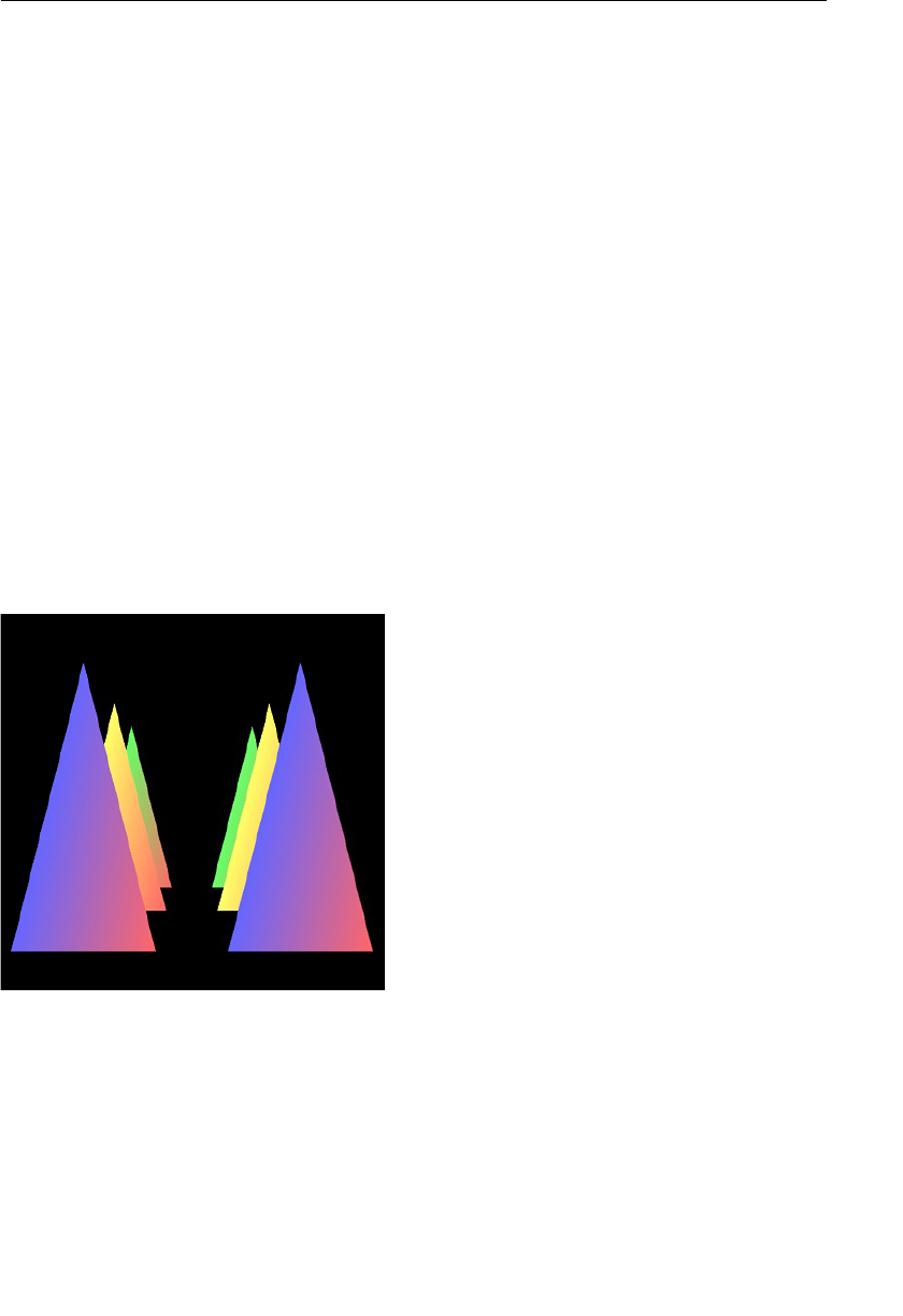
ptg11539634

CHAPTER 7 Toward the 3D World

260

At line 63, the view matrix is calculated, with the eye point set at (0, 0, 5), the line of

sight set along the z-axis in the negative direction, and the up direction set along the

y-axis in the positive direction. Finally at line 64, the projection matrix is set up using a

quadrangular pyramid viewing volume:

64 projMatrix.setPerspective(30, canvas.width/canvas.height, 1, 100);

The second argument aspect (the horizontal to vertical ratio of the near plane) is derived

from the

<canvas> width and height ( width and height property), so any modification of

the

<canvas> aspect ratio doesn’t lead to distortion of the objects displayed.

Next, as the view and perspective projection matrices are available, you pass them to the

appropriate uniform variables at lines 66 and 67. Finally, you draw the triangles at line 73,

and upon execution you get a result including perspective similar to that shown in Figure

7.20 .

Finally, one aspect touched on earlier but not fully explained is why matrices are used to

set the viewing volume. Without using mathematics, let’s explore that a little.

The Role of the Projection Matrix

Let’s start by examining the perspective projection matrix. Looking at the screen shot of

PerspectiveView in Figure 7.24 , you can see that, after applying the projection matrix, the

objects in the distance are altered in two ways.

Figure 7.24 PerspectiveView

First, the farther away the triangles are, the smaller they appear. Second, the triangles are

parallel shifted so they look as if they are positioned inward toward the line of sight. In

comparison to the identically sized triangles that are laid out as shown on the left side

of Figure 7.25 , the following two transformations have been applied: (1) triangles farther

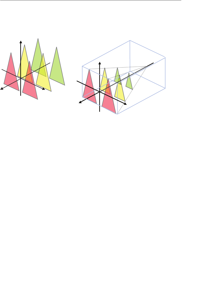
ptg11539634

Specifying the Visible Range Using a Quadrangular Pyramid 261

from the viewer are scaled down (transformed) in proportion to the distance from the

viewer, and (2) the triangles are then transformed to be shifted toward the line of sight, as

illustrated on the right side of Figure 7.25 . These two transformations, shown on the right

side of Figure 7.25 , enable the effect you see in the photograph scene shown in Figure

7.20 .

point at

infinity

Figure 7.25 Conceptual rendering of the perspective projection transformation

This means that the specification of the viewing volume can be represented as a combina-

tion of transformations, such as the scaling or translation of geometric shapes and objects,

in accordance with the shape of the viewing volume. The Matrix4 object’s method

setPerspective() automatically calculates this transformation matrix from the arguments

of the specified viewing volume. The elements of the matrix are discussed in Appendix C ,

“Projection Matrices.” If you are interested in the mathematical explanation of the coordi-

nate transform related to the viewing volume, please refer to the book Computer Graphics .

To put it another way, the transformation associated with the perspective projection trans-

forms the quadrangular pyramid viewing volume into a box-shaped viewing volume (right

part of Figure 7.25 ).

Note that the orthographic projection matrix does not perform all the work needed for

this transformation to generate the required optical effect. Rather, it performs the prelimi-

nary preparation that is required by the post vertex shader processing—where the actual

processing is done. If you are interested in this, please refer to Appendix D , “WebGL/

OpenGL: Left or Right Handed?”

The projection matrix, combined with the model matrix and the view matrix, is able

to handle all the necessary geometric transformations (translation, rotation, scaling) for

achieving the different optical effects. The following section will explore how to combine

these matrices to do that using a simple example.

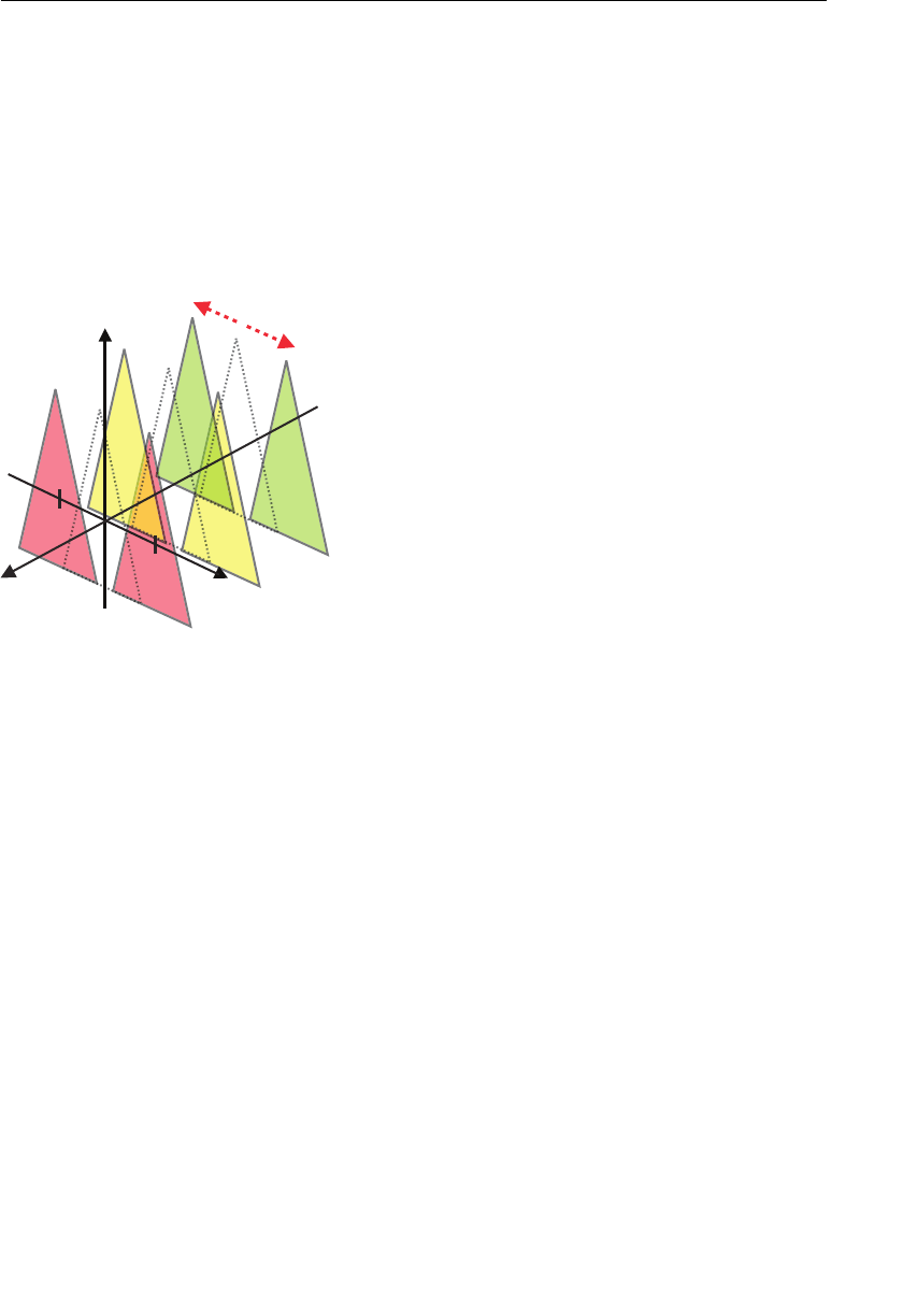
ptg11539634

CHAPTER 7 Toward the 3D World

262

Using All the Matrices (Model Matrix, View Matrix, and Projection

Matrix)

One of the issues with PerspectiveView.js is the amount of code needed to set up the

vertex coordinates and the color data. Because we only have to deal with six triangles in

this case, it’s still manageable, but it could get messy if the number of triangles increased.

Fortunately, there is an effective drawing technique to handle this problem.

If you take a close look at the triangles, you will notice that the configuration is identical

to that in Figure 7.26 , where the dashed triangles are shifted along the x-axis in the posi-

tive (0.75) and negative (–0.75) directions, respectively.

-0.75

0.75

Figure 7.26 Drawing after translation

Taking advantage of this, it is possible to draw the triangles in

PerspectiveView in the

following way:

1. Prepare the vertex coordinates data of the three triangles that are laid out centered

along the z-axis.

2. Translate the original triangles by 0.75 units along the x-axis, and draw them.

3. Translate the original triangles by –0.75 units along the x-axis, and draw them.

Now let’s try to use this approach in some sample code (

PerspectiveView_mvp) .

In the original PerspectiveView program the projection and view matrices were used to

specify the viewer’s viewpoint and viewing volume and

PerspectiveView_mvp , the model

matrix, was used to perform the translation of the triangles.

At this point, it’s worthwhile to review the actions these matrices perform. To do that,

let’s refer to

LookAtTriangles , which you wrote earlier to allow the viewer to look at a

rotated triangle from a specific location. At that time, you used this expression, which is

identical to Equation 7.1 :

ptg11539634

Specifying the Visible Range Using a Quadrangular Pyramid 263

〈〉×〈〉×〈〉view matrix model matrix vertex coordinates

Building on that, in

LookAtTriangles_ViewVolume , which correctly displays the clipped

triangle, you used the following expression, which, when you use projection matrix

to include either orthographic projection or perspective projection, is identical to

Equation 7.3 :

〈〉×〈〉×〈〉projection matrix view matrix vertex coordinates 

You can infer the following from these two expressions:

Equation 7.4

〈〉×〈〉×〈〉×〈〉projection matrix view matrix model matrix vertex coordinates  

This expression shows that, in WebGL, you can calculate the final vertex coordinates

by using three types of matrices: the model matrix, the view matrix, and the projection

matrix.

This can be understood by considering that Equation 7.1 is identical to Equation 7.4 , in

which the projection matrix becomes the identity matrix, and Equation 7.3 is identical

to Equation 7.4 , whose model matrix is turned into the identity matrix. As explained in

Chapter 4 , the identity matrix behaves for matrix multiplication like the scalar 1 does with

scalar multiplication. Multiplying by the identity matrix has no effect on the other matrix.

So let’s construct the sample program using Equation 7.4 .

Sample Program (PerspectiveView_mvp.js)

PerspectiveView_mvp.js is shown in Listing 7.9 . The basic processing flow is similar to

that of

PerspectiveView.js . The only difference is the modification of the calculation in

the vertex shader (line 11) to implement Equation 7.4 , and the passing of the additional

matrix (

u_ModelMatrix ) used for the calculation.

Listing 7.9 PerspectiveView_mvp.js

1 // PerspectiveView_mvp.js

2 // Vertex shader program

3 var VSHADER_SOURCE =

4 ‘attribute vec4 a_Position;n’ +

5 ‘attribute vec4 a_Color;n’ +

6 ‘uniform mat4 u_ModelMatrix;n’ +

7 ‘uniform mat4 u_ViewMatrix;n’ +

8 ‘uniform mat4 u_ProjMatrix;n’ +

9 ‘varying vec4 v_Color;n’ +

10 ‘void main() {n’ +

11 ‘ gl_Position = u_ProjMatrix * u_ViewMatrix * u_ModelMatrix * a_Position;n’ +

12 ‘ v_Color = a_Color;n’ +

ptg11539634

CHAPTER 7 Toward the 3D World

264

13 ‘}n’;

…

25 function main() {

…

42 // Set the vertex coordinates and color (blue triangle is in front)

43 var n = initVertexBuffers(gl);

…

52 // Get the storage locations of u_ModelMatrix, u_ViewMatrix, and u_ProjMatrix.

53 var u_ModelMatrix = gl.getUniformLocation(gl.program, ‘u_ModelMatrix’);

54 var u_ViewMatrix = gl.getUniformLocation(gl.program,’u_ViewMatrix’);

55 var u_ProjMatrix = gl.getUniformLocation(gl.program,’u_ProjMatrix’);

…

61 var modelMatrix = new Matrix4(); // Model matrix

62 var viewMatrix = new Matrix4(); // View matrix

63 var projMatrix = new Matrix4(); // Projection matrix

65 // Calculate the model matrix, view matrix, and projection matrix

66 modelMatrix.setTranslate(0.75, 0, 0); // Translate 0.75 units

67 viewMatrix.setLookAt(0, 0, 5, 0, 0, -100, 0, 1, 0);

68 projMatrix.setPerspective(30, canvas.width/canvas.height, 1, 100);

69 // Pass the model, view, and projection matrix to uniform variables.

70 gl.uniformMatrix4fv(u_ModelMatrix, false, modelMatrix.elements);

71 gl.uniformMatrix4fv(u_ViewMatrix, false, viewMatrix.elements);

72 gl.uniformMatrix4fv(u_ProjMatrix, false, projMatrix.elements);

74 gl.clear(gl.COLOR_BUFFER_BIT);// clear <canvas>

76 gl.drawArrays(gl.TRIANGLES, 0, n); // Draw triangles on right

78 // Prepare the model matrix for another pair of triangles

79 modelMatrix.setTranslate(-0.75, 0, 0); // Translate -0.75

80 // Modify only the model matrix

81 gl.uniformMatrix4fv(u_ModelMatrix, false, modelMatrix.elements);

83 gl.drawArrays(gl.TRIANGLES, 0, n);// Draw triangles on left

84 }

86 function initVertexBuffers(gl) {

87 var verticesColors = new Float32Array([

88 // Vertex coordinates and color

89 0.0, 1.0, -4.0, 0.4, 1.0, 0.4, // The back green triangle

90 -0.5, -1.0, -4.0, 0.4, 1.0, 0.4,

91 0.5, -1.0, -4.0, 1.0, 0.4, 0.4,

93 0.0, 1.0, -2.0, 1.0, 1.0, 0.4, // The middle yellow triangle

ptg11539634

Specifying the Visible Range Using a Quadrangular Pyramid 265

94 -0.5, -1.0, -2.0, 1.0, 1.0, 0.4,

95 0.5, -1.0, -2.0, 1.0, 0.4, 0.4,

97 0.0, 1.0, 0.0, 0.4, 0.4, 1.0, // The front blue triangle

98 -0.5, -1.0, 0.0, 0.4, 0.4, 1.0,

99 0.5, -1.0, 0.0, 1.0, 0.4, 0.4,

100 ]);

…

135 return n;

136 }

This time, you need to pass the model matrix to the vertex shader, so u_ModelMatrix is

added at line 6. The matrix is used at line 11, which implements Equation 7.5:

11 ‘ gl_Position = u_ProjMatrix * u_ViewMatrix * u_ModelMatrix * a_Position;n’ +

Next, main() in JavaScript calls initVertexBuffers() at line 43. In this function, the

vertex coordinates of the triangles to be passed to the buffer object are defined (line 87).

This time, you are handling the vertex coordinates of three triangles centered along the

z-axis instead of the six triangles used in

PerspectiveView.js . As mentioned before, this is

because you will use the three triangles in conjunction with a translation.

At line 53, the storage location of

u_ModelMatrix in the vertex shader is obtained. At

line 61, the arguments for the matrix (

modelMatrix ) passed to the uniform variable are

prepared, and at line 66, the matrix is calculated. First, this matrix will translate the trian-

gles by 0.75 units along the x-axis:

65 // Calculate the view matrix and the projection matrix

66 modelMatrix.setTranslate(0.75, 0, 0); // Translate 0.75

…

70 gl.uniformMatrix4fv(u_ModelMatrix, false, modelMatrix.elements);

…

76 gl.drawArrays(gl.TRIANGLES, 0, n); // Draw a triangle

The matrix calculations, apart from the model matrix at line 66, are the same as in

PerspectiveView.js . The model matrix is passed to u_ModelMatrix at line 70 and used to

draw the right side row of triangles (line 76).

In a similar manner, the row of triangles for the left side is translated by –0.75 units along

the x-axis, and then the model matrix is calculated again at line 79. Because the view

matrix and projection matrix make use of this model matrix, you only need to assign

the model matrix to the uniform variable once (line 81). Once the matrix is set up, you

perform the draw operation at line 83 with

gl.drawArrays() :

78 // Prepare the model matrix for another pair of triangles

79 modelMatrix.setTranslate(-0.75, 0, 0); // Translate -0.75

80 // Modify only the model matrix

ptg11539634

CHAPTER 7 Toward the 3D World

266

81 gl.uniformMatrix4fv(u_ModelMatrix, false, modelMatrix.elements);

83 gl.drawArrays(gl.TRIANGLES, 0, n); // Draw triangles on left

As you have seen, this approach allows you to draw two sets of triangles from a single set

of triangle data, which reduces the number of vertices needed but increases the number

of calls to

gl.drawArrays() . The choice of which approach to use for better performance

depends on the application and the WebGL implementation.

Experimenting with the Sample Program

In PerspectiveView_mvp , you calculated

ection matrix view matrix model matrix 

directly inside the vertex shader. This calculation of is the same for all the vertices, so

there is no need to recalculate it inside the shader for each vertex. It can be computed in

advance inside the JavaScript code, as it was in

LookAtRotatedTriangles_mvMatrix earlier

in the chapter, allowing a single matrix to be passed to the vertex shader. This matrix is

called the model view projection matrix , and the name of the variable that passes it is

u_MvpMatrix . The sample program used to show this is ProjectiveView_mvpMatrix , in

which the vertex shader is modified as shown next and, as you can see, is significantly

simpler:

1 // PerspectiveView_mvpMatrix.js

2 // Vertex shader program

3 var VSHADER_SOURCE =

4 ‘attribute vec4 a_Position;n’ +

5 ‘attribute vec4 a_Color;n’ +

6 ‘uniform mat4 u_MvpMatrix;n’ +

7 ‘varying vec4 v_Color;n’ +

8 ‘void main() {n’ +

9 ‘ gl_Position = u_MvpMatrix * a_Position;n’ +

10 ‘ v_Color = a_Color;n’ +

11 ‘}n’;

In JavaScript, main() , the storage location of u_ModelMatrix is retrieved at line 51, and

then the matrix to be stored in the uniform variable is calculated at line 57:

50 // Get the storage location of u_MvpMatrix

51 var u_MvpMatrix = gl.getUniformLocation(gl.program, ‘u_MvpMatrix’);

…

57 var modelMatrix = new Matrix4(); // The model matrix

58 var viewMatrix = new Matrix4(); // The view matrix

ptg11539634

Correctly Handling Foreground and Background Objects 267

59 var projMatrix = new Matrix4(); // The projection matrix

60 var mvpMatrix = new Matrix4(); // The model view projection matrix

62 // Calculate the model, view, and projection matrices

63 modelMatrix.setTranslate(0.75, 0, 0);

64 viewMatrix.setLookAt(0, 0, 5, 0, 0, -100, 0, 1, 0);

65 projMatrix.setPerspective(30, canvas.width/canvas.height, 1, 100);

66 // Calculate the model view projection matrix

67 mvpMatrix.set(projMatrix).multiply(viewMatrix).multiply(modelMatrxi);

68 // Pass the model view projection matrix to u_MvpMatrix

69 gl.uniformMatrix4fv(u_MvpMatrix, false, mvpMatrix.elements);

…

73 gl.drawArrays(gl.TRIANGLES, 0, n); // Draw a rectangle

75 // Prepare the model matrix for another pair of triangles

76 modelMatrix.setTranslate(-0.75, 0, 0);

77 // Calculate the model view projection matrix

78 mvpMatrix.set(projMatrix).multiply(viewMatrix).multiply(modelMatrxi);

79 // Pass the model view projection matrix to u_MvpMatrix

80 gl.uniformMatrix4fv(u_MvpMatrix, false, mvpMatrix.elements);

82 gl.drawArrays(gl.TRIANGLES, 0, n); // Draw a rectangle

83 }

The critical calculation is carried out at line 67. The projection matrix ( projMatrix ) is

assigned to

mvpMatrix . Then the view matrix ( viewMatrix ) is multiplied by the model

matrix (

modelMatrix ), and the result is written back to mvpMatrix , using the set version

of the method. This is in turn assigned to

u_MvpMatrix at line 69, and the triangles on

the right side are drawn at line 73. Similarly, the calculation of the model view projec-

tion matrix for the triangles on the left side is performed at line 78. It is then passed to

u_MvpMatrix at line 80, and the triangles are drawn at line 82.

With this information, you are now able to write code that moves the eye point, sets the

viewing volume, and allows you to view three-dimensional objects from various angles.

Additionally, you have learned how to deal with clipping that resulted in partially missing

objects. However, one potential problem remains. As you move the eye point to a differ-

ent location, it’s possible for objects in the foreground to be hidden by objects in the

background. Let’s look at how this problem comes about.

Correctly Handling Foreground and Background

Objects

In the real world, if you place two boxes on a desk as shown in Figure 7.27 , the fore-

ground box partially hides the background one.

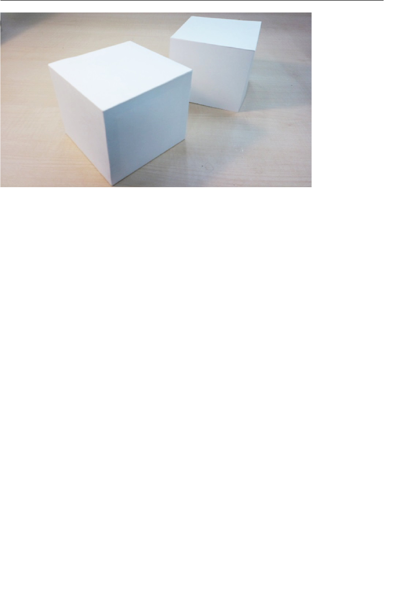
ptg11539634

CHAPTER 7 Toward the 3D World

268

Figure 7.27 The front object partially hides the back object

Looking at the sample programs constructed so far, such as the screen shot of

PerspectiveView (refer to Figure 7.21 ), the green triangle located at the back is partially

hidden by the yellow and blue triangles. It looks as if WebGL, being designed for display-

ing 3D objects, has naturally figured out the correct order.

However, that is unfortunately not the case. By default, WebGL, to accelerate the drawing

process, draws objects in the order of the vertices specified inside the buffer object. Up

until now, you have always arranged the order of the vertices so that the objects located

in the background are drawn first, thus resulting in a natural rendering.

For example, in

PerspectiveView_mvpMatrix.js , you specified the coordinates and color

of the triangles in the following order. Note the z coordinates (bold font):

var verticesColors = new Float32Array([

// vertex coordinates and color

0.0, 1.0, -4.0 , 0.4, 1.0, 0.4, // The green one at the back

-0.5, -1.0, -4.0 , 0.4, 1.0, 0.4,

0.5, -1.0, -4.0 , 1.0, 0.4, 0.4,

0.0, 1.0, -2.0 , 1.0, 1.0, 0.4, // The yellow one in the middle

-0.5, -1.0, -2.0 , 1.0, 1.0, 0.4,

0.5, -1.0, -2.0 , 1.0, 0.4, 0.4,

0.0, 1.0, 0.0 , 0.4, 0.4, 1.0, // The blue one in the front

-0.5, -1.0, 0.0 , 0.4, 0.4, 1.0,

0.5, -1.0, 0.0 , 1.0, 0.4, 0.4,

]);

WebGL draws the triangles in the order z in which you specified the vertices (that is,

the green triangle [back], then the yellow triangle [middle], and finally the blue triangle

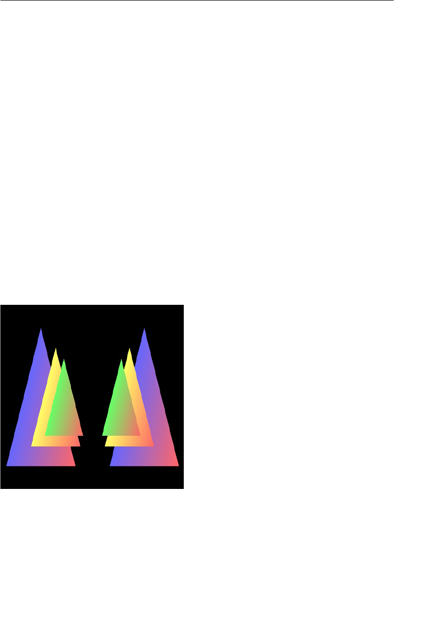
ptg11539634

Correctly Handling Foreground and Background Objects 269

[front]). This ensures that objects closer to the eye point cover those farther away, as seen

in Figure 7.13 .

To verify this, let’s modify the order in which the triangles are specified by first drawing

the blue triangle in the front, then the yellow triangle in the middle, and finally the green

triangle at the back:

var verticesColors = new Float32Array([

// vertex coordinates and color

0.0, 1.0, 0.0, 0.4, 0.4, 1.0, // The blue one in the front

-0.5, -1.0, 0.0, 0.4, 0.4, 1.0,

0.5, -1.0, 0.0, 1.0, 0.4, 0.4

0.0, 1.0, -2.0, 1.0, 1.0, 0.4, // The yellow one in the middle

-0.5, -1.0, -2.0, 1.0, 1.0, 0.4,

0.5, -1.0, -2.0, 1.0, 0.4, 0.4,

0.0, 1.0, -4.0, 0.4, 1.0, 0.4, // The green one at the back

-0.5, -1.0, -4.0, 0.4, 1.0, 0.4,

0.5, -1.0, -4.0, 1.0, 0.4, 0.4,

]);

When you run this, you’ll see the green triangle, which is supposed to be located at the

back, has been drawn at the front (see Figure 7.28 ).

Figure 7.28 The green triangle in the back is displayed at the front

Drawing objects in the specified order, the default behavior in WebGL, can be quite

efficient when the sequence can be determined beforehand and the scene doesn’t

ptg11539634

CHAPTER 7 Toward the 3D World

270

subsequently change. However, when you examine the object from various directions by

moving the eye point, it is impossible to decide the drawing order in advance.

Hidden Surface Removal

To cope with this problem, WebGL provides a hidden surface removal function. This

function eliminates surfaces hidden behind foreground objects, allowing you to draw the

scene so that the objects in the back are properly hidden by those in front, regardless of

the specified vertex order. This function is already embedded in WebGL and simply needs

to be enabled.

Enabling hidden surface removal and preparing WebGL to use it requires the following

two steps:

1. Enabling the hidden surface removal function

gl.enable(gl.DEPTH_TEST);

2. Clearing the depth buffer used for the hidden surface removal before drawing

gl.clear(gl.DEPTH_BUFFER_BIT);

The function gl.enable() , used in step 1, actually enables various functions in WebGL.

gl.enable(cap)

Enable the function specified by cap (capability).

Parameters cap Specifies the function to be

enabled.

gl.DEPTH_TEST

2 Hidden surface removal

gl.BLEND Blending (see Chapter 9 ,

“Hierarchical Objects”)

gl.POLYGON_OFFSET_FILL Polygon offset (see the next

section), and so on

Return value None

Errors : INVALID_ENUM None of the acceptable values is specified in cap

3 Although not covered in this book, you can also specify gl.CULL_FACE , gl.DITHER , gl.SAMPLE_

ALPHA_TO_COVERAGE , gl.SAMPLE_COVERAGE , gl.SCISSOR_TEST , and gl.STENCIL_TEST . See the

book OpenGL Programming Guide for more information on these.

2 A “DEPTH_TEST” in the hidden surface removal function might sound strange, but actually its name

comes from the fact that it decides which objects to draw in the foreground by verifying (TEST) the

depth (DEPTH) of each object.

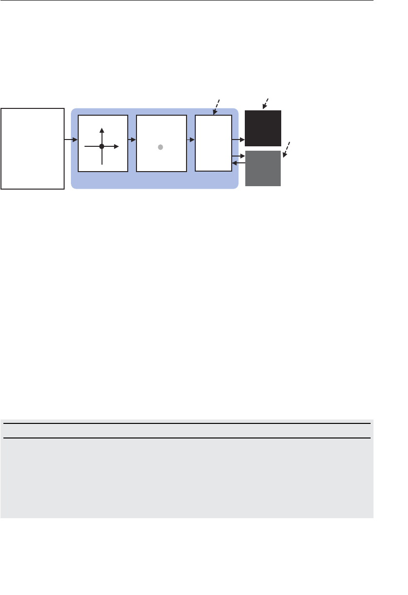
ptg11539634

Correctly Handling Foreground and Background Objects 271

The depth buffer cleared in the gl.clear() statement (step 2) is a buffer used internally

to remove hidden surfaces. While WebGL draws objects and geometric shapes in the color

buffer displayed on the

<canvas> , hidden surface removal requires the depth (from the

eye point) for each geometrical shape and object. The depth buffer holds this information

(see Figure 7.29 ). The depth direction is the same as the z-axis direction, so it is sometimes

called the z-buffer.

metsySLGbeW

redahSxetreV

tpircSavaJ

{)(niamnoitcnuf

…LGbeWteg=lgrav

…

;)…(sredahStini

…

}

y reffuBhtpeD

htpeD

tseT

lavomeRecafruSneddiHreffuBroloC

tnemgarF

redahS

Figure 7.29 Depth buffer used in hidden surface removal

Because the depth buffer is used whenever a drawing command is issued, it must be

cleared before any drawing operation; otherwise, you will see incorrect results. You specify

the depth buffer using

gl.DEPTH_BUFFER_BIT and proceed as follows to clear it:

gl.clear(gl.DEPTH_BUFFER_BIT);

Up until now, you only cleared the color buffer. Because you now need to also clear the

depth buffer, you can clear both buffers simultaneously by taking the bitwise or (|) of

gl.COLOR_BUFFER_BIT (which represents the color buffer) and gl.DEPTH_BUFFER_BIT

(which represents the depth buffer) and specifying it as an argument to

gl.clear() :

gl.clear(gl.COLOR_BUFFER_BIT | gl.DEPTH_BUFFER_BIT);

You can use the bitwise or operation this way whenever you need to clear both buffers at

the same time.

To disable the function you enabled with

gl.enable() , you use gl.disable() .

gl.disable(cap)

Disable the function specified by cap (capability).

Parameters cap Same as

gl.enable() .

Return value None

Errors INVALID_ENUM None of the acceptable values is specified in cap

ptg11539634

CHAPTER 7 Toward the 3D World

272

Sample Program (DepthBuffer.js)

Let’s add the hidden surface removal methods from (1) and (2) to PerspectiveView_

mvpMatrix.js and change the name to DepthBuffer.js . Note that the order of the vertex

coordinates specified inside the buffer object is not changed, so you will draw from

front to back the blue, yellow, and green triangles. The result is identical to that of the

PerspectiveView_mvpMatrix . We detail the program in Listing 7.10 .

Listing 7.10 DepthBuffer.js

1 // DepthBuffer.js

…

23 function main() {

…

41 var n = initVertexBuffers(gl);

…

47 // Specify the color for clearing <canvas>

48 gl.clearColor(0, 0, 0, 1);

49 // Enable the hidden surface removal function

50 gl.enable(gl.DEPTH_TEST);

73 // Clear the color and depth buffer

74 gl.clear(gl.COLOR_BUFFER_BIT | gl.DEPTH_BUFFER_BIT);

76 gl.drawArrays(gl.TRIANGLES, 0, n); // Draw triangles

…

85 gl.drawArrays(gl.TRIANGLES, 0, n); // Draw triangles

86 }

88 function initVertexBuffers(gl) {

89 var verticesColors = new Float32Array([

90 // Vertex coordinates and color

91 0.0, 1.0, 0.0, 0.4, 0.4, 1.0, // The blue triangle in front

92 -0.5, -1.0, 0.0, 0.4, 0.4, 1.0,

93 0.5, -1.0, 0.0, 1.0, 0.4, 0.4,

95 0.0, 1.0, -2.0, 1.0, 1.0, 0.4, // The yellow triangle in middle

96 -0.5, -1.0, -2.0, 1.0, 1.0, 0.4,

97 0.5, -1.0, -2.0, 1.0, 0.4, 0.4,

99 0.0, 1.0, -4.0, 0.4, 1.0, 0.4, // The green triangle in back

100 -0.5, -1.0, -4.0, 0.4, 1.0, 0.4,

101 0.5, -1.0, -4.0, 1.0, 0.4, 0.4,

102 ]);

103 var n = 9;

…

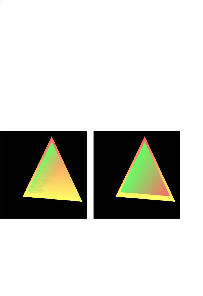
ptg11539634

Correctly Handling Foreground and Background Objects 273

137 return n;

138 }

If you run DepthBuffer , you can see that hidden face removal is performed and that

objects placed at the back are hidden by objects located at the front. This demonstrates

that the hidden surface removal function can eliminate the hidden surfaces regardless of

the position of the eye point. Equally, this also shows that in anything but a trivial 3D

scene, you will always need to enable hidden surface removal and systematically clear the

depth buffer before any drawing operation.

You should note that hidden surface removal requires you to correctly set up the viewing

volume. If you fail to do this (use WebGL in its default configuration), you are likely

to see incorrect results. You can specify either a box or a quadrangular pyramid for the

viewing volume.

Z Fighting

Hidden surface removal is a sophisticated and powerful feature of WebGL that correctly

handles most of the cases where surfaces need to be removed. However, it fails when two

geometrical shapes or objects are located at extremely close positions and results in the

display looking a little unnatural. This phenomenon is known as Z fighting and is illus-

trated in Figure 7.30 . Here, we draw two triangles sharing the same z coordinate.

Figure 7.30 Visual artifact generated by Z fighting (the left side)

The Z fighting occurs because of the limited precision of the depth buffer and means the

system is unable to asses which object is in front and which is behind. Technically, when

handling 3D models, you could avoid this by paying thorough attention to the z coordi-

nates’ values at the model creation stage; however, implementing this workaround would

prove to be unrealistic when dealing with the animation of several objects.

ptg11539634

CHAPTER 7 Toward the 3D World

274

To help resolve this problem, WebGL provides a feature known as the polygon offset .

This works by automatically adding an offset to the z coordinate, whose value is a func-

tion of each object’s inclination with respect to the viewer’s line of sight. You only need

to add two lines of code to enable this function.

1. Enabling the polygon offset function:

gl.enable(gl.POLYGON_OFFSET_FILL);

2. Specifying the parameter used to calculate the offset (before drawing):

gl.polygonOffset(1.0, 1.0);

The same method that enabled the hidden surface removal function is used, but with a

different parameter. The details for

gl.polygonOffset() are shown here.

gl.polygonOffset(factor, units)

Specify the offset to be added to the z coordinate of each vertex drawn afterward.

The offset is calculated with the formula m * factor + r * units , where m represents the

inclination of the triangle with respect to the line of sight, and where r is the smallest

difference between two z coordinates values the hardware can distinguish.

Return value None

Errors None

Let’s look at the program

Zfighting , which uses the polygon offset to reduce z fighting

(see Listing 7.11 ).

Listing 7.11 Zfighting.js

1 // Zfighting.js

…

23 function main() {

…

69 // Enable the polygon offset function

70 gl.enable(gl.POLYGON_OFFSET_FILL);

71 // Draw a rectangle

72 gl.drawArrays(gl.TRIANGLES, 0, n/2); // The green triangle

73 gl.polygonOffset(1.0, 1.0); // Set the polygon offset

74 gl.drawArrays(gl.TRIANGLES, n/2, n/2); // The yellow triangle

75 }

77 function initVertexBuffers(gl) {

ptg11539634

Hello Cube 275

78 var verticesColors = new Float32Array([

79 // Vertex coordinates and color

80 0.0, 2.5, -5.0 , 0.0, 1.0, 0.0, // The green triangle

81 -2.5, -2.5, -5.0 , 0.0, 1.0, 0.0,

82 2.5, -2.5, -5.0 , 1.0, 0.0, 0.0,

84 0.0, 3.0, -5.0 , 1.0, 0.0, 0.0, // The yellow triangle

85 -3.0, -3.0, -5.0 , 1.0, 1.0, 0.0,

86 3.0, -3.0, -5.0 , 1.0, 1.0, 0.0,

87 ]);

88 var n = 6;

If you look at the program from line 80, you can see that the z coordinate for each vertex

is set to –5.0, so z fighting should occur.

Within the rest of the code, the polygon offset function is enabled at line 70. After

that, the green and yellow triangles are drawn at lines 72 and 74. For ease of reading,

the program uses only one buffer object, so

gl.drawArrays() requires the second and

third arguments to be correctly set. The second argument represents the number of the

vertex to start from, while the third argument gives the number of vertices to be drawn.

Once the green triangle has been drawn, the polygon offset parameter is set using

gl.

polygonOffset() . Subsequently, all the vertices drawn will have their z coordinate offset.

If you load this program, you will see the two triangles drawn correctly with no z fight-

ing effects, as in Figure 7.28 (right side). If you now comment out line 73 and reload the

program, you will notice that z fighting occurs and looks similar to the left side of Figure

7.28 .

Hello Cube

So far, the explanation of various WebGL features has been illustrated using simple trian-

gles. You now have enough understanding of the basics to draw 3D objects. Let’s start by

drawing the cube shown in Figure 7.31 . (The coordinates for each vertex are shown on the

right side.) The program used is called

HelloCube , in which the eight vertices that define

the cube are specified using the following colors: white, magenta (bright reddish-violet),

red, yellow, green, cyan (bright blue), blue, and black. As was explained in Chapter 5 ,

“Using Colors and Texture Images,” because colors between the vertices are interpolated,

the resulting cube is shaded with an attractive color gradient (actually a “color solid,” an

analog of the two-dimensional “color wheel”).

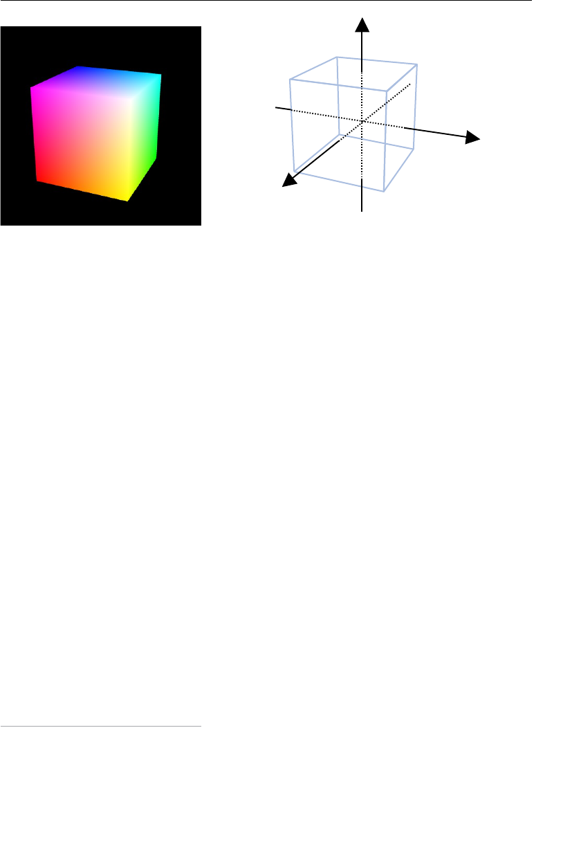
ptg11539634

CHAPTER 7 Toward the 3D World

276

v1(-1,1,1)

v3(1,-1,1)

v4(1,-1,-1)

v0(1,1,1)

v5(1,1,-1)

v2(-1,-1,1)

v7(-1,-1,-1)

v6(-1,1,-1)

white

red

yellow

green

cyan

blue

black

magenta

Figure 7.31 HelloCube and its vertex coordinates

Let’s consider the case where you would like to draw the cube like this with the command

you’ve been relying upon until now: gl.drawArrays() . In this case, you need to draw

using one of the following modes:

gl.TRIANGLES , gl.TRIANGLE_STRIP , or gl.TRIANGLE_FAN .

The most simple and straightforward method would consist of drawing each face with

two triangles. In other words, you can draw a face defined by four vertices (v0, v1, v2, v3),

using two triangles defined by the two sets of three vertices (v0, v1, v2) and (v0, v2, v3),

respectively, and repeat the same process for all the other faces. In this case, the vertices

coordinates specified inside the buffer object would be these:

var vertices = new Float32Array([

1.0, 1.0, 1.0, -1.0, 1.0, 1.0, -1.0, -1.0, 1.0, // v0, v1, v2

1.0, 1.0, 1.0, -1.0, -1.0, 1.0, 1.0, -1.0, 1.0, // v0, v2, v3

1.0, 1.0, 1.0, 1.0, -1.0, 1.0, 1.0, -1.0, -1.0, // v0, v3, v4

…

]);

Because one face is made up of two triangles, you need to know the coordinates of six

vertices to define it. There are six faces, so a total of 6×6 = 36 vertices are necessary. After

having specified the coordinates of each of the 36 vertices, write them in the buffer

object and then call

gl.drawArrays(gl.TRIANGLES, 0, 36), which draws the cube. This

approach requires that you specify and handle 36 vertices, although the cube actually only

requires 8 unique vertices because several triangles share common vertices.

You could, however, take a more frugal approach by drawing a single face with

gl.

TRIANGLE_FAN . Because gl.TRIANGLE_FAN allows you to draw a face defined by the 4-vertex

set (v0, v1, v2, v3), you end up only having to deal with a total of 4×6=24 vertices

4 .

However, you now need to call

gl.drawArrays() separately for each face (six faces). So,

each of these two approaches has both advantages and drawbacks, but neither seems ideal.

4 You can cut down on the number of vertices using this kind of representation. It decreases the

number of necessary vertices to 14, which can be drawn with gl.TRIANGLE_STRIP .

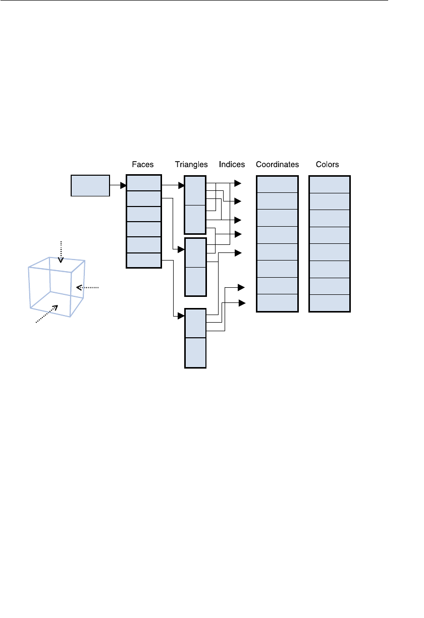
ptg11539634

Hello Cube 277

As you would expect, WebGL has a solution: gl.drawElements() . It’s an alternative way to

directly draw a three-dimensional object in WebGL, with a minimum of vertices. To use

this method, you will need the vertex coordinates of the entire object, which you will use

to explicitly describe how you want WebGL to draw the shape (the cube).

If we break our cube (see the right side of Figure 7.31 ) into vertices that constitute trian-

gles, we get the structure shown in Figure 7.32 . Looking at the left side of the figure,

you can see that Cube points to a Faces list, which, as the name implies, shows that the

cube is split into six faces: front, right, left, top, bottom, and back. In turn, each face is

composed of two triangles picked up from the Triangles list. The numbers in the Triangles

list represent the indices assigned to the Coordinate list. The vertex coordinates’ indices

are numbered in order starting from zero.

thgir

tnorf

cube 1, 1, 1

-1, 1, 1

-1, -1, 1

1, -1, 1

1, -1, -1

1, 1, -1

-1, 1, -1

-1, -1, -1

1, 1, 1

1, 0, 1

1, 0, 0

1, 1, 0

0, 1, 0

0, 1, 1

0, 0, 1

0, 0, 0

v1(-1,1,1)

v3(1,-1,1)

v4(1,-1,-1)

v0(1,1,1)

v5(1,1,-1)

v2(-1,-1,1)

v7(-1,-1,-1)

front

back

down

left

right

v6(-1,1,-1)

Figure 7.32 The associations of the faces that make up the cube, triangles, vertex

coordinates, and colors

This approach results in a data structure that describes the way the object (a cube) can be

built from its vertex and color data.

Drawing the Object with Indices and Vertices Coordinates

So far, you have been using gl.drawArrays() to draw vertices. However, WebGL supports

an alternative approach,

gl.drawElements() , that looks similar to that of gl.draw

Arrays() . However, it has some advantages that we’ll explain later. First, let’s look at

how to use

gl.drawElements() . You need to specify the indices based, not on gl.ARRAY_

BUFFER , but on gl.ELEMENT_ARRAY_BUFFER (introduced in the explanation of the buffer

object in Chapter 4 ). The key difference is that

gl.ELEMENT_ARRAY_BUFFER handles data

structured by the indices.

ptg11539634

CHAPTER 7 Toward the 3D World

278

gl.drawElements(mode, count, type, offset)

Executes the shader and draws the geometric shape in the specified mode using the

indices specified in the buffer object bound to

gl.ELEMENT_ARRAY_BUFFER .

Parameters mode Specifies the type of shape to be drawn (refer to Figure

3.17 ).

The following symbolic constants are accepted:

gl.POINTS, gl.LINE_STRIP, gl.LINE_LOOP, gl.LINES,

gl.TRIANGLE_STRIP, gl.TRIANGLE_FAN , or gl.TRIANGLES

count Number of indices to be drawn (integer).

type Specifies the index data type:

gl.UNSIGNED_BYTE or gl.

UNSIGNED_SHORT

offset Specifies the offset in bytes in the index array where you

want to start rendering.

Return value None

Errors INVALID_ENUM mode is none of the preceding values.

INVALID_VALUE A negative value is specified for count or offset

Writing indices to the buffer object bound to

gl.ELEMENT_ARRAY_BUFFER is done in the

same way you write the vertex information to the buffer object with

gl.drawArrays() .

That is to say, you use

gl.bindBuffer() and gl.bufferData() , but the only difference is

that the first argument,

target , is set to gl.ELEMENT_ARRAY_BUFFER . Let’s take a look at the

sample program.

Sample Program (HelloCube.js)

The sample program is shown in Listing 7.12 . The vertex and fragment shaders set a quad-

rangular pyramid viewing volume and perform a perspective projection transformation

ProjectiveView_mvpMatrix.js . It’s important to understand that gl.drawElements()

doesn’t do anything special. The vertex shader simply transforms the vertex coordinates,

and the fragment shader sets the color passed by the varying variable to

gl_FragColor .

The key difference from the previous programs comes down to the processing of the

buffer object in

initVertexBuffers() .

5 Even if type doesn’t correspond to the type ( Uint8Array or Uint16Array ) of the data array speci ed

in gl.ELEMENT_ARRAY_BUFFER , no error is returned. However, if, for example, you specify the index

with a Uint16Array type, and set type to gl.UNSIGNED_BYTE , in some cases, the object might not

be completely displayed.

ptg11539634

Hello Cube 279

Listing 7.12 HelloCube.js

1 // HelloCube.js

2 // Vertex shader program

3 var VSHADER_SOURCE =

…

8 ‘void main() {n’ +

9 ‘ gl_Position = u_MvpMatrix * a_Position;n’ +

10 ‘ v_Color = a_Color;n’ +

11 ‘}n’;

13 // Fragment shader program

14 var FSHADER_SOURCE =

…

19 ‘void main() {n’ +

20 ‘ gl_FragColor = v_Color;n’ +

21 ‘}n’;

23 function main() {

…

40 // Set the vertex coordinates and color

41 var n = initVertexBuffers(gl);

…

47 // Set the clear color and enable the hidden surface removal

48 gl.clearColor(0.0, 0.0, 0.0, 1.0);

49 gl.enable(gl.DEPTH_TEST);

…

58 // Set the eye point and the viewing volume

59 var mvpMatrix = new Matrix4();

60 mvpMatrix.setPerspective(30, 1, 1, 100);

61 mvpMatrix.lookAt(3, 3, 7, 0, 0, 0, 0, 1, 0);

63 // Pass the model view projection matrix to u_MvpMatrix

64 gl.uniformMatrix4fv(u_MvpMatrix, false, mvpMatrix.elements);

66 // Clear the color and depth buffer

67 gl.clear(gl.COLOR_BUFFER_BIT | gl.DEPTH_BUFFER_BIT);

69 // Draw the cube

70 gl.drawElements(gl.TRIANGLES, n, gl.UNSIGNED_BYTE, 0);

71 }

73 function initVertexBuffers(gl) {

…

82 var verticesColors = new Float32Array([

ptg11539634

CHAPTER 7 Toward the 3D World

280

83 // Vertex coordinates and color

84 1.0, 1.0, 1.0, 1.0, 1.0, 1.0, // v0 White

85 -1.0, 1.0, 1.0, 1.0, 0.0, 1.0, // v1 Magenta

86 -1.0, -1.0, 1.0, 1.0, 0.0, 0.0, // v2 Red

…

91 -1.0, -1.0, -1.0, 0.0, 0.0, 0.0 // v7 Black

92 ]);

94 // Indices of the vertices

95 var indices = new Uint8Array([

96 0, 1, 2, 0, 2, 3, // front

97 0, 3, 4, 0, 4, 5, // right

98 0, 5, 6, 0, 6, 1, // up

99 1, 6, 7, 1, 7, 2, // left

100 7, 4, 3, 7, 3, 2, // down

101 4, 7, 6, 4, 6, 5 // back

102 ]);

103

104 // Create a buffer object

105 var vertexColorBuffer = gl.createBuffer();

106 var indexBuffer = gl.createBuffer();

…

111 // Write the vertex coordinates and color to the buffer object

112 gl.bindBuffer(gl.ARRAY_BUFFER, vertexColorBuffer);

113 gl.bufferData(gl.ARRAY_BUFFER, verticesColors, gl.STATIC_DRAW);

114

115 var FSIZE = verticesColors.BYTES_PER_ELEMENT;

116 // Assign the buffer object to a_Position and enable it

117 var a_Position = gl.getAttribLocation(gl.program, ‘a_Position’);

…

122 gl.vertexAttribPointer(a_Position, 3, gl.FLOAT, false, FSIZE * 6, 0);

123 gl.enableVertexAttribArray(a_Position);

124 // Assign the buffer object to a_Position and enable it

125 var a_Color = gl.getAttribLocation(gl.program, ‘a_Color’);

…

130 gl.vertexAttribPointer(a_Color, 3, gl.FLOAT, false, FSIZE * 6, FSIZE * 3);

131 gl.enableVertexAttribArray(a_Color);

132

133 // Write the indices to the buffer object

134 gl.bindBuffer(gl.ELEMENT_ARRAY_BUFFER, indexBuffer);

135 gl.bufferData(gl.ELEMENT_ARRAY_BUFFER, indices, gl.STATIC_DRAW);

136

137 return indices.length;

138 }

ptg11539634

Hello Cube 281

The processing flow in the JavaScript main() is the same as in ProjectiveView_mvpMatrix.

js , but let’s quickly review it. After having written the vertex data in the buffer object

through a call to

initVertexBuffers() at line 41, you enable the hidden surface removal

function at line 49. This is necessary to allow WebGL to correctly draw the cube, taking

into consideration the relationship between the front and the back faces.

You set the eye point and the viewing volume from line 59 to line 61 and pass the model

view projection matrix to the vertex shader’s uniform variable

u_MvpMatrix .

At line 67, you clear the color and depth buffers and then draw the cube using

gl.drawElements() at line 70. The use of gl.drawElements() in this program is the

main difference to

ProjectiveView_mvpMatrix.js , so let’s take a look at that.

Writing Vertex Coordinates, Colors, and Indices to the Buffer Object

The method to assign the vertex coordinates and the color information to the attribute

variable using the buffer object in

initVertexBuffers() is unchanged. This time, because

you won’t necessarily use the vertex information in the order specified in the object

buffer, you need to additionally specify in which order you will use it. For that you will

use the vertex order specified in

verticesColors as indices. In short, the vertex informa-

tion specified first in the buffer object will be set to index 0, the vertex information speci-

fied in second place in the buffer object will be set to index 1, and so on. Here, we show

the part of the program that specifies the indices in

initVertexBuffers() :

73 function initVertexBuffers(gl) {

…

82 var verticesColors = new Float32Array([

83 // Vertex coordinates and color

84 1.0, 1.0, 1.0, 1.0, 1.0, 1.0, // v0 White

85 -1.0, 1.0, 1.0, 1.0, 0.0, 1.0, // v1 Magenta

…

91 -1.0, -1.0, -1.0, 0.0, 0.0, 0.0 // v7 Black

92 ]);

94 // Indices of the vertex coordinates

95 var indices = new Uint8Array([

96 0, 1, 2, 0, 2, 3, // front

97 0, 3, 4, 0, 4, 5, // right

98 0, 5, 6, 0, 6, 1, // up

99 1, 6, 7, 1, 7, 2, // left

100 7, 4, 3, 7, 3, 2, // down

101 4, 7, 6, 4, 6, 5 // back

102 ]);

103

104 // Create a buffer object

105 var vertexColorBuffer = gl.createBuffer();

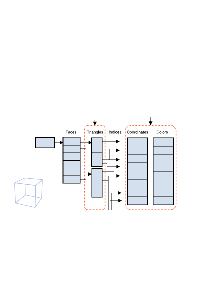
ptg11539634

CHAPTER 7 Toward the 3D World

282

106 var indexBuffer = gl.createBuffer();

…

136 // Write the indices to the buffer object

137 gl.bindBuffer(gl.ELEMENT_ARRAY_BUFFER, indexBuffer);

138 gl.bufferData(gl.ELEMENT_ARRAY_BUFFER, indices, gl.STATIC_DRAW);

139

140 return indices.length;

141 }

As you may have noticed, at line 106, you create the buffer object ( indexBuffer ) in which

to write the indices. These indices are stored in the array

indices at line 95. Because the

indices are integers (0, 1, 2, …), you use an integer typed array

Uint8Array (unsigned

8-bit encoded integer). If there are more than 256 indices, use

Uint16Array instead. The

content of this array is the triangles list of Figure 7.33 , where each grouping of three

indices points to the three vertex coordinates for that triangle. Generally, this index

doesn’t need to be manually created because 3D modeling tools, introduced in the next

chapter, usually generate it along with the vertices information.

cube 1, 1, 1

-1, 1, 1

-1, -1, 1

1, -1, 1

1, -1, -1

1, 1, -1

-1, 1, -1

-1, -1, -1

1, 1, 1

1, 0, 1

1, 0, 0

1, 1, 0

0, 1, 0

0, 1, 1

0, 0, 1

0, 0, 0

gl.ELEMENT_ARRAY_BUFFER gl.ARRAY_BUFFER

v6(-1,1,-1)

v1(-1,1,1)

v3(1,-1,1)

v4(1,-1,-1)

v0(1,1,1)

v5(1,1,-1)

v2(-1,-1,1)

v7(-1,-1,-1)

front

back

down

left

right

Figure 7.33 Contents of gl.ELEMENT_ARRAY_BUFFER and gl.ARRAY_BUFFER

The setup for the specified indices is performed at lines 134 and 135. This is similar to the

way buffer objects have been written previously, with the difference that the first argu-

ment is modified to

gl.ELEMENT_ARRAY_BUFFER . This is to let the WebGL system know that

the contents of the buffer are indices.

Once executed, the internal state of the WebGL system is as detailed in Figure 7.34 .

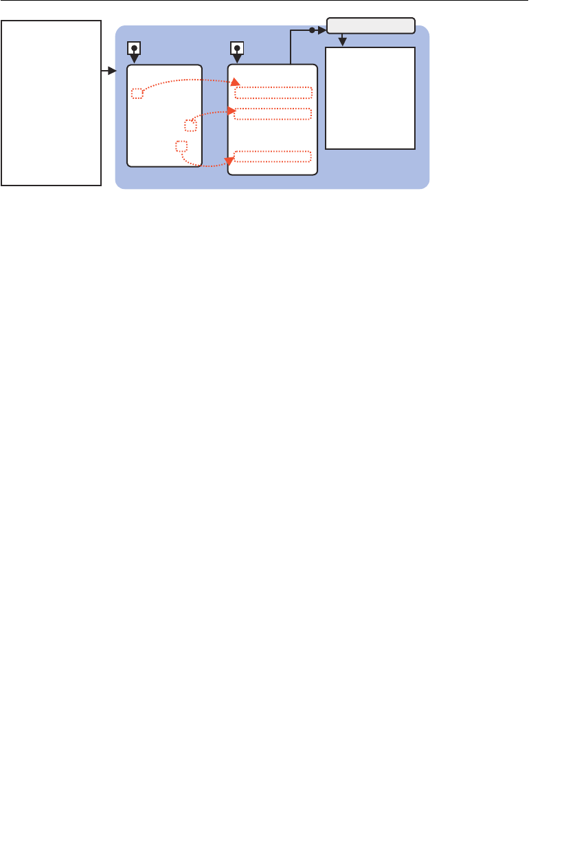
ptg11539634

Hello Cube 283

tnemgarF

redahS

tpircSavaJ

{)(niamnoitcnuf

…LGbeWteg=lgrav

…

;)…(reffuBdnib.lg

REFFUB_YARRA_TNEM

ELE.lg

tcejbOreffuB

,3,2,0,2,1,0

,5,4,0,4,3,0

,1,6,0,6,5,0

,2,7,1,7,6,1

,2,3,7,3,4,7

5,6,4,6,7,4

tcejbOreffuB

,1,1,1,1,1,1

,1,0,1,1,1,1—

,0,0,1,1,1—,1—

,0,1,1,1,1—,1

,0,1,0,1—,1—,1

,1,1,0,1—,1,1

,,,,—,, 100111—

0,0,0,1—,1—,1 —

REFFUB_YARRA.lg

elbairavetubirtta

Figure 7.34 gl.ELEMENT_ARRAY_BUFFER and gl.ARRAY_BUFFER

Once set up, the call to

gl.drawElements() at line 70 draws the cube:

69 // Draw the cube

70 gl.drawElements(gl.TRIANGLES, n, gl.UNSIGNED_BYTE, 0);

You should note that the second argument of gl.drawElements() , the number of indices,

represents the number of vertex coordinates involved in the drawing, but it is not identi-

cal to the number of vertices coordinates written to

gl.ARRAY_BUFFER .

When you call gl.drawElements() , the indices are extracted from the buffer object

(

indexBuffer ) bound to gl.ELEMENT_ARRAY_BUFFER , while the associated vertex informa-

tion is retrieved from the buffer object (

vertexColorBuffer ) bound to gl.ARRAY_BUFFER .

All these pieces of information are then passed to the attribute variable. The process is

repeated for each index, and then the whole cube gets drawn by a single call to

gl.drawElements() . With this approach, because you refer to the vertex information

through indices, you can recycle the vertex information. Although

gl.drawElements()

allows you to curb memory usage by sharing the vertex information, the cost is a process

to convert the indices to vertex information (that is, a level of indirection). This means

that the choice between

gl.drawElements() and gl.drawArrays() , because they both

have pros and cons, will eventually depend on the system implementation.

At this stage, although it’s clear that

gl.drawElements() is an efficient way to draw 3D

shapes, one key feature is missing. There is no way to control color, so it is helpful to draw

a cube using a single solid color, as shown in Figure 7.31 .

For example, let’s consider the case where you would like to modify the color of each face

of the cube, as shown in Figure 7.35 , or map textures to the faces. You need to know the

color or texture information for each face, yet you cannot implement this with the combi-

nation of indices, triangle list, and vertex coordinates shown in Figure 7.33 .

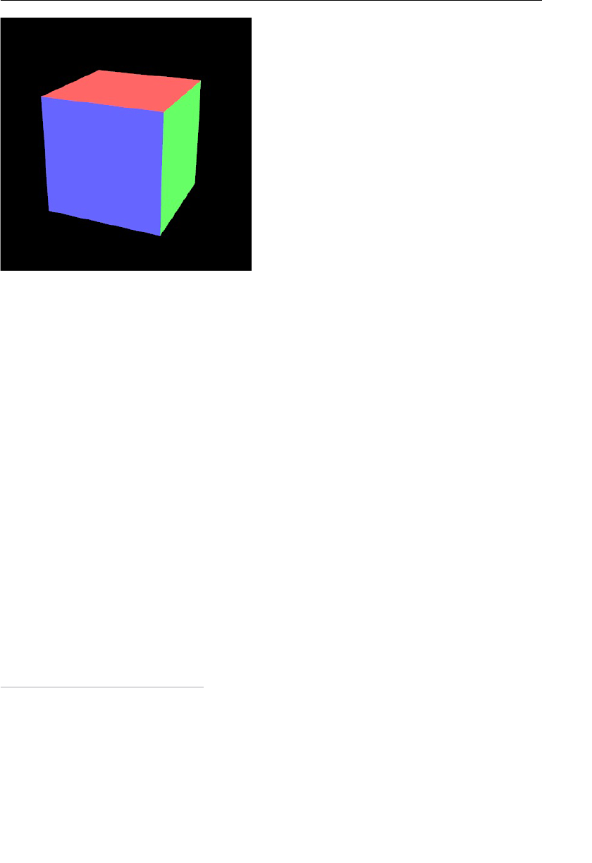
ptg11539634

CHAPTER 7 Toward the 3D World

284

Figure 7.35 Cube with differently colored faces

In the following section, we will examine how to address this problem and specify the

color information for each face.

Adding Color to Each Face of a Cube

As discussed before, you can only pass per-vertex information to the vertex shader. This

implies that you need to pass the face’s color and the vertices of the triangles as vertex

information to the vertex shader. For instance, to draw the “front” face in blue, made up

of v0, v1, v2, and v3 ( Figure 7.33 ), you need to specify the same blue color for each of the

vertices.

However, as you may have noticed, v0 is also shared by the “right” and “top” faces as well

as the “front” face. Therefore, if you specify the color blue for the vertices that form the

“front” face, you are then unable to choose a different color for those vertices that also

belong to another face. To cope with this problem, although this might not seem as effi-

cient, you must create duplicate entries for the shared vertices in the vertices coordinates

listing, as illustrated in Figure 7.36 . Doing so, you will have to handle common vertices

with identical coordinates in the face’s triangle list as separate entities.

6 If you break down all the faces into triangles and draw using gl.drawArrays() , you have

to process 6 vertices * 6 faces = 36 vertices, so the difference between gl.drawArrays() and

gl.drawElements() in memory usage is negligible. This is because a cube or a cuboid is a special

3D object whose faces are connected vertically; therefore, each vertex needs to have three colors.

However, in the case of complex 3D models, specifying several colors to a single vertex would be rare.

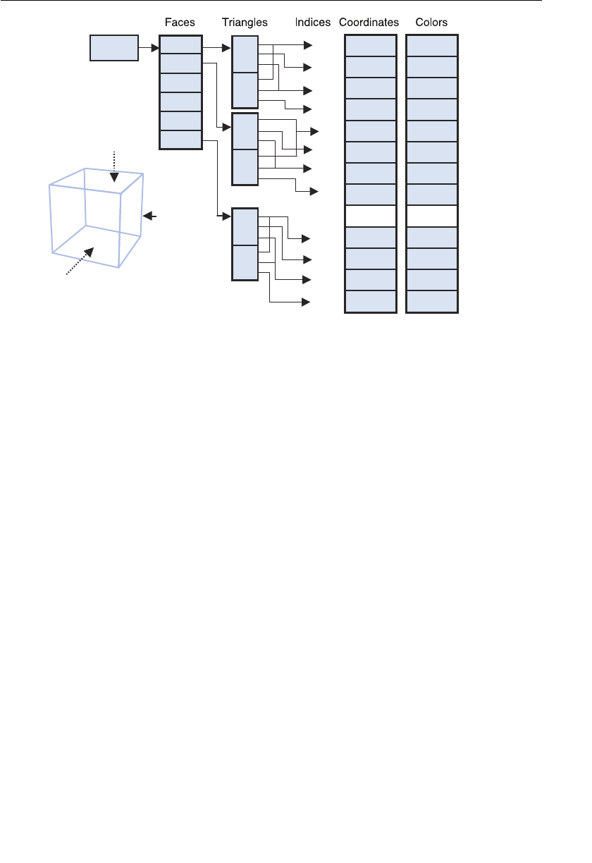
ptg11539634

Hello Cube 285

ebuc 0z,0y,0x

1z,1y,1x

2z,2y,2x

3z,3y,3x

0z,0y,0x

3z,3y,3x

4z,4y,4x

5z,5y,5x

4z,4y,4x

7z,7y,7x

6z,6y,6x

5z,5y,5x

1,0,0

0,1,0

1,1,0

……

)eulb(tnorf

)der(pu

)neerg(thgir

back

down

left

right

front 0

v6(-1,1,-1)

v1(-1,1,1)

v3(1,-1,1)

v4(1,-1,-1)

v0(1,1,1)

v5(1,1,-1)

v2(-1,-1,1)

v7(-1,-1,-1)

Figure 7.36 The faces that constitute the cube, the triangles, and the relationship between

vertices coordinates (configured so that you can choose a different color for each face)

When opting for such a configuration, the contents of the index list, which consists of

the face’s triangle list, will differ from face to face, thus allowing you to modify the color

for each face. This approach can also be used if you want to map a texture to each face.

You would need to specify the texture coordinates for each vertex, but you can actually

deal with this by rewriting the color list ( Figure 7.36 ) as texture coordinates. The sample

program in the section “Rotate Object” in Chapter 10 covers this approach in more detail.

Let’s take a look at the sample program

ColoredCube , which displays a cube with each face

painted a different color. The screen shot of

ColoredCube is identical to Figure 7.35 .

Sample Program (ColoredCube.js)

The sample program is shown in Listing 7.13 . Because the only difference from

HelloCube.js is the method of storing vertex information into the buffer object, let’s look

in more detail at the code related to the

initVertexBuffers() . The main differences to

HelloCube.js are

• In HelloCube.js , the vertex coordinates and color are stored in a single buffer

object, but because this make the array unwieldy, the program has been modified so

that they are now stored in separate buffer objects.

• The respective contents of the vertex array (which stores the vertex coordinates), the

color array (which stores the color information), and the index array (which stores

the indices) are modified in accordance with the configuration described in Figure

7.36 (lines 83, 92, and 101).

ptg11539634

CHAPTER 7 Toward the 3D World

286

• To keep the sample program as compact as possible, the function

initArrayBuffer() is defined, which bundles the buffer object creation, binding,

writing of data, and enabling (lines 116, 119, and 129).

As you examine the program, take note of how the second bullet is implemented to match

the structure shown in Figure 7.36 .

Listing 7.13 ColoredCube.js

1 // ColoredCube.js

…

23 function main() {

…

40 // Set the vertex information

41 var n = initVertexBuffers(gl);

…

69 // Draw the cube

70 gl.drawElements(gl.TRIANGLES, n, gl.UNSIGNED_BYTE, 0);

71 }

73 function initVertexBuffers(gl) {

…

83 var vertices = new Float32Array([ // Vertex coordinates

84 1.0, 1.0, 1.0, -1.0, 1.0, 1.0, -1.0,-1.0, 1.0, 1.0,-1.0, 1.0,

85 1.0, 1.0, 1.0, 1.0,-1.0, 1.0, 1.0,-1.0,-1.0, 1.0, 1.0,-1.0,

86 1.0, 1.0, 1.0, 1.0, 1.0,-1.0, -1.0, 1.0,-1.0, -1.0, 1.0, 1.0,

…

89 1.0,-1.0,-1.0, -1.0,-1.0,-1.0, -1.0, 1.0,-1.0, 1.0, 1.0,-1.0

90 ]);

92 var colors = new Float32Array([ // Colors

93 0.4, 0.4, 1.0, 0.4, 0.4, 1.0, 0.4, 0.4, 1.0, 0.4, 0.4, 1.0,

94 0.4, 1.0, 0.4, 0.4, 1.0, 0.4, 0.4, 1.0, 0.4, 0.4, 1.0, 0.4,

95 1.0, 0.4, 0.4, 1.0, 0.4, 0.4, 1.0, 0.4, 0.4, 1.0, 0.4, 0.4,

…

98 0.4, 1.0, 1.0, 0.4, 1.0, 1.0, 0.4, 1.0, 1.0, 0.4, 1.0, 1.0

99 ]);

100

101 var indices = new Uint8Array([ // Indices of the vertices

102 0, 1, 2, 0, 2, 3, // front

103 4, 5, 6, 4, 6, 7, // right

104 8, 9,10, 8,10,11, // up

…

107 20,21,22, 20,22,23 // back

108 ]);

ptg11539634

Hello Cube 287

109

110 // Create a buffer object

111 var indexBuffer = gl.createBuffer();

…

115 // Write the vertex coordinates and color to the buffer object

116 if (!initArrayBuffer(gl, vertices, 3, gl.FLOAT, ‘a_Position’))

117 return -1;

118

119 if (!initArrayBuffer(gl, colors, 3, gl.FLOAT, ‘a_Color’))

120 return -1;

…

122 // Write the indices to the buffer object

123 gl.bindBuffer(gl.ELEMENT_ARRAY_BUFFER, indexBuffer);

124 gl.bufferData(gl.ELEMENT_ARRAY_BUFFER, indices, gl.STATIC_DRAW);

125

126 return indices.length;

127 }

128

129 function initArrayBuffer(gl, data, num, type, attribute) {

130 var buffer = gl.createBuffer(); // Create a buffer object

…

135 // Write date into the buffer object

136 gl.bindBuffer(gl.ARRAY_BUFFER, buffer);

137 gl.bufferData(gl.ARRAY_BUFFER, data, gl.STATIC_DRAW);

138 // Assign the buffer object to the attribute variable

139 var a_attribute = gl.getAttribLocation (gl.program, attribute);

…

144 gl.vertexAttribPointer(a_attribute, num, type, false, 0, 0);

145 // Enable the assignment of the buffer object to the attribute variable

146 gl.enableVertexAttribArray(a_attribute);

147

148 return true;

149 }

Experimenting with the Sample Program

In ColoredCube , you specify a different color for each face. So what happens when you

choose an identical color for all the faces? For example, let’s try to set the color infor-

mation in

ColoredCube.js ’s colors array to “white,” as shown next. We will call this

program

ColoredCube_singleColor.js :

1 // ColoredCube_singleColor.js

…

92 var colors = new Float32Array([

93 1.0, 1.0, 1.0, 1.0, 1.0, 1.0, 1.0, 1.0, 1.0, 1.0, 1.0, 1.0,

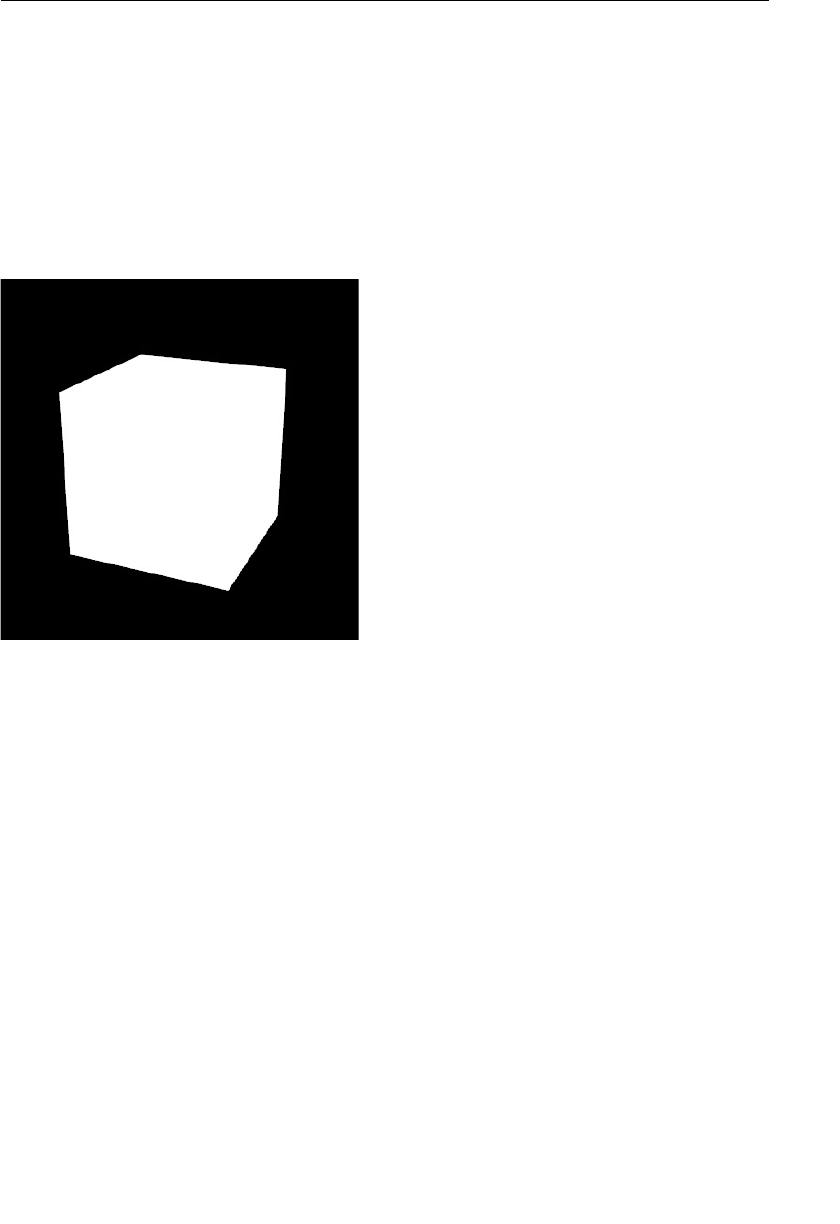
ptg11539634

CHAPTER 7 Toward the 3D World

288

94 1.0, 1.0, 1.0, 1.0, 1.0, 1.0, 1.0, 1.0, 1.0, 1.0, 1.0, 1.0,

…

98 1.0, 1.0, 1.0, 1.0, 1.0, 1.0, 1.0, 1.0, 1.0, 1.0, 1.0, 1

99 ]);

When you execute the program, you see an output like the screenshot shown in Figure

7.37 . One result of using a single color is that it becomes difficult to actually recognize

the cube. Up until now you could differentiate each face because they were differently

colored; therefore, you could recognize the whole shape as a solid. However, when you

switch to a unique color, you lose this three-dimensional impression.

Figure 7.37 Cube with its faces being identically colored

In contrast, in the real world, when you put a white box on a table, you can identify it as

a solid (see Figure 7.38 ). This is because each face, although the same white color, presents

a slightly different appearance because each is lit slightly differently. In

ColoredCube_

singleColor , such an effect is not programmed, so the cube is hard to recognize. We will

explore how to correctly light 3D scenes in the next chapter.

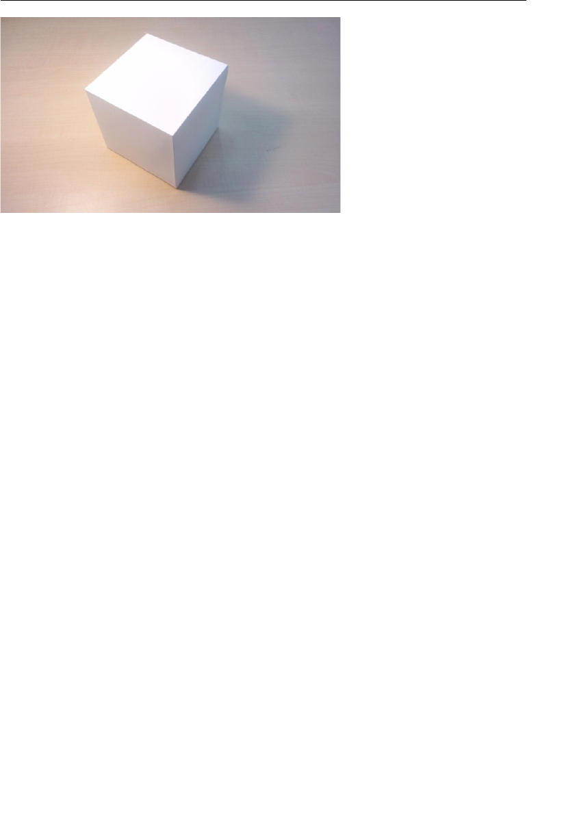
ptg11539634

Hello Cube 289

Figure 7.38 White box in the real world

Summary

In this chapter, through the introduction of the depth information, you have examined

setting the viewer’s eye point and viewing volume, looked at how to draw real 3D objects,

and briefly examined the local and world coordinate system. Many of the examples were

similar to those previously explained for the two-dimensional world, except for the intro-

duction of the z-axis to handle depth information.

The next chapter explains how to light 3D scenes and how to draw and manipulate

three-dimensional shapes with complex structures. We will also return to the function

initShaders() , which has hidden a number of complex issues that you now have enough

understanding to explore.

ptg11539634

This page intentionally left blank

ptg11539634

Chapter 8

Lighting Objects

This chapter focuses on lighting objects, looking at different light sources and

their effects on the 3D scene. Lighting is essential if you want to create realistic

3D scenes because it helps to give the scene a sense of depth.

The following key points are discussed in this chapter:

• Shading, shadows, and different types of light sources including point,

directional, and ambient

• Reflection of light in the 3D scene and the two main types: diffuse and

ambient

• The details of shading and how to implement the effect of light to make

objects, such as the pure white cube in the previous chapter, look three-

dimensional

By the end of this chapter, you will have all the knowledge you need to create

lighted 3D scenes populated with both simple and complex 3D objects.

Lighting 3D Objects

When light hits an object in the real world, part of the light is reflected by the

surface of the object. Only after this reflected light enters your eyes can you see

the object and distinguish its color. For example, a white box reflects white light

which, when it enters your eyes, allows you to tell that the box is white.

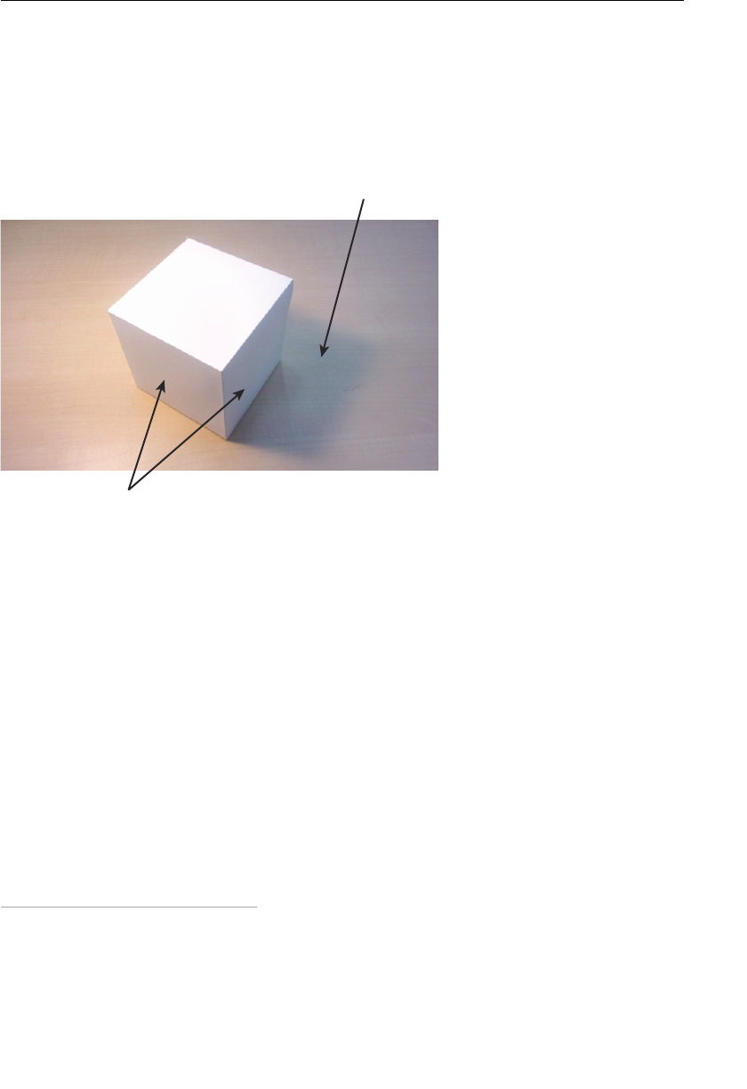
ptg11539634

CHAPTER 8 Lighting Objects

292

In the real world, two important phenomena occur when light hits an object

(see Figure 8.1 ):

• Depending on the light source and direction, surface color is shaded.

• Depending on the light source and direction, objects “cast” shadows on the ground

or the floor.

Shadowing

Shading

Figure 8.1 Shading and shadowing

In the real world, you usually notice shadows, but you quite often don’t notice shading,

which gives 3D objects their feeling of depth. Shading is subtle but always present. As

shown in Figure 8.1 , even surfaces of a pure white cube are distinguishable because each

surface is shaded differently by light. As you can see, the surfaces hit by more light are

brighter, and the surfaces hit by less light are darker, or more shaded. These differences

allow you to distinguish each surface and ensure that the cube looks cubic.

In 3D graphics, the term shading

1 is used to describe the process that re-creates this

phenomenon where the colors differ from surface to surface due to light. The other

phenomenon, that the shadow of an object falls on the floor or ground, is re-created using

a process called shadowing . This section discusses shading. Shadowing is discussed in

Chapter 10 , which focuses on a set of useful techniques that build on your basic knowl-

edge of WebGL.

1 Shading is so critical to 3D graphics that the core language, GLSL ES, is a shader language, the

OpenGL ES Shading Language. The original purpose of shaders was to re-create the phenomena of

shading.

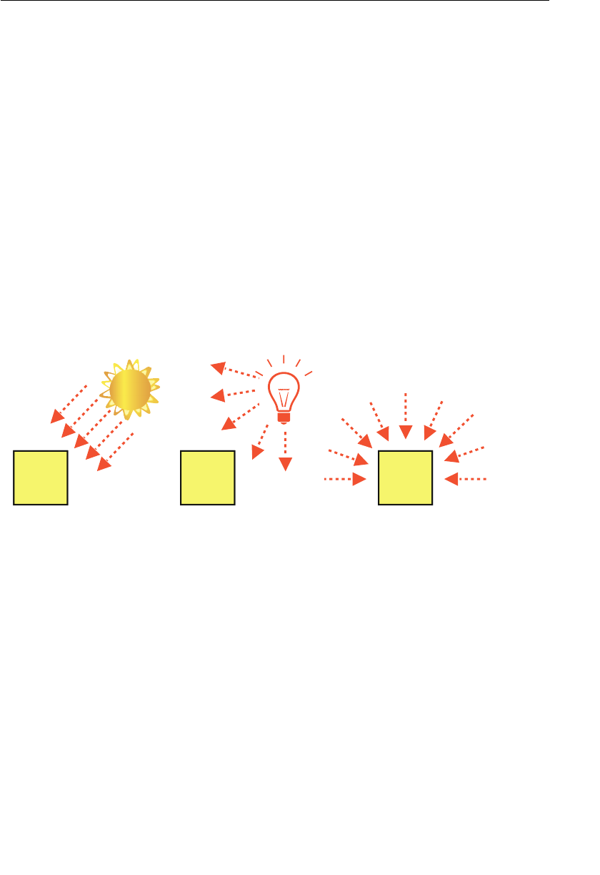
ptg11539634

Lighting 3D Objects 293

When discussing shading, you need to consider two things:

• The type of light source that is emitting light

• How the light is reflected from surfaces of an object and enters the eye

Before we begin to program, let’s look at different types of light sources and how light is

reflected from different surfaces.

Types of Light Source

When light illuminates an object, a light source emits the light. In the real world, light

sources are divided into two main categories: directional light , which is something like

the sun that emits light naturally, and point light , which is something like a light bulb

that emits light artificially. In addition, there is ambient light that represents indirect

light (that is, light emitted from all light sources and reflected by walls or other objects

(see Figure 8.2 ). In 3D graphics, there are additional types of light sources. For example,

there is a spot light representing flashlights, headlamps, and so on. However, in this book,

we don’t address these more specialized light sources. Refer to the book OpenGL ES 2.0

Programming Guide for further information on these specialized light sources.

thgiltneibmAthgiltnioPthgillanoitceriD

Figure 8.2 Directional light, point light, and ambient light

Focusing on the three main types of light source covered in this book:

Directional light: A directional light represents a light source whose light rays are paral-

lel. It is a model of light whose source is considered to be at an infinite distance, such

as the sun. Because of the distance travelled, the rays are effectively parallel by the time

they reach the earth. This light source is considered the simplest, and because its rays are

parallel can be specified using only direction and color.

Point light: A point light represents a light source that emits light in all directions from

one single point. It is a model of light that can be used to represent light bulbs, lamps,

ptg11539634

CHAPTER 8 Lighting Objects

294

flames, and so on. This light source is specified by its position and color.

2 However, the

light direction is determined from the position of the light source and the position at

which the light strikes a surface. As such, its direction can change considerably within

the scene.

Ambient light: Ambient light (indirect light) is a model of light that is emitted from

the other light source (directional or point), reflected by other objects such as walls, and

reaches objects indirectly. It represents light that illuminates an object from all directions

and has the same intensity.

3 For example, if you open the refrigerator door at night, the

entire kitchen becomes slightly lighter. This is the effect of the ambient light. Ambient

light does not have position and direction and is specified only by its color.

Now that you know the types of light sources that illuminate objects, let’s discuss how

light is reflected by the surface of an object and then enters the eye.

Types of Reflected Light

How light is reflected by the surface of an object and thus what color the surface will

become is determined by two things: the type of the light and the type of surface of the

object. Information about the type of light includes its color and direction. Information

about the surface includes its color and orientation.

When calculating reflection from a surface, there are two main types: diffuse reflection

and environment (or ambient ) reflection . The remainder of this section describes how to

calculate the color due to reflection using the two pieces of information described earlier.

There is a little bit of math to be considered, but it’s not complicated.

Diffuse Reflection

Diffuse reflection is the reflection of light from a directional light or a point light. In

diffuse reflection, the light is reflected (scattered) equally in all directions from where

it hits (see Figure 8.3 ). If a surface is perfectly smooth like a mirror, all incoming light

is reflected; however, most surfaces are rough like paper, rock, or plastic. In such cases,

the light is scattered in random directions from the rough surface. Diffuse reflection is a

model of this phenomenon.

2 This type of light actually attenuates; that is, it is strong near the source and becomes weaker farther

from the source. For the sake of simplicity of the description and sample programs, light is treated

as nonattenuating in this book. For attenuation, please refer to the book OpenGL ES 2.0 Programming

Guide .

3 In fact, ambient light is the combination of light emitted from light sources and re ected by various

surfaces. It is approximated in this way because it would otherwise need complicated calculations to

take into account all the many light sources and how and where they are re ected.

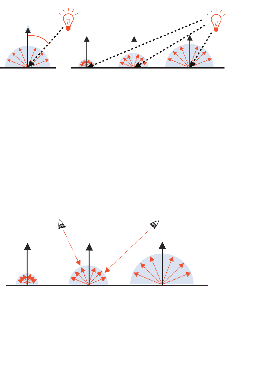
ptg11539634

Lighting 3D Objects 295

orientation of

the surface

AB C

orientation of

the surface

diffuse reflection

light

direction

light

source

light

source

diffuse reflection (reflection differs by light direction)

Figure 8.3 Diffuse reflection

In diffuse reflection, the color of the surface is determined by the color and the direction

of light and the base color and orientation of the surface. The angle between the light

direction and the orientation of the surface is defined by the angle formed by the light

direction and the direction “perpendicular” to the surface. Calling this angle θ , the surface

color by diffuse reflection is calculated using the following formula.

Equation 8.1

〈〉=

〈〉×〈〉×

surface color by diffuse reflection

light color base color of surface

 

cos 

where < light color > is the color of light emitted from a directional light or a point light.

Multiplication with the <base color of the surface> is performed for each RGB component

of the color. Because light by diffuse reflection is scattered equally in all directions from

where it hits, the intensity of the reflected light at a certain position is the same from

any angle (see Figure 8.4 ).

ecafrusehtfonoitatneiro

Figure 8.4 The intensity of light at a given position is the same from any angle

Ambient Reflection

Ambient reflection is the reflection of light from another light source. In ambient reflec-

tion, the light is reflected at the same angle as its incoming angle. Because an ambient

light illuminates an object equally from all directions with the same intensity, its bright-

ness is the same at any position (see Figure 8.5 ). It can be approximated as follows.

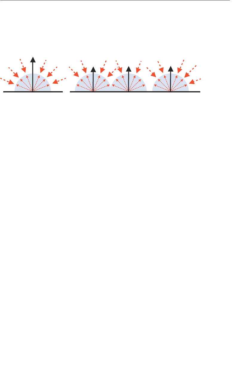
ptg11539634

CHAPTER 8 Lighting Objects

296

Equation 8.2

〈〉=

〈〉×〈〉

surface color by ambient reflection

light color base color of surface

 



where <light color> is the color of light emitted from other light source.

eflectionrtneibma eflectionr eflectionrtneibmaemaseht()noitisopynata

orientation of the surface

Figure 8.5 Ambient reflection

When both diffuse reflection and ambient reflection are present, the color of the surface is

calculated by adding, as follows.

Equation 8.3

〈〉=

〈〉+〈〉

surface color by diffuse and ambient reflection

surface color by diffuse reflection surface color by ambient reflection

  

   

Note that it is not required to always use both light sources, or use the formulas exactly

as mentioned here. You are free to modify each formula to achieve the effect you require

when showing the object.

Now let’s construct some sample programs that perform shading (shading and coloring

the surfaces of an object by placing a light source at an appropriate position). First let’s try

to implement shading due to directional light and its diffuse reflection.

Shading Due to Directional Light and Its Diffuse Reflection

As described in the previous section, surface color is determined by light direction and the

orientation of the surface it strikes when considering diffuse reflection. The calculation of

the color due to directional light is easy because its direction is constant. The formula for

calculating the color of a surface by diffuse reflection ( Equation 8.1 ) is shown again here:

〈〉=

〈〉×〈〉×

surface color by diffuse reflection

light color base color of surface

 

cos 

The following three pieces of information are used:

• The color of the light source (directional light)

• The base color of the surface

• The angle (

) between the light and the surface

ptg11539634

Lighting 3D Objects 297

The color of a light source may be white, such as sunlight, or other colors, such as the

orange of lighting in road tunnels. As you know, it can be represented by RGB. White

light such as sunlight has an RGB value of (1.0, 1.0, 1.0). The base color of a surface

means the color that the surface was originally defined to have, such as red or blue. To

calculate the color of a surface, you need to apply the formula for each of the three RGB

components; the calculation is performed three times.

For example, assume that the light emitted from a light source is white (1.0, 1.0, 1.0), and

the base color of the surface is red (1.0, 0.0, 0.0). From Equation 8.1 , when

is 0.0 (that is,

when the light hits perpendicularly), cos

becomes 1.0. Because the R component of the

light source is 1.0, the R component of the base surface color is 1.0, and the cos

is 1.0,

the R component of the surface color by diffuse reflection is calculated as follows:

R = 1.0 * 1.0 * 1.0 = 1.0

The G and B components are also calculated in the same way, as follows:

G = 1.0 * 0.0 * 1.0 = 0.0

B = 1.0 * 0.0 * 1.0 = 0.0

From these calculations, when white light hits perpendicularly on a red surface, the

surface color by diffuse reflection turns out to be (1.0, 0.0, 0.0), or red. This is consistent

with real-world experience. Conversely, when the color of the light source is red and the

base color of a surface is white, the result is the same.

Let’s now consider the case when

is 90 degrees, or when the light does not hit the

surface at all. From your real-world experience, you know that in this case the surface will

appear black. Let’s validate this. Because cos

is 0 when

is 90 degrees, and anything

multiplied by zero is zero, the result of the formula is 0 for R, G, and B; that is, the surface

color becomes (0.0, 0.0, 0.0), or black, as expected. Equally, when

is 60 degrees, you’d

expect that a small amount of light falling on a red surface would result in a darker red

color, and because cos

is 0.5, the surface color is (0.5, 0.0, 0.0), which is dark red, as

expected.

These simple examples have given you a good idea of how to calculate surface color due

to diffuse reflection. To allow you to factor in directional light, let’s transform the preced-

ing formula to make it easy to handle so you can then explore how to draw a cube lit by

directional light.

Calculating Diffuse Reflection Using the Light Direction and the

Orientation of a Surface

In the previous examples, an arbitrary value for

was chosen. However, typically it is

complicated to get the angle

between the light direction and the orientation of a surface.

For example, when creating a model, the angle at which light hits each surface cannot

be determined in advance. In contrast, the orientation of each surface can be determined

ptg11539634

CHAPTER 8 Lighting Objects

298

regardless of where light hits from. Because the light direction is also determined when

its light source is determined, it seems convenient to try to use these two pieces of

information.

Fortunately, mathematics tells us that cos

is derived by calculating the dot product of

the light direction and the orientation of a surface. Because the dot product is so often

used, GLSL ES provides a function to calculate it.

4 (More details can be found in Appendix

B , “Built-In Functions of GLSL ES 1.0.”) When representing the dot product by “ · ”, cos

defined as follows:

=〈〉〈 〉light direction orientation of a surfacecos i

From this, Equation 8.1 can be transformed as following Equation 8.4 :

Equation 8.4

()

〈〉=

〈〉×〈〉×

〈〉〈 〉

surface color by diffuse reflection

light color base color of surface

light direction orientation of a surface

 



i

Here, there are two points to be considered: the length of the vector and the light direc-

tion. First, the length of vectors that represent light direction and orientation of the

surface, such as (2.0, 2.0, 1.0), must be 1.0,

5 or the color of the surface may become too

dark or bright. Adjusting the components of a vector so that its length becomes 1.0 is

called normalization .

6 GLSL ES provides functions for normalizing vectors that you can

use directly.

The second point to consider concerns the light direction for the reflected light. The light

direction is the opposite direction from that which the light rays travel (see Figure 8.6 ).

4 Mathematically, the dot product of two vectors n and l is written as follows:

n • 1 = | n | x |1| x cos

where || means the length of the vector. From this equation, you can see that when the lengths of n

and l are 1.0, the dot product is equal to cos

. If n is ( n

x , n

y , n

z ) and l is ( l

x , l

y , l

z ), then n l

= n

x * l

x + n

y *

y + n

z * l

z from the law of cosines.

5 If the components of the vector n are (n

x , n

y , n

z ), its length is as follows:

6 Normalized n is (n

x /m, n

y /m, n

z /m), where m is the length of n. |n| = sqrt(9) = 3. The vector (2.0, 2.0,

1.0) above is normalized into (2.0/3.0, 2.0/3.0, 1.0/3.0).

==++nnnlengthofn|n| xyz

222

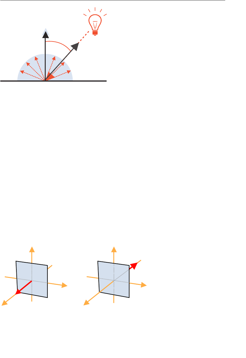
ptg11539634

Lighting 3D Objects 299

orientation of

the surface

diffuse reflection

light

direction

light

source

Figure 8.6 The light direction is from the reflecting surface to the light source

Because we aren’t using an angle to specify the orientation of the surface, we need another

mechanism to do that. The solution is to use normal vectors.

The Orientation of a Surface: What Is the Normal?

The orientation of a surface is specified by the direction perpendicular to the surface and

is called a normal or a normal vector . This direction is represented by a triple number,

which is the direction of a line from the origin (0, 0, 0) to (n

x , n

y , n

z ) specified as the

normal. For example, the direction of the normal (1, 0, 0) is the positive direction of the

x-axis, and the direction of the normal (0, 0, 1) is the positive direction of the z-axis.

When considering surfaces and their normals, two properties are important for our

discussion.

A Surface Has Two Normals

Because a surface has a front face and a back face, each side has its own normal; that is,

the surface has two normals. For example, the surface perpendicular to the z-axis has a

front face that is facing toward the positive direction of the z-axis and a back face that is

facing the negative direction of the z-axis, as shown in Figure 8.7 . Their normals are (0, 0,

1) and (0, 0, –1), respectively.

)1,0,0(lamroneht , 1)0,0(lamroneht

Figure 8.7 Normals

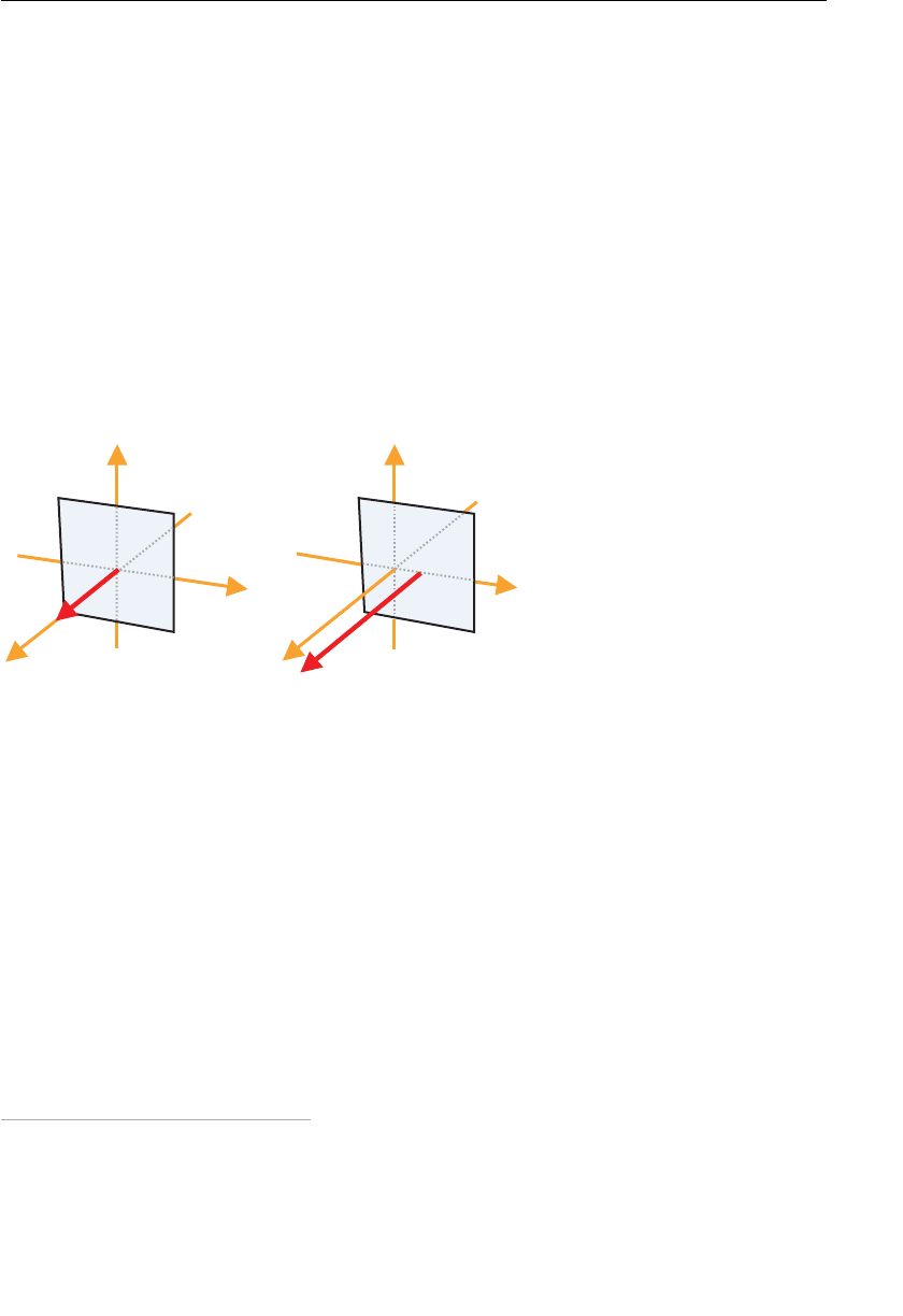
ptg11539634

CHAPTER 8 Lighting Objects

300

In 3D graphics, these two faces are distinguished by the order in which the vertices are

specified when drawing the surface. When you draw a surface specifying vertices in the

order

7 v0, v1, v2, and v3, the front face is the one whose vertices are arranged in a clock-

wise fashion when you look along the direction of the normal of the face (same as the

right-handed rule determining the positive direction of rotation in Chapter 3 , “Drawing

and Transforming Triangles”). So in Figure 8.7 , the front face has the normal (0, 0, –1) as

in the right side of the figure.

The Same Orientation Has the Same Normal

Because a normal just represents direction, surfaces with the same orientation have the

same normal regardless of the position of the surfaces.

If there is more than one surface with the same orientation placed at different positions,

the normals of these surfaces are identical. For example, the normals of a surface perpen-

dicular to the z-axis, whose center is placed at (10, 98, 9), are still (0, 0, 1) and (0, 0, –1).

They are the same as when it is positioned at the origin (see Figure 8.8 ).

)1,0,0(lamroneht )1—,0,0(lamroneht

Figure 8.8 If the orientation of the surface is the same, the normal is identical regardless of

its position

The left side of Figure 8.9 shows the normals that are used in the sample programs in this

section. Normals are labeled using, for example “n(0, 1, 0)” as in this figure.

7 Actually, this surface is composed of two triangles: a triangle drawn in the order v0, v1, and v2, and a

triangle drawn in the order v0, v2, and v3.

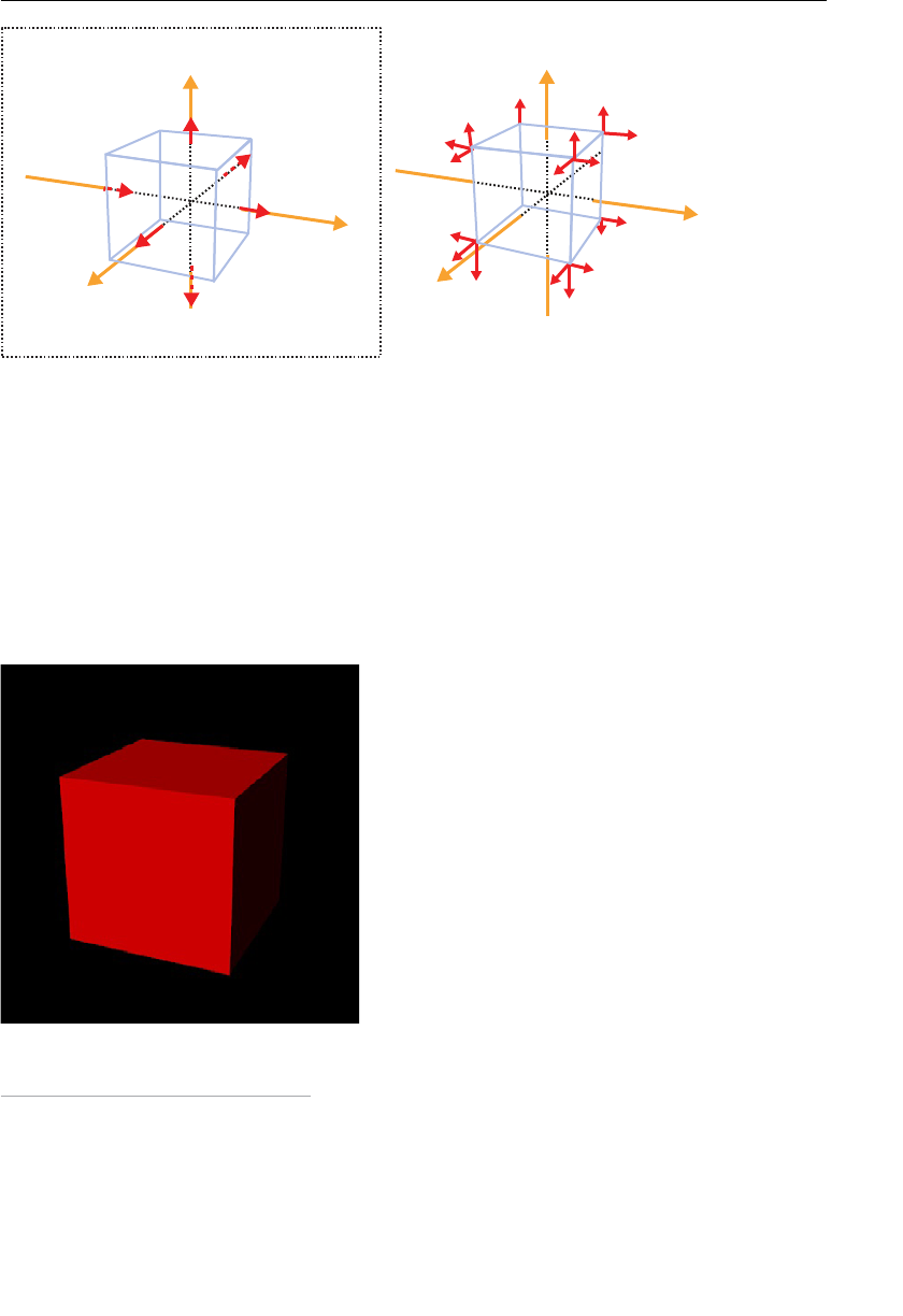
ptg11539634

Lighting 3D Objects 301

)1,0,0(n

)0,1,0(n

)0,0,1(n

)0,0,1—(n

)1—,0,0(n

)0,0,1(n

).deyalpsidtoneraslamronlla(

)0,1—,0(n

v4(1,-1,-1) v4(1,-1,-1)

v3(1,-1,1) v3(1,-1,1)

v2(-1,-1,1) v2(-1,-1,1)

v7(-1,-1,-1)

v0(1, 1, 1)

v1(-1,1,1)

v6(-1, 1,-1) v6(-1, 1,-1)

v5(1, 1,-1) v5(1, 1,-1)

v0(1, 1, 1)

v7(-1,-1,-1)

)1,0,(n0

)0,1,0(n

Figure 8.9 Normals of the surfaces of a cube

Once you have calculated the normals for a surface, the next task is to pass that data to

the shader programs. In the previous chapter, you passed color data for a surface to the

shader as “per-vertex data.” You can pass normal data using the same approach: as per-

vertex data stored in a buffer object. In this section, as shown in Figure 8.9 (right side),

the normal data is specified for each vertex, and in this case there are three normals per

vertex, just as there are three color data specified per vertex.

Now let’s construct a sample program LightedCube that displays a red cube lit by a white

directional light. The result is shown in Figure 8.10 .

Figure 8.10 LightedCube

8 Cubes or cuboids are simple but special objects whose three surfaces are connected perpendicularly.

They have three different normals per vertex. On the other hand, smooth objects such as game

characters have one normal per vertex.

ptg11539634

CHAPTER 8 Lighting Objects

302

Sample Program (LightedCube.js)

The sample program is shown in Listing 8.1 . It is based on ColoredCube from the previous

chapter, so the basic processing flow of this program is the same as

ColoredCube .

As you can see from Listing 8.1 , the vertex shader has been significantly modified so that

it calculates Equation 8.4 . In addition, the normal data is added in

initVertexBuffers()

defined at line 89, so that they can be passed to the variable

a_Normal . The fragment

shader is the same as in

ColoredCube , and unmodified. It is reproduced so that you can

see that no fragment processing is needed.

Listing 8.1 LightedCube.js

1 // LightedCube.js

2 // Vertex shader program

3 var VSHADER_SOURCE =

4 ‘attribute vec4 a_Position;n’ +

5 ‘attribute vec4 a_Color;n’ +

6 ‘attribute vec4 a_Normal;n’ + // Normal

7 ‘uniform mat4 u_MvpMatrix;n’ +

8 ‘uniform vec3 u_LightColor;n’ + // Light color

9 ‘uniform vec3 u_LightDirection;n’ + // world coordinate, normalized

10 ‘varying vec4 v_Color;n’ +

11 ‘void main() {n’ +

12 ‘ gl_Position = u_MvpMatrix * a_Position ;n’ +

13 // Make the length of the normal 1.0

14 ‘ vec3 normal = normalize(vec3(a_Normal));n’ +

15 // Dot product of light direction and orientation of a surface

16 ‘ float nDotL = max(dot(u_LightDirection, normal), 0.0);n’ +

17 // Calculate the color due to diffuse reflection

18 ‘ vec3 diffuse = u_LightColor * vec3(a_Color) * nDotL;n’ +

19 ‘ v_Color = vec4(diffuse, a_Color.a);n’ +

20 ‘}n’;

22 // Fragment shader program

…

28 ‘void main() {n’ +

29 ‘ gl_FragColor = v_Color;n’ +

30 ‘}n’;

32 function main() {

…

49 // Set the vertex coordinates, the color, and the normal

50 var n = initVertexBuffers(gl);

…

ptg11539634

Lighting 3D Objects 303

61 var u_MvpMatrix = gl.getUniformLocation(gl.program, ‘u_MvpMatrix’);

62 var u_LightColor = gl.getUniformLocation(gl.program, ‘u_LightColor’);

63 var u_LightDirection = gl.getUniformLocation(gl.program, ‘u_LightDirection’);

…

69 // Set the light color (white)

70 gl.uniform3f(u_LightColor, 1.0, 1.0, 1.0);

71 // Set the light direction (in the world coordinate)

72 var lightDirection = new Vector3([0.5, 3.0, 4.0]);

73 lightDirection.normalize(); // Normalize

74 gl.uniform3fv(u_LightDirection, lightDirection.elements);

76 // Calculate the view projection matrix

77 var mvpMatrix = new Matrix4(); // Model view projection matrix

78 mvpMatrix.setPerspective(30, canvas.width/canvas.height, 1, 100);

79 mvpMatrix.lookAt(3, 3, 7, 0, 0, 0, 0, 1, 0);

80 // Pass the model view projection matrix to the variable u_MvpMatrix

81 gl.uniformMatrix4fv(u_MvpMatrix, false, mvpMatrix.elements);

…

86 gl.drawElements(gl.TRIANGLES, n, gl.UNSIGNED_BYTE, 0);// Draw a cube

87 }

89 function initVertexBuffers(gl) {

…

98 var vertices = new Float32Array([ // Vertices

99 1.0, 1.0, 1.0, -1.0, 1.0, 1.0, -1.0,-1.0, 1.0, 1.0,-1.0, 1.0,

100 1.0, 1.0, 1.0, 1.0,-1.0, 1.0, 1.0,-1.0,-1.0, 1.0, 1.0,-1.0,

…

104 1.0,-1.0,-1.0, -1.0,-1.0,-1.0, -1.0, 1.0,-1.0, 1.0, 1.0,-1.0

105 ]);

…

117

118 var normals = new Float32Array([ // Normals

119 0.0, 0.0, 1.0, 0.0, 0.0, 1.0, 0.0, 0.0, 1.0, 0.0, 0.0, 1.0,

120 1.0, 0.0, 0.0, 1.0, 0.0, 0.0, 1.0, 0.0, 0.0, 1.0, 0.0, 0.0,

…

124 0.0, 0.0,-1.0, 0.0, 0.0,-1.0, 0.0, 0.0,-1.0, 0.0, 0.0,-1.0

125 ]);

…

140 if(!initArrayBuffer(gl,’a_Normal’, normals, 3, gl.FLOAT)) return -1;

…

154 return indices.length;

155 }

ptg11539634

CHAPTER 8 Lighting Objects

304

As a reminder, here is the calculation that the vertex shader performs ( Equation 8.4 ):

()

〈〉=

〈〉×〈〉×

〈〉〈 〉

surface color by diffuse reflection

light color base color of surface

light direction orientation of a surface

 



i

You can see that four pieces of information are needed to calculate this equation: (1) light

color, (2) a surface base color, (3) light direction, and (4) surface orientation. In addition,

<light direction> and <surface orientation> must be normalized (1.0 in length).

Processing in the Vertex Shader

From the four pieces of information necessary for Equation 8.4 , the base color of a

surface is passed as

a_Color at line 5 in the following code, and the surface orientation is

passed as

a_Normal at line 6. The light color is passed using u_LightColor at line 8, and

the light direction is passed as

u_LightDirection at line 9. You should note that only

u_LightDirection is passed in the world coordinate

9 system and has been normalized in

the JavaScript code for ease of handling. This avoids the overhead of normalizing it every

time it’s used in the vertex shader:

4 ‘attribute vec4 a_Position;n’ +

5 ‘attribute vec4 a_Color;n’ + <-(2) surface base color

6 ‘attribute vec4 a_Normal;n’ + // Normal <-(4) surface orientation

7 ‘uniform mat4 u_MvpMatrix;n’ +

8 ‘uniform vec3 u_LightColor;n’ + // Light color <-(1)

9 ‘uniform vec3 u_LightDirection;n’ + // world coordinate,normalized <-(3)

10 ‘varying vec4 v_Color;n’ +

11 ‘void main() {n’ +

12 ‘ gl_Position = u_MvpMatrix * a_Position ;n’ +

13 // Make the length of the normal 1.0

14 ‘ vec3 normal = normalize(vec3(a_Normal));n’ +

15 // Dot product of light direction and orientation of a surface

16 ‘ float nDotL = max(dot(u_LightDirection, normal), 0.0);n’ +

17 // Calculate the color due to diffuse reflection

18 ‘ vec3 diffuse = u_LightColor * vec3(a_Color) * nDotL;n’ +

19 ‘ v_Color = vec4(diffuse, a_Color.a);n’ +

20 ‘}n’;

Once the necessary information is available, you can carry out the calculation. First, the

vertex shader normalizes the vector at line 14. Technically, because the normal used in

this sample program is 1.0 in length, this process is not necessary. However, it is good

practice, so it is performed here:

9 In this book, the light effect with shading is calculated in the world coordinate system (see Appendix

G , “World Coordinate System Versus Local Coordinate System”) because it is simpler to program and

more intuitive with respect to the light direction. It is also safe to calculate it in the view coordinate

system but more complex.

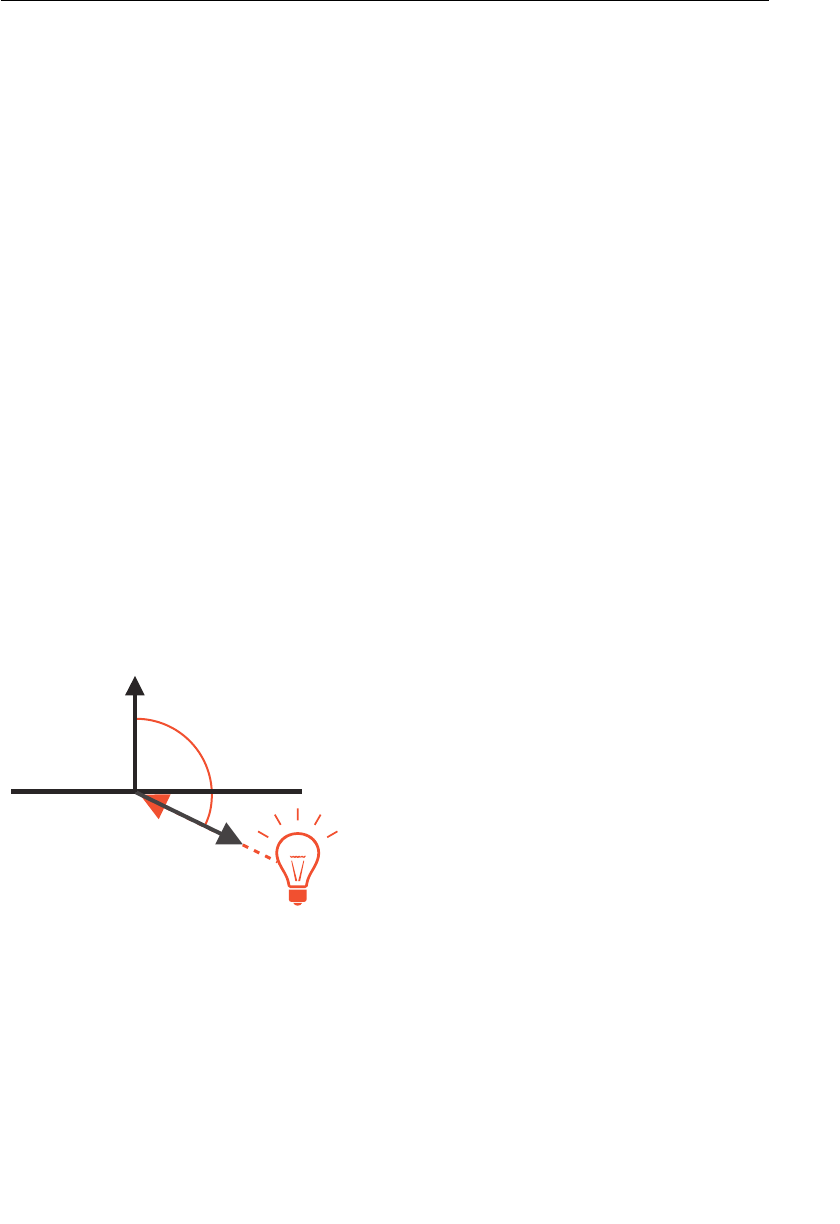
ptg11539634

Lighting 3D Objects 305

14 ‘ vec3 normal = normalize(vec3(a_Normal));n’ +

Although a_Normal is of type vec4 , a normal represents a direction and uses only the x, y,

and z components. So you extract these components with .

xyz and then normalize. If you

pass the normal using a type

vec3 , this process is not necessary. However, it is passed as

a type

vec4 in this code because a vec4 will be needed when we extend the code for the

next example. We will explain the details in a later sample program. As you can see, GLSL

ES provides

normalize() , a built-in function to normalize a vector specified as its argu-

ment. In the program, the normalized normal is stored in the variable

normal for use later.

Next, you need to calculate the dot product 〈〉〈 〉light direction surface orientationi from

Equation 8.4 . The light direction is stored in

u_LightDirection . Because it is already

normalized, you can use it as is. The orientation of the surface is the

normal that was

normalized at line 14. The dot product “ · ” can then be calculated using the built-in

function

dot() , which again is provided by GLSL ES and returns the dot product of the

two vectors specified as its arguments. That is, calling

dot(u_LightDirection, normal)

performs 〈〉〈 〉light direction surface orientationi . This calculation is performed at line 16.

16 ‘ float nDotL = max(dot(u_LightDirection, normal), 0.0);n’ +

Once the dot product is calculated, if the result is positive, it is assigned to nDotL . If it is

negative then 0.0 is assigned. The function

max() used here is a GLSL ES built-in function

that returns the greater value from its two arguments.

A negative dot product means that

in cos

is more than 90 degrees. Because

is the

angle between the light direction and the surface orientation, a value of

greater than 90

degrees means that light hits the surface on its back face (see Figure 8.11 ). This is the same

as no light hitting the front face, so 0.0 is assigned to

nDotL .

θ09>

orientation of

the surface

diffuse reflection

light

direction

light

source

Figure 8.11 A normal and light in case

is greater than 90 degrees

Now that the preparation is completed, you can calculate Equation 8.4 . This is performed

at line 18, which is a direct implementation of Equation 8.4 . a_Color , which is of type

vec4 and holds the RGBA values, is converted to a vec3 ( .rgb ) because its transparency

(alpha value) is not used in lighting.

ptg11539634

CHAPTER 8 Lighting Objects

306

In fact, transparency of an object’s surface has a significant effect on the color of the

surface. However, because the calculation of the light passing through an object is compli-

cated, we ignore transparency and don’t use the alpha value in this program:

18 ‘ vec3 diffuse = u_LightColor * vec3(a_Color) * nDotL;n’ +

Once calculated, the result, diffuse , is assigned to the varying variable v_Color at line 19.

Because

v_Color is of type vec4 , diffuse is also converted to vec4 with 1.0 :

19 ‘ v_Color = vec4(diffuse, 1.0);n’ +

The result of the processing steps above is that a color, depending on the direction of

the vertex’s normal, is calculated, passed to the fragment shader, and assigned to

gl_

FragColor . In this case, because you use a directional light, vertices that make up the same

surface are the same color, so each surface will be a solid color.

That completes the vertex shader code. Let’s now take a look at how the JavaScript

program passes the data needed for Equation 8.4 to the vertex shader.

Processing in the JavaScript Program

The light color (

u_LightColor ) and the light direction ( u_LightDirection ) are passed to

the vertex shader from the JavaScript program. Because the light color is white (1.0, 1.0,

1.0), it is simply written to

u_LightColor using gl.uniform3f() :

69 // set the Light color (white)

70 gl.uniform3f(u_LightColor, 1.0, 1.0, 1.0);

The next step is to set up the light direction, which must be passed after normalization, as

discussed before. You can normalize it with the

normalize() function for Vector3 objects

that is provided in

cuon-matrix.js . Usage is simple: Create the Vector3 object that speci-

fies the vector you want to normalize as its argument (line 72), and invoke the

normal-

ize() method on the object. Note that the notation in JavaScript is different from that of

GLSL ES:

71 // Set the light direction (in the world coordinate)

72 var lightDirection = new Vector3([0.5, 3.0, 4.0]);

73 lightDirection.normalize(); // Normalize

74 gl.uniform3fv(u_LightDirection, lightDirection.elements);

The result is stored in the elements property of the object in an array of type

Float32Array and then assigned to u_LightDirection using gl.uniform3fv() (line 74).

Finally, the normal data is written in initVertexBuffers(), defined at line 89. Actual

normal data is stored in the array

normals at line 118 per vertex along with the color

data, as in

ColoredCube.js . Data is assigned to a_Normal in the vertex shader by invoking

initArrayBuffer() at line 140:

140 if(!initArrayBuffer(gl, ‘a_Normal’, normals, 3, gl.FLOAT)) return -1;

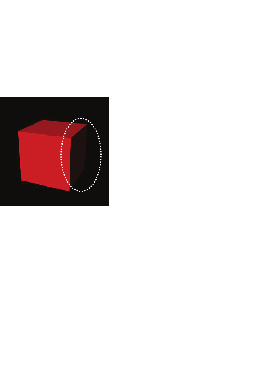
ptg11539634

Lighting 3D Objects 307

initArrayBuffer() , which was also used in ColoredCube , assigns the array specified by

the third argument (

normals ) to the attribute variable that has the name specified by the

second argument (

a_Normal ).

Add Shading Due to Ambient Light

Although at this stage you have successfully added lighting to the scene, as you can see

from Figure 8.9 , when you run

LightedCube , the cube is a little different from the box in

the real world. In particular, the surface on the opposite side of the light source appears

almost black and not clearly visible. You can see this problem more clearly if you animate

the cube. Try the sample program

LightedCube_animation (see Figure 8.12 ) to see the

problem more clearly.

Figure 8.12 The result of LightedCube_animation

Although the scene is correctly lit as the result of Equation 8.4 , our real-world experiences

tells us that something isn’t right. It is unusual to see such a sharp effect because, in the

real world, surfaces such as the back face of the cube are also lit by diffuse or reflected

light. The ambient light described in the previous section represents this indirect light

and can be used to make the scene more lifelike. Let’s add that to the scene and see if the

effect is more realistic. Because ambient light models the light that hits an object from all

directions with constant intensity, the surface color due to the reflection is determined

only by the light color and the base color of the surface. The formula that calculates this

was shown as Equation 8.2 . Let’s see it again:

〈〉=

〈〉×〈〉

surface color by ambient reflection

light color base color of surface

 



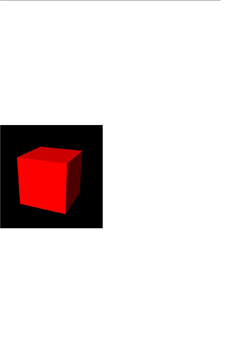
ptg11539634

CHAPTER 8 Lighting Objects

308

Let’s try to add the color due to ambient light described by this formula to the sample

program

LightedCube . To do this, use Equation 8.3 shown here:

〈〉=

〈〉+〈〉

surface color by diffuse and ambient reflection

surface color by diffuse reflection surface color by ambient reflection

  

   

Ambient light is weak because it is the light reflected by other objects like the walls. For

example, if the ambient light color is (0.2, 0.2, 0.2) and the base color of a surface is red,

or (1.0, 0.0, 0.0), then, from Equation 8.2 , the surface color due to the ambient light is

(0.2, 0.0, 0.0). For example, if there is a white box in a blue room—that is, the base color

of the surface is (1.0, 1.0, 1.0) and the ambient light is (0.0, 0.0, 0.2)—the color becomes

slightly blue (0.0, 0.0, 0.2).

Let’s implement the effect of ambient reflection in the sample program

LightedCube_

ambient , which results in the cube shown in Figure 8.13 . You can see that the surface that

the light does not directly hit is now also slightly colored and more closely resembles the

cube in the real world.

Figure 8.13 LightedCube_ambient

Sample Program (LightedCube_ambient.js)

Listing 8.2 illustrates the sample program. Because it is almost the same as LightedCube ,

only the modified parts are shown.

Listing 8.2 LightedCube_ambient.js

1 // LightedCube_ambient.js

2 // Vertex shader program

…

ptg11539634

Lighting 3D Objects 309

8 ‘uniform vec3 u_LightColor;n’ + // Light color

9 ‘uniform vec3 u_LightDirection;n’ + // World coordinate, normalized

10 ‘uniform vec3 u_AmbientLight;n’ + // Color of an ambient light

11 ‘varying vec4 v_Color;n’ +

12 ‘void main() {n’ +

…

16 // The dot product of the light direction and the normal

17 ‘ float nDotL = max(dot(lightDirection, normal), 0.0);n’ +

18 // Calculate the color due to diffuse reflection

19 ‘ vec3 diffuse = u_LightColor * a_Color.rgb * nDotL;n’ +

20 // Calculate the color due to ambient reflection

21 ‘ vec3 ambient = u_AmbientLight * a_Color.rgb;n’ +

22 // Add surface colors due to diffuse and ambient reflection

23 ‘ v_Color = vec4(diffuse + ambient, a_Color.a);n’ +

24 ‘}n’;

…

36 function main() {

…

64 // Get the storage locations of uniform variables and so on

…

68 var u_AmbientLight = gl.getUniformLocation(gl.program, ‘u_AmbientLight’);

…

80 // Set the ambient light

81 gl.uniform3f(u_AmbientLight, 0.2, 0.2, 0.2);

…

95 }

u_AmbientLight at line 10 is added to the vertex shader to pass in the color of ambient

light. After Equation 8.2 is calculated using it and the base color of the surface (

a_Color ),

the result is stored in the variable ambient (line 21). Now that both

diffuse and ambient

are determined, the surface color is calculated at line 23 using Equation 8.3 . The result is

passed to

v_Color , just like in LightedCube , and the surface is painted with this color.

As you can see, this program simply adds ambient at line 23, causing the whole cube to

become brighter. This implements the effect of the ambient light hitting an object equally

from all directions.

The examples so far have been able to handle static objects. However, because objects are

likely to move within a scene, or the viewpoint changes, you have to be able to handle

such transformations. As you will recall from Chapter 4 , “More Transformations and Basic

Animation,” an object can be translated, scaled, or rotated using coordinate transforma-

tions. These transformations may also change the normal direction and require a recalcu-

lation of lighting as the scene changes. Let’s take a look at how to achieve that.

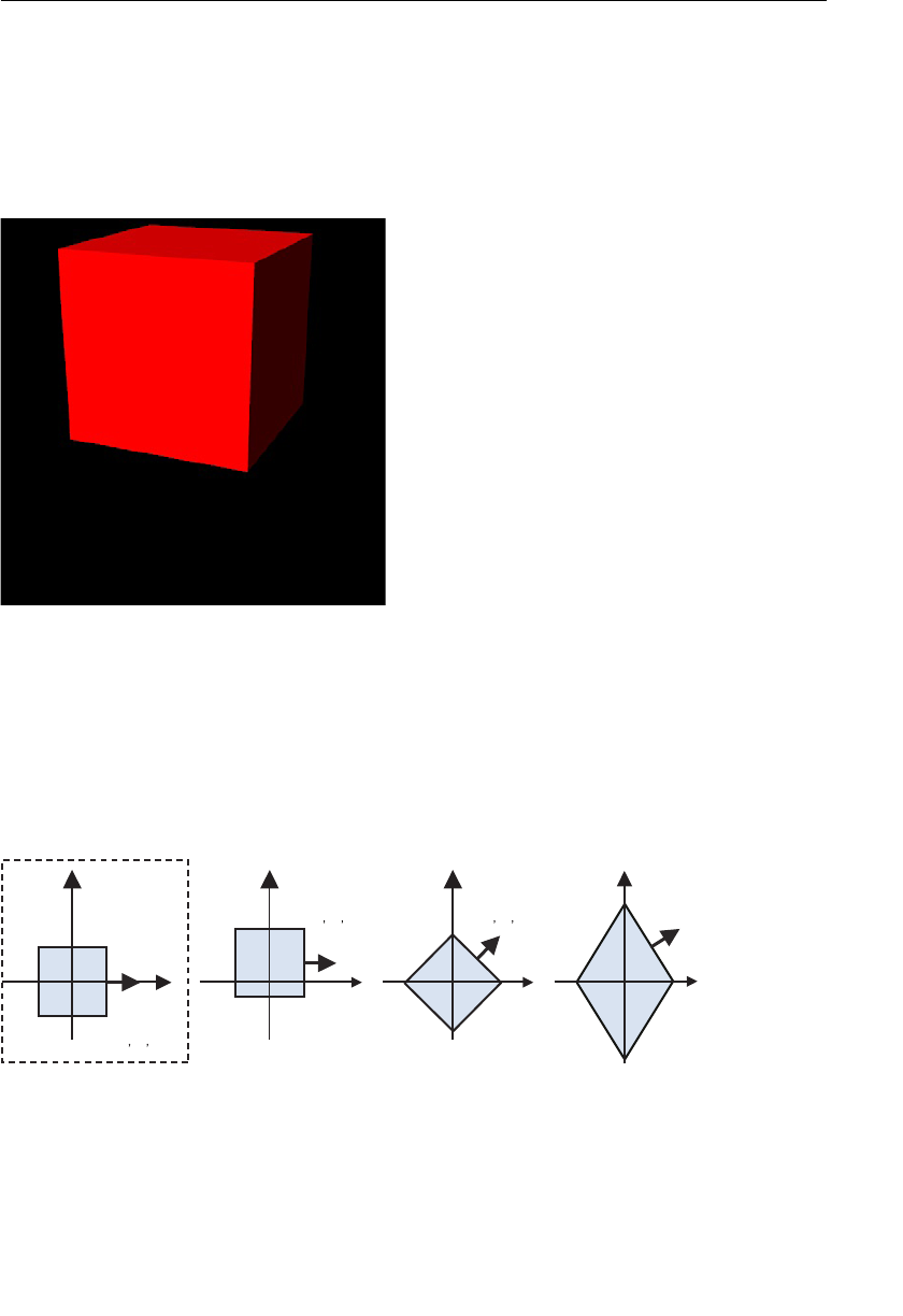
ptg11539634

CHAPTER 8 Lighting Objects

310

Lighting the Translated—Rotated Object

The program LightedTranslatedRotatedCube uses a directional light source to light a cube

that is rotated 90 degrees clockwise around the z-axis and translated 0.9 units in the y-axis

direction. A part from a directional light as described in the previous section, the sample,

LightedCube_ambient , uses diffuse reflection and ambient reflection and rotates and trans-

lates the cube. The result is shown in Figure 8.14 .

Figure 8.14 LightedTranslatedRotatedCube

You saw in the previous section that the normal direction may change when coordinate

transformations are applied. Figure 8.15 shows some examples of that. The leftmost figure

in Figure 8.15 shows the cube used in this sample program looking along the negative

direction of the z-axis. The only normal (1, 0, 0), which is toward the positive direction of

the x-axis, is shown. Let’s perform some coordinate transforms on this figure, which are

the three figures on the right.

lamroneht

noitcerid

1( 0)0

noitceridlamroneht

1( 0)0

noitceridlamroneht

1( 1)0

noitceridlamroneht

)0,5.0,1(

noitalsnart)1(

)sixa—yehtgnolaetalsnart(

noitator)2(

)seerged54etator(

gnilacs)3(

gnola2ybelacs(

)sixa—yeht

lamronlanigiroeht

Figure 8.15 The changes of the normal direction due to coordinate transformations

ptg11539634

Lighting the Translated-Rotated Object 311

You can see the following from Figure 8.15 :

• The normal direction is not changed by a translation because the orientation of the

object does not change.

• The normal direction is changed by a rotation according to the orientation of the

object.

• Scaling has a more complicated effect on the normal. As you can see, the object in

the rightmost figure is rotated i and then scaled two times only in the y-axis. In

this case, the normal direction is changed because the orientation of the surface

changes. On the other hand, if an object is scaled equally in all axes the normal

direction is not changed. Finally, even if an object is scaled unequally, the normal

direction may not change . For example, when the leftmost figure (the original

normal) is scaled two times only in the y-axis direction, the normal direction does

not change.

Obviously, the calculation of the normal under various transformations is complex, partic-

ularly when dealing with scaling. However, a mathematical technique can help.

The Magic Matrix: Inverse Transpose Matrix

As described in Chapter 4 , the matrix that performs a coordinate transformation on an

object is called a model matrix. The normal direction can be calculated by multiplying the

normal by the inverse transpose matrix of a model matrix. The inverse transpose matrix

is the matrix that transposes the inverse of a matrix.

The inverse of the matrix M is the matrix R, where both R*M and M*R become the iden-

tity matrix. The term transpose means the operation that exchanges rows and columns of

a matrix. The details of this are explained in Appendix E , “The Inverse Transpose Matrix.”

For our purposes, it can be summarized simply using the following rule:

Rule: You can calculate the normal direction if you multiply the normal by the

inverse transpose of the model matrix.

The inverse transpose matrix is calculated as follows:

1. Invert the original matrix.

2. Transpose the resulting matrix.

This can be carried out using convenient methods supported by the

Matrix4 object (see

Table 8.1 ).

ptg11539634

CHAPTER 8 Lighting Objects

312

Table 8.1 Matrix4 Methods for an Inverse Transpose Matrix

Method Description

Matrix4.setInverseOf(m) Calculates the inverse of the matrix stored in m and stores the

result in the

Matrix4 object, where m is a Matrix4 object

Matrix4.transpose() Transposes the matrix stored in the Matrix4 object and writes

the result back into the

Matrix4 object

Assuming that a model matrix is stored in

modelMatrix , which is a Matrix4 object, the

following code snippet will get its inverse transpose matrix. The result is stored in the vari-

able named

normalMatrix , because it performs the coordinate transformation of a normal:

Matrix4 normalMatrix = new Matrix4();

// Calculate the model matrix

…

// Calculate the matrix to transform normal according to the model matrix

normalMatrix.setInverseOf(modelMatrix);

normalMatrix.transpose();

Now let’s see the program LightedTranslatedRotatedCube.js that lights the cube, which

is rotated 90 degrees clockwise around the z-axis and translated 0.9 along the y-axis, all

using directional light. You’ll use the cube that was transformed by the model matrix in

LightedCube_ambient from the previous section.

Sample Program (LightedTranslatedRotatedCube.js)

Listing 8.3 shows the sample program. The changes from LightedCube_ambient are that

u_NormalMatrix is added (line to pass the matrix for coordinate transformation of the

normal to the vertex shader, and the normal is transformed at line 16 using this matrix.

u_NormalMatrix is calculated within the JavaScript.

Listing 8.3 LightedTranslatedRotatedCube.js

1 // LightedTranslatedRotatedCube.js

2 // Vertex shader program

3 var VSHADER_SOURCE =

…

6 ‘attribute vec4 a_Normal;n’ +

7 ‘uniform mat4 u_MvpMatrix;n’ +

8 ‘uniform mat4 u_NormalMatrix;n’+ // Transformation matrix of normal

9 ‘uniform vec3 u_LightColor;n’ + // Light color

10 ‘uniform vec3 u_LightDirection;n’ + // World coordinate, normalized

11 ‘uniform vec3 u_AmbientLight;n’ + // Ambient light color

12 ‘varying vec4 v_Color;n’ +

ptg11539634

Lighting the Translated-Rotated Object 313

13 ‘void main() {n’ +

14 ‘ gl_Position = u_MvpMatrix * a_Position;n’ +

15 // Recalculate normal with normal matrix and make its length 1.0

16 ‘ vec3 normal = normalize(vec3(u_NormalMatrix * a_Normal));n’ +

17 // The dot product of the light direction and the normal

18 ‘ float nDotL = max(dot(u_LightDirection, normal), 0.0);n’ +

19 // Calculate the color due to diffuse reflection

20 ‘ vec3 diffuse = u_LightColor * a_Color.rgb * nDotL;n’ +

21 // Calculate the color due to ambient reflection

22 ‘ vec3 ambient = u_AmbientLight * a_Color.rgb;n’ +

23 // Add the surface colors due to diffuse and ambient reflection

24 ‘ v_Color = vec4(diffuse + ambient, a_Color.a);n’ +

25 ‘}n’;

…

37 function main() {

…

65 // Get the storage locations of uniform variables and so on

66 var u_MvpMatrix = gl.getUniformLocation(gl.program, ‘u_MvpMatrix’);

67 var u_NormalMatrix = gl.getUniformLocation(gl.program, ‘u_NormalMatrix’);

…

85 var modelMatrix = new Matrix4(); // Model matrix

86 var mvpMatrix = new Matrix4(); // Model view projection matrix

87 var normalMatrix = new Matrix4(); // Transformation matrix for normal

89 // Calculate the model matrix

90 modelMatrix.setTranslate(0, 1, 0); // Translate to y-axis direction

91 modelMatrix.rotate(90, 0, 0, 1); // Rotate around the z-axis

92 // Calculate the view projection matrix

93 mvpMatrix.setPerspective(30, canvas.width/canvas.height, 1, 100);

94 mvpMatrix.lookAt(-7, 2.5, 6, 0, 0, 0, 0, 1, 0);

95 mvpMatrix.multiply(modelMatrix);

96 // Pass the model view projection matrix to u_MvpMatrix

97 gl.uniformMatrix4fv(u_MvpMatrix, false, mvpMatrix.elements);

99 // Calculate matrix to transform normal based on the model matrix

100 normalMatrix.setInverseOf(modelMatrix);

101 normalMatrix.transpose();

102 // Pass the transformation matrix for normal to u_NormalMatrix

103 gl.uniformMatrix4fv(u_NormalMatrix, false, normalMatrix.elements);

…

110 }

ptg11539634

CHAPTER 8 Lighting Objects

314

The processing in the vertex shader is almost the same as in LightedCube_ambient . The

difference, in line with the preceding rule, is that you multiply

a_Normal by the inverse

transpose of the model matrix at line 16 instead of using it as-is:

15 // Recalculate normal with normal matrix and make its length 1.0

16 ‘ vec3 normal = normalize(vec3(u_NormalMatrix * a_Normal));n’ +

Because you passed a_Normal as type vec4 , you can multiply it by u_NormalMatrix , which

is of type

mat4 . You only need the x, y, and z components of the result of the multiplica-

tion, so the result is converted into type

vec3 with vec3() . It is also possible to use . xyz

as before, or write

(u_NormalMatrix * a_Normal).xyz . However, vec3() is used here for

simplicity. Now that you understand how the shader calculates the normal direction

resulting from the rotation and translation of the object, let’s move on to the explanation

of the JavaScript program. The key point here is the calculation of the matrix that will be

passed to

u_NormalMatrix in the vertex shader.

u_NormalMatrix is the inverse transpose of the model matrix, so the model matrix is first

calculated at lines 90 and 91. Because this program rotates an object around the z-axis

and translates it in the y-axis direction, you can use the

setTranslate() and rotate()

methods of a

Matrix4 object as described in Chapter 4 . It is at lines 100 and 101 that the

inverse transpose matrix is actually calculated. It is passed to

u_NormalMatrix in the vertex

shader at line 103, in the same way as

mvpMatrix at line 97. The second argument of gl.

uniformMatrix4f() specifies whether to transpose the matrix ( Chapter 3 ):

99 // Calculate matrix to transform normal based on the model matrix

100 normalMatrix.setInverseOf(modelMatrix);

101 normalMatrix.transpose();

102 // Pass the normal transformation matrix to u_NormalMatrix

103 gl.uniformMatrix4fv(u_NormalMatrix, false, normalMatrix.elements);

When run, the output is similar to Figure 8.14 . As you can see, the shading is the same as

LightedCube_ambient with the cube translated in the y-axis direction. That is because (1)

the translation doesn’t change the normal direction, (2) neither does the rotation by 90

degrees, because the rotation simply switches the surfaces of the cube, (3) the light direc-

tion of the directional light does not change regardless of the position of the object, and

(4) diffuse reflection reflects the light in all directions with equal intensity.

You now have a good understanding of the basics of how to implement light and shade in

3D graphics. Let’s build on this by exploring another type of light source: the point light.

Using a Point Light Object

In contrast to a directional light, the direction of the light from a point light source differs

at each position in the 3D scene (see Figure 8.16 ). So, when calculating shading, you need

to calculate the light direction at the specific position on the surface where the light hits.

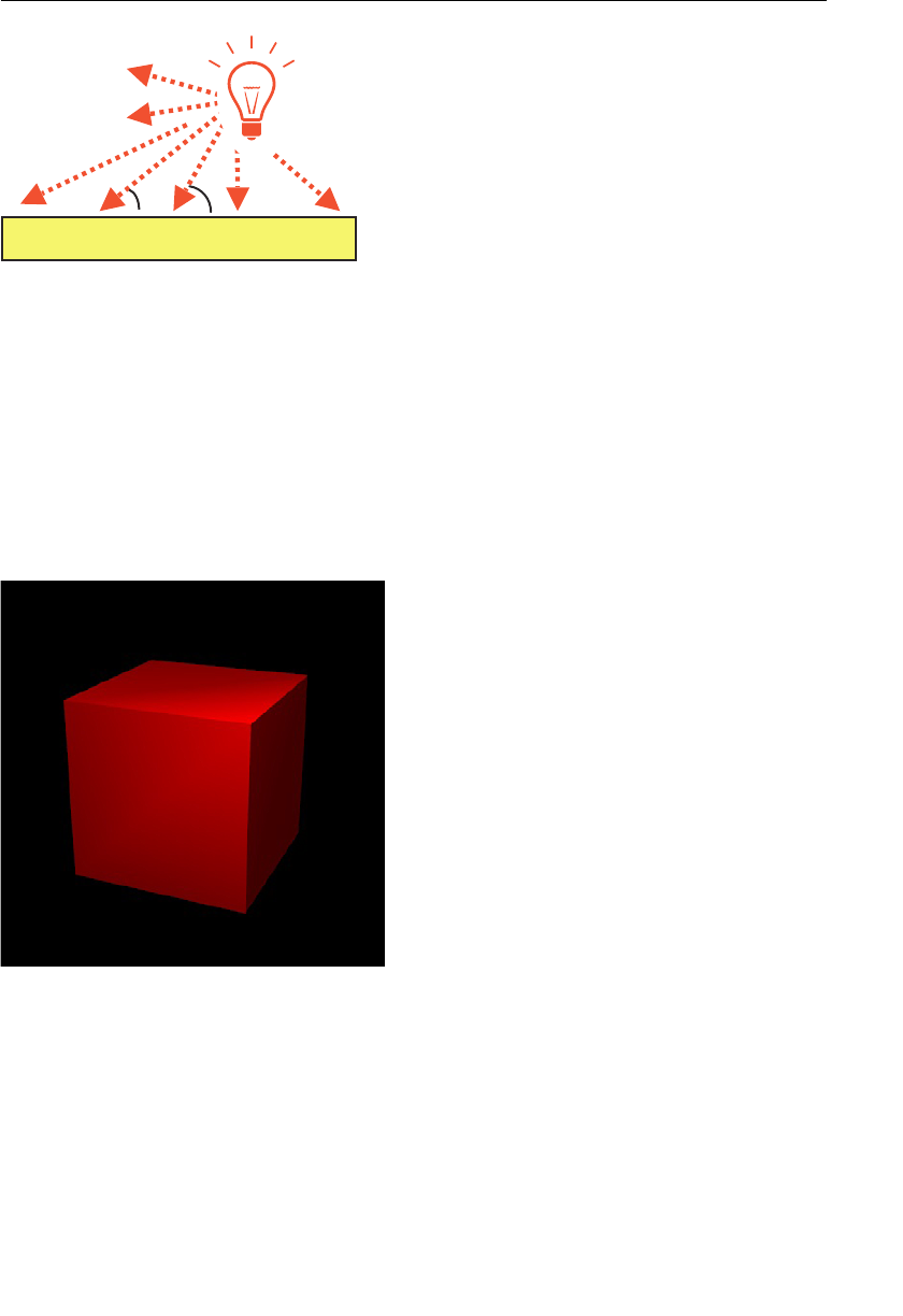
ptg11539634

Using a Point Light Object 315

αβ

a point light

Figure 8.16 The direction of a point light varies by position

In the previous sample programs, you calculated the color at each vertex by passing the

normal and the light direction for each vertex. You will use the same approach here, but

because the light direction changes, you need to pass the position of the light source and

then calculate the light direction at each vertex position.

Here, you construct the sample program

PointLightedCube that displays a red cube lit

with white light from a point light source. We again use diffuse reflection and ambient

reflection. The result is shown in Figure 8.17 , which is a version of

LightedCube_ambient

from the previous section but now lit with a point light.

Figure 8.17 PointLightedCube

Sample Program (PointLightedCube.js)

Listing 8.4 shows the sample program in which only the vertex shader is changed from

LightedCube_ambient . The variable u_ModelMatrix for passing the model matrix and the

variable

u_LightPosition representing the light position are added. Note that because you

ptg11539634

CHAPTER 8 Lighting Objects

316

use a point light in this program, you will use the light position instead of the light direc-

tion. Also, to make the effect easier to see, we have enlarged the cube.

Listing 8.4 PointLightedCube.js

1 // PointLightedCube.js

2 // Vertex shader program

3 var VSHADER_SOURCE =

4 ‘attribute vec4 a_Position;n’ +

…

8 ‘uniform mat4 u_ModelMatrix;n’ + // Model matrix

9 ‘uniform mat4 u_NormalMatrix;n’ + // Transformation matrix of normal

10 ‘uniform vec3 u_LightColor;n’ + // Light color

11 ‘uniform vec3 u_LightPosition;n’ + // Position of the light source (in the

➥world coordinate system)

12 ‘uniform vec3 u_AmbientLight;n’ + // Ambient light color

13 ‘varying vec4 v_Color;n’ +

14 ‘void main() {n’ +

15 ‘ gl_Position = u_MvpMatrix * a_Position;n’ +

16 // Recalculate normal with normal matrix and make its length 1.0

17 ‘ vec3 normal = normalize(vec3(u_NormalMatrix * a_Normal));n’ +

18 // Calculate the world coordinate of the vertex

19 ‘ vec4 vertexPosition = u_ModelMatrix * a_Position;n’ +

20 // Calculate the light direction and make it 1.0 in length

21 ‘ vec3 lightDirection = normalize(u_LightPosition – vec3(vertexPosition));n’ +

22 // The dot product of the light direction and the normal

23 ‘ float nDotL = max(dot( lightDirection, normal), 0.0);n’ +

24 // Calculate the color due to diffuse reflection

25 ‘ vec3 diffuse = u_LightColor * a_Color.rgb * nDotL;n’ +

26 // Calculate the color due to ambient reflection

27 ‘ vec3 ambient = u_AmbientLight * a_Color.rgb;n’ +

28 // Add surface colors due to diffuse and ambient reflection

29 ‘ v_Color = vec4(diffuse + ambient, a_Color.a);n’ +

30 ‘}n’;

…

42 function main() {

…

70 // Get the storage locations of uniform variables and so on

71 var u_ModelMatrix = gl.getUniformLocation(gl.program, ‘u_ModelMatrix’);

…

74 var u_LightColor = gl.getUniformLocation(gl.program,’u_LightColor’);

75 var u_LightPosition = gl.getUniformLocation(gl.program, ‘u_LightPosition’);

…

82 // Set the light color (white)

ptg11539634

Using a Point Light Object 317

83 gl.uniform3f(u_LightColor, 1.0, 1.0, 1.0);

84 // Set the position of the light source (in the world coordinate)

85 gl.uniform3f(u_LightPosition, 0.0, 3.0, 4.0);

…

89 var modelMatrix = new Matrix4(); // Model matrix

90 var mvpMatrix = new Matrix4(); // Model view projection matrix

91 var normalMatrix = new Matrix4(); // Transformation matrix for normal

93 // Calculate the model matrix

94 modelMatrix.setRotate(90, 0, 1, 0); // Rotate around the y-axis

95 // Pass the model matrix to u_ModelMatrix

96 gl.uniformMatrix4fv(u_ModelMatrix, false, modelMatrix.elements);

…

The key differences in the processing within the vertex shader are at line 19 and 21. At

line 19, you transform the vertex coordinates into world coordinates in order to calculate

the light direction at the vertex coordinates. Because a point light emits light in all direc-

tions from its position, the light direction at a vertex is the result of subtracting the vertex

position from the light source position. Because the light position is passed to the variable

u_LightPosition using world coordinates at line 11, you also have to convert the vertex

coordinates into world coordinates to calculate the light direction. The light direction

is then calculated at line 21. Note that it is normalized with

normalize() so that it will

be 1.0 in length. Using the resulting light direction (

lightDirection ), the dot product is

calculated at line 23 and then the surface color at each vertex is calculated based on this

light direction.

If you run this program, you will see a more realistic result, as shown in Figure 8.17 .

Although this result is more realistic, a closer look reveals an artifact: There are unnatural

lines of shade on the cube’s surface (see Figure 8.18 ). You can see this more easily if the

cube rotates as it does when you load

PointLightedCube_animation .

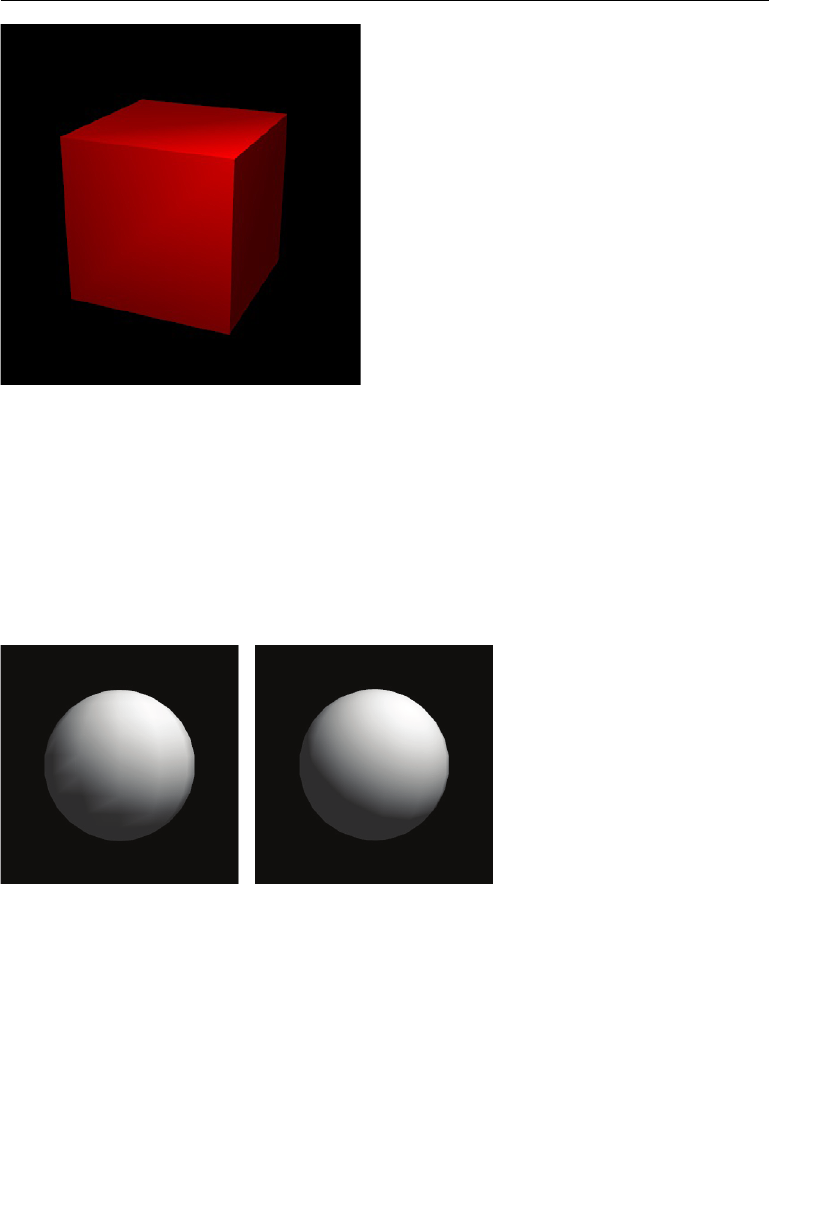
ptg11539634

CHAPTER 8 Lighting Objects

318

Figure 8.18 The unnatural appearance when processing the point light at each vertex

This comes about because of the interpolation process discussed in Chapter 5 , “Using

Colors and Texture Images.” As you will remember, the WebGL system interpolates the

colors between vertices based on the colors you supply at the vertices. However, because

the direction of light from a point light source varies by position to shade naturally, you

have to calculate the color at every position the light hits instead of just at each vertex.

You can see this problem more clearly using a sphere illuminated by a point light, as

shown in Figure 8.19 .

per-vertex

calculation

per-position

calculation

Figure 8.19 The spheres illuminated by a point light

As you can see, the border between the brighter parts and darker parts is unnatural in the

left figure. If the effect is hard to see on the page, the left figure is

PointLightedSphere ,

and the right is

PointLightedSphere_perFragment . We will describe how to draw them

correctly in the next section.

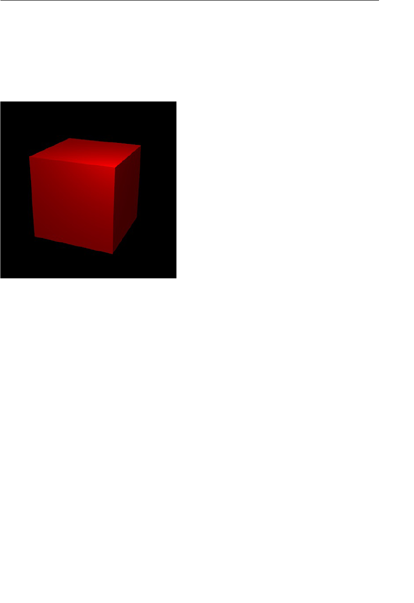
ptg11539634

Using a Point Light Object 319

More Realistic Shading: Calculating the Color per Fragment

At first glance, it may seem daunting to have to calculate the color at every position on a

cube surface where the light hits. However, essentially it means calculating the color per

fragment, so the power of the fragment shader can now be used.

This sample program you will use is

PointLightedCube_perFragment , and its result is

shown in Figure 8.20 .

Figure 8.20 PointLightedCube_perFragment

Sample Program (PointLightedCube_perFragment.js)

The sample program, which is based on PointLightedCube.js , is shown in Listing 8.5 .

Only the shader code has been modified and, as you can see, there is less processing in the

vertex shader and more processing in the fragment shader.

Listing 8.5 PointLightedCube_perFragment.js

1 // PointLightedCube_perFragment.js

2 // Vertex shader program

3 var VSHADER_SOURCE =

4 ‘attribute vec4 a_Position;n’ +

…

8 ‘uniform mat4 u_ModelMatrix;n’ + // Model matrix

9 ‘uniform mat4 u_NormalMatrix;n’ + // Transformation matrix of normal

10 ‘varying vec4 v_Color;n’ +

11 ‘varying vec3 v_Normal;n’ +

12 ‘varying vec3 v_Position;n’ +

13 ‘void main() {n’ +

ptg11539634

CHAPTER 8 Lighting Objects

320

14 ‘ gl_Position = u_MvpMatrix * a_Position;n’ +

15 // Calculate the vertex position in the world coordinate

16 ‘ v_Position = vec3(u_ModelMatrix * a_Position);n’ +

17 ‘ v_Normal = normalize(vec3(u_NormalMatrix * a_Normal));n’ +

18 ‘ v_Color = a_Color;n’ +

19 ‘}n’;

21 // Fragment shader program

22 var FSHADER_SOURCE =

…

26 ‘uniform vec3 u_LightColor;n’ + // Light color

27 ‘uniform vec3 u_LightPosition;n’ + // Position of the light source

28 ‘uniform vec3 u_AmbientLight;n’ + // Ambient light color

29 ‘varying vec3 v_Normal;n’ +

30 ‘varying vec3 v_Position;n’ +

31 ‘varying vec4 v_Color;n’ +

32 ‘void main() {n’ +

33 // Normalize normal because it’s interpolated and not 1.0 (length)

34 ‘ vec3 normal = normalize(v_Normal);n’ +

35 // Calculate the light direction and make it 1.0 in length

36 ‘ vec3 lightDirection = normalize(u_LightPosition — v_Position);n’ +

37 // The dot product of the light direction and the normal

38 ‘ float nDotL = max(dot( lightDirection, normal), 0.0);n’ +

39 // Calculate the final color from diffuse and ambient reflection

40 ‘ vec3 diffuse = u_LightColor * v_Color.rgb * nDotL;n’ +

41 ‘ vec3 ambient = u_AmbientLight * v_Color.rgb;n’ +

42 ‘ gl_FragColor = vec4(diffuse + ambient, v_Color.a);n’ +

43 ‘}n’;

To calculate the color per fragment when light hits, you need (1) the position of the frag-

ment in the world coordinate system and (2) the normal direction at the fragment posi-

tion. You can utilize interpolation ( Chapter 5 ) to obtain these values per fragment by just

calculating them per vertex in the vertex shader and passing them via varying variables to

the fragment shader.

These calculations are performed at lines 16 and 17, respectively, in the vertex shader. At

line 16, the vertex position in world coordinates is calculated by multiplying each vertex

coordinate by the model matrix. After assigning the vertex position to the varying vari-

able

v_Position , it will be interpolated between vertices and passed to the corresponding

variable (

v_Position ) in the fragment shader as the world coordinate of the fragment. The

normal calculation at line 17 is carried out for the same purpose.

10 By assigning the result

v_Normal , it is also interpolated and passed to the corresponding variable ( v_Normal ) in

the fragment shader as the normal of the fragment.

ptg11539634

Summary 321

Processing in the fragment shader is the same as that in the vertex shader of

PointLightedCube.js . First, at line 34, the interpolated normal passed from the vertex

shader is normalized. Its length may not be 1.0 anymore because of the interpolation.

Next, at line 36, the light direction is calculated and normalized. Using these results, the

dot product of the light direction and the normal is calculated at line 38. The colors due

to the diffuse reflection and ambient reflection are calculated at lines 40 and 41 and added

to get the fragment color, which is assigned to

gl_FragColor at line 42.

If you have more than one light source, after calculating the color due to diffuse reflec-

tion and ambient reflection for each light source, you can obtain the final fragment color

by adding all the colors. In other words, you only have to calculate Equation 8.3 as many

times as the number of light sources.

Summary

This chapter explored how to light a 3D scene, the different types of light used, and how

light is reflected and diffused through the scene. Using this knowledge, you then imple-

mented the effects of different light sources to illuminate a 3D object and examined

various shading techniques to improve the realism of the objects. As you have seen, a

mastery of lighting is essential to adding realism to 3D scenes, which can appear flat and

uninteresting if they’re not correctly lit.

10 In this sample program, this normalization is not necessary because all normals are passed to

a_Normal with a length of 1.0. However, we normalize them here as good programming practice so

the code is more generic.

ptg11539634

This page intentionally left blank

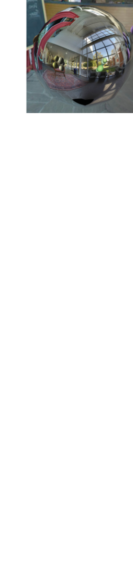
ptg11539634

This chapter is the final one that describes the core features and how to program

with WebGL. Once you’ve read it, you will have mastered the basics of WebGL

and will have enough knowledge to create realistic and interactive 3D scenes.

This chapter focuses on hierarchical objects, which are important because

they allow you to progress beyond single objects like cubes or blocks to more

complex objects that you can use for game characters, robots, and even humans.

The following key points are discussed in this chapter:

• Modeling complex connected structures such as a robot arm using a hierar-

chical structure.

• Drawing and manipulating hierarchical objects made up of multiple

simpler objects.

• Combining model and rotation matrices to mimic joints such as elbow or

wrist joints

• Internally implementing initShaders() , which you’ve used but not exam-

ined so far.

By the end of this chapter, you will have all the knowledge you need to create

compelling 3D scenes populated by both simple and complex 3D objects.

Chapter 9

Hierarchical Objects

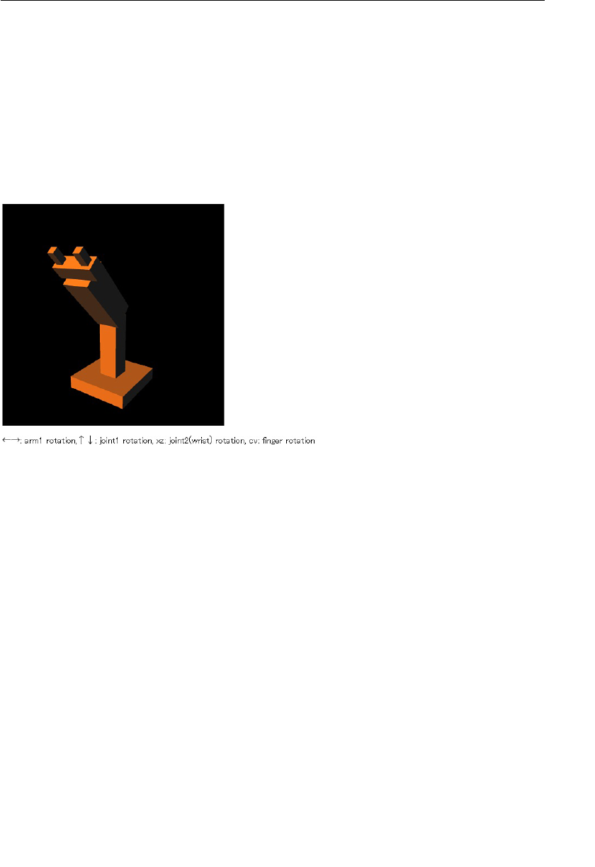
ptg11539634

CHAPTER 9 Hierarchical Objects

324

Drawing and Manipulating Objects Composed of

Other Objects

Until now, we have described how to translate and rotate a single object, such as a two-

dimensional triangle or a three-dimensional cube. But many of the objects in 3D graphics,

game characters, robots, and so on, consist of more than one object (or segment). For a

simple example, a robot arm is shown in Figure 9.1 . As you can see, this consists of multi-

ple boxes. The program name is

MultiJointModel . First, let’s load the program and experi-

ment by pressing the arrow, x, z, c, and v keys to understand what you will construct in

the following sections.

Figure 9.1 A robot arm consisting of multiple objects

One of the key issues when drawing an object consisting of multiple objects (segments)

is that you have to program to avoid conflicts when the segments move. This section will

explore this issue by describing how to draw and manipulate a robot arm that consists

of multiple segments. First, let’s consider the structure of the human body from the

shoulder to the fingertips to understand how to model our robot arm. An arm consists of

multiple segments, such as the upper arm, lower arm, palm, and fingers, each of which is

connected by a joint, as shown on the left of Figure 9.2 .

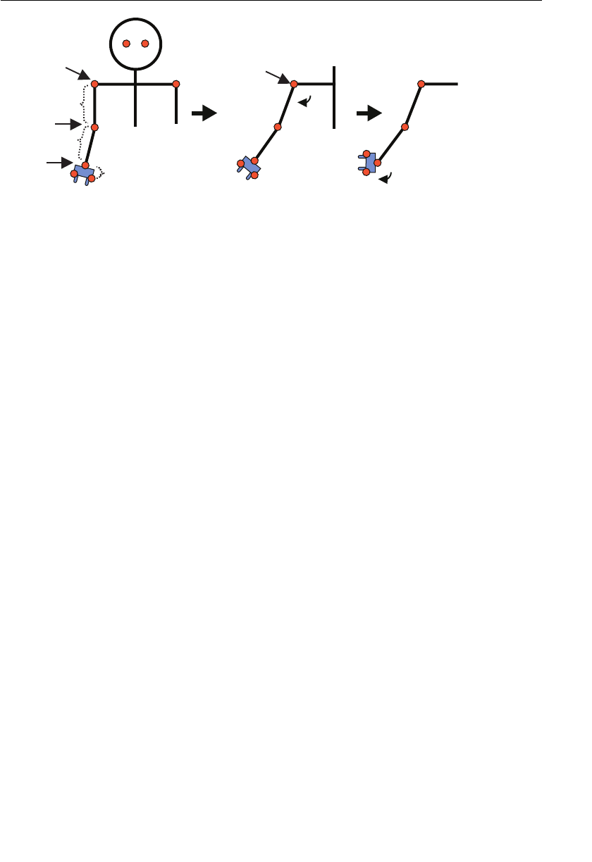
ptg11539634

Drawing and Manipulating Objects Composed of Other Objects 325

mrareppu

mlap

tniojwoble

tniojredluohs

tniojredluohsehtetator

tniojtsirw

tniojtsirwehtetator

tniojredluohs

mrarewol

mrareppu

mlap

finger1

finger2

finger1 finger2

Figure 9.2 The structure and movement from the arm to the fingers

Each segment moves around a joint as follows:

• When you move the upper arm by rotating around the shoulder joint, depending

on the upper arm movement, the lower arm, palm, and fingers move (the middle of

Figure 9.2 ) accordingly.

• When you move the lower arm using an elbow joint, the palm and fingers move but

the upper arm does not.

• When you move the palm using the wrist joint, both palm and fingers move but the

upper and lower arm do not (the right of Figure 9.2 ).

• When you move fingers, the upper arm, lower arm, and palm do not move.

To summarize, when you move a segment, the segments located below it move, while the

segments located above are not affected. In addition, all movement, including twisting, is

actually rotation around a joint.

Hierarchical Structure

The typical method used to draw and manipulate the object with such features is to draw

each part object (such as a box) in the order of the object’s hierarchical structure from

upper to lower, applying each model matrix (rotation matrix) at every joint. For example,

in Figure 9.2 , shoulder, elbow, wrist, and finger joints all have respective rotation matrices.

It is important to note that, unlike humans or robots, segments in 3D graphics are not

physically joined. So if you inadvertently rotate the object corresponding to an upper arm

at the shoulder joint, the lower parts would be left behind. When you rotate the shoulder

joint, you should explicitly make the lower parts follow the movement. To do this, you

need to rotate the lower elbow and wrist joints through the same angle that you rotate the

shoulder joint.

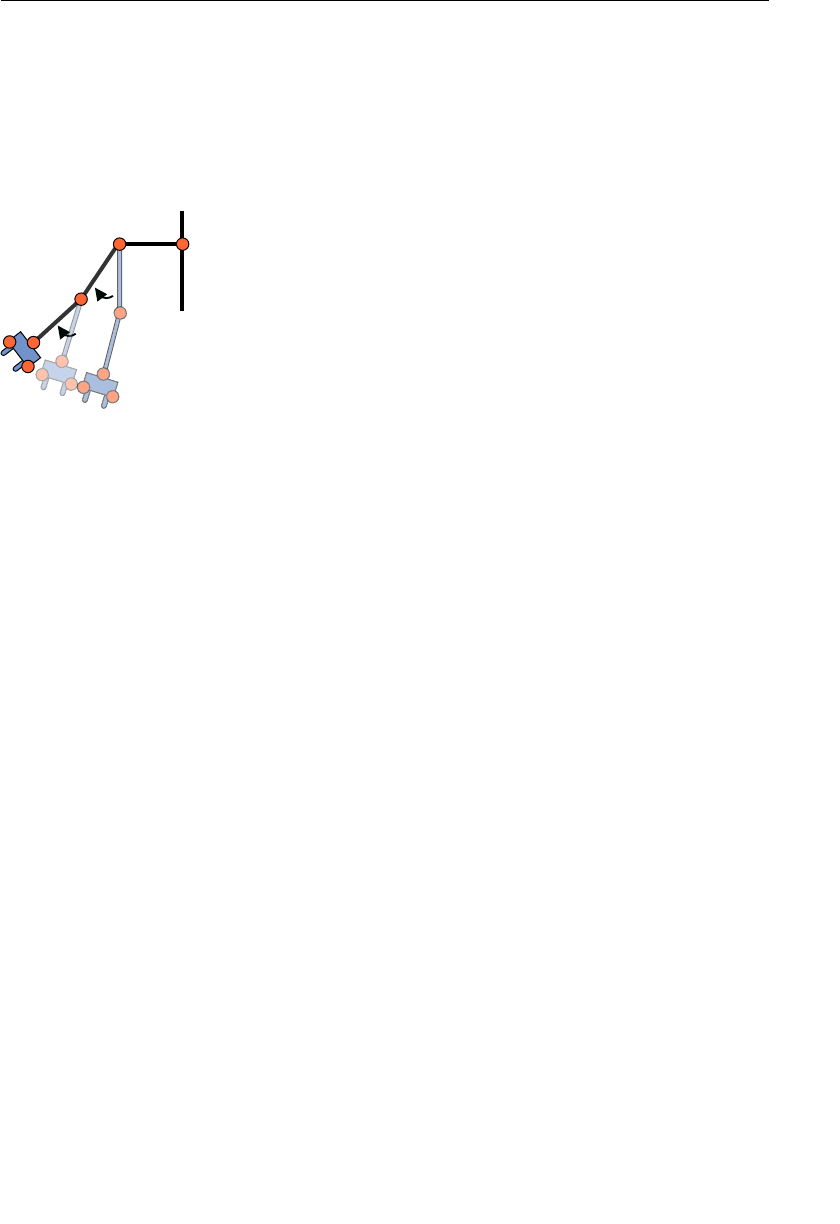
ptg11539634

CHAPTER 9 Hierarchical Objects

326

It is straightforward to program so that the rotation of one segment propagates to the

lower segments and simply requires that you use the same model matrix for the rotation

of the lower segments. For example, when you rotate a shoulder joint through 30 degrees

using one model matrix, you can draw the lower elbow and wrist joints rotated through

30 degrees using the same model matrix (see Figure 9.3 ). Thus, by changing only the angle

of the shoulder rotation, the lower segments are automatically rotated to follow the move-

ment of the shoulder joint.

30 degrees

rotate the shoulder joint

Figure 9.3 The lower segments following the rotation of the upper segment

For more complex cases, such as when you want to rotate the elbow joint 10 degrees after

rotating the shoulder joint 30 degrees, you can rotate the elbow joint by using the model

matrix and rotating 10 degrees more than the shoulder-joint model matrix. This can be

calculated by multiplying the shoulder-joint model matrix by a 10-degree rotation matrix,

which we refer to as the “elbow-joint model matrix.” The parts below the elbow will

follow the movement of the elbow when drawn using this elbow-joint model matrix.

By programming in such a way, the upper segments are not affected by rotation of the

lower segments. Thus, the upper segments will not move no matter how much the lower

segments move.

Now that you have a good understanding of the principles involved when moving multi-

segment objects, let’s look at a sample program.

Single Joint Model

Let’s begin with a simple single joint model. You will construct the program JointModel

that draws a robot arm consisting of two parts that can be manipulated with the arrow

keys. The screen shot and the hierarchy structure are shown on the left and right of Figure

9.4 , respectively. This robot arm consists of arm1 and arm2, which are joined by joint1.

You should imagine that the arm is raised above the shoulder and that arm1 is the upper

part and arm2 the lower part. When you add the hand later, it will become clearer.

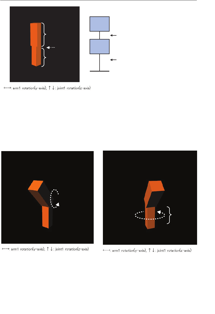
ptg11539634

Drawing and Manipulating Objects Composed of Other Objects 327

2mra

sixa—yehtdnuoragnitator

sixa—zehtdnuoragnitator

arm2

arm1

joint1 1mra

Figure 9.4 JointModel and the hierarchy structure used in the program

If you run the program, you will see that arm1 is rotated around the y-axis using the right

and left arrow keys, and joint1 is rotated around the z-axis with the up and down arrow

keys ( Figure 9.5 ). When pressing the down arrow key, joint1 is rotated and arm2 leans

forward, as shown on the left of Figure 9.5 . Then if you press the right arrow key, arm1 is

rotated, as shown on the right of Figure 9.5 .

arm2

Figure 9.5 The display change when pressing the arrow keys in JointModel

As you can see, the movement of arm2 by rotation of joint1 does not affect arm1. In

contrast, arm2 is rotated if you rotate arm1.

arm1

ptg11539634

CHAPTER 9 Hierarchical Objects

328

Sample Program (JointModel.js)

JointModel.js is shown in Listing 9.1 . The actual vertex shader is a little complicated

because of the shading process and has been removed from the listing here to save space.

However, if you are interested in how the lessons learned in the earlier part of the chapter

are applied, please look at the full listing available by downloading the examples from the

book website. The lighting used is a directional light source and simplified diffuse reflec-

tion, which makes the robot arm look more three-dimensional. However, as you can see,

there are no special lighting calculations needed for this joint model, and all the code

required to draw and manipulate the joint model is in the JavaScript program.

Listing 9.1 JointModel.js

1 // JointModel.js

2 // Vertex shader program

3 var VSHADER_SOURCE =

4 ‘attribute vec4 a_Position;n’ +

5 ‘attribute vec4 a_Normal;n’ +

6 ‘uniform mat4 u_MvpMatrix;n’ +

…

9 ‘void main() {n’ +

10 ‘ gl_Position = u_MvpMatrix * a_Position;n’ +

11 // Shading calculation to make the arm look three-dimensional

…

17 ‘}n’;

…

29 function main() {

…

46 // Set the vertex coordinate.

47 var n = initVertexBuffers(gl);

…

57 // Get the storage locations of uniform variables

58 var u_MvpMatrix = gl.getUniformLocation(gl.program, ‘u_MvpMatrix’);

59 var u_NormalMatrix = gl.getUniformLocation(gl.program, ‘u_NormalMatrix’);

…

65 // Calculate the view projection matrix

66 var viewProjMatrix = new Matrix4();

67 viewProjMatrix.setPerspective(50.0, canvas.width / canvas.height, 1.0, 100.0);

68 viewProjMatrix.lookAt(20.0, 10.0, 30.0, 0.0, 0.0, 0.0, 0.0, 1.0, 0.0);

70 // Register the event handler to be called when keys are pressed

71 document.onkeydown = function(ev){ keydown(ev, gl, n, viewProjMatrix,

➥u_MvpMatrix, u_NormalMatrix); };

72 // Draw robot arm

73 draw(gl, n, viewProjMatrix, u_MvpMatrix, u_NormalMatrix);

74 }

ptg11539634

Drawing and Manipulating Objects Composed of Other Objects 329

76 var ANGLE_STEP = 3.0; // The increments of rotation angle (degrees)

77 var g_arm1Angle = 90.0; // The rotation angle of arm1 (degrees)

78 var g_joint1Angle = 0.0; // The rotation angle of joint1 (degrees)

80 function keydown(ev, gl, n, viewProjMatrix, u_MvpMatrix, u_NormalMatrix) {

81 switch (ev.keyCode) {

82 case 38: // Up arrow key -> positive rotation of joint1 (z-axis)

83 if (g_joint1Angle < 135.0) g_joint1Angle += ANGLE_STEP;

84 break;

85 case 40: // Down arrow key -> negative rotation of joint1 (z-axis)

86 if (g_joint1Angle > -135.0) g_joint1Angle -= ANGLE_STEP;

87 break;

…

91 case 37: // Left arrow key -> negative rotation of arm1 (y-axis)

92 g_arm1Angle = (g_arm1Angle — ANGLE_STEP) % 360;

93 break;

94 default: return;

95 }

96 // Draw the robot arm

97 draw(gl, n, viewProjMatrix, u_MvpMatrix, u_NormalMatrix);

98 }

100 function initVertexBuffers(gl) {

101 // Vertex coordinates

…

148 }

…

174 // Coordinate transformation matrix

175 var g_modelMatrix = new Matrix4(), g_mvpMatrix = new Matrix4();

176

177 function draw(gl, n, viewProjMatrix, u_MvpMatrix, u_NormalMatrix) {

…

181 // Arm1

182 var arm1Length = 10.0; // Length of arm1

183 g_modelMatrix.setTranslate(0.0, -12.0, 0.0);

184 g_modelMatrix.rotate(g_arm1Angle, 0.0, 1.0, 0.0); // Rotate y-axis

185 drawBox(gl, n, viewProjMatrix, u_MvpMatrix, u_NormalMatrix); // Draw

186

187 // Arm2

188 g_modelMatrix.translate(0.0, arm1Length, 0.0); // Move to joint1

189 g_modelMatrix.rotate(g_joint1Angle, 0.0, 0.0, 1.0);// Rotate z-axis

190 g_modelMatrix.scale(1.3, 1.0, 1.3); // Make it a little thicker

191 drawBox(gl, n, viewProjMatrix, u_MvpMatrix, u_NormalMatrix); // Draw

192 }

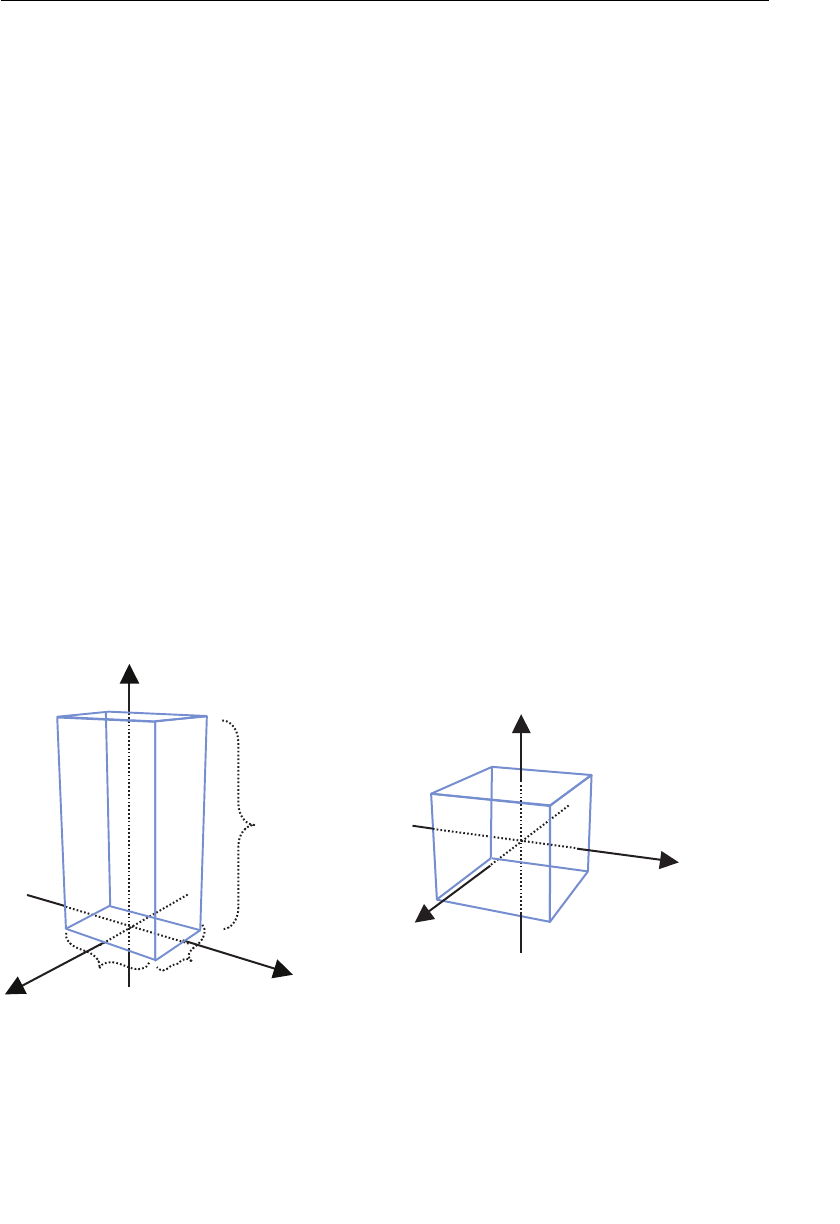
ptg11539634

CHAPTER 9 Hierarchical Objects

330

193

194 var g_normalMatrix = new Matrix4(); // Transformation matrix for normal

195

196 // Draw a cube

197 function drawBox(gl, n, viewProjMatrix, u_MvpMatrix, u_NormalMatrix) {

198 //Calculate the model view project matrix and pass it to u_MvpMatrix

199 g_mvpMatrix.set(viewProjMatrix);

200 g_mvpMatrix.multiply(g_modelMatrix);

201 gl.uniformMatrix4fv(u_MvpMatrix, false, g_mvpMatrix.elements);

202 // Calculate the normal transformation matrix and pass it to u_NormalMatrix

203 g_normalMatrix.setInverseOf(g_modelMatrix);

204 g_normalMatrix.transpose();

205 gl.uniformMatrix4fv(u_NormalMatrix, false, g_normalMatrix.elements);

206 // Draw

207 gl.drawElements(gl.TRIANGLES, n, gl.UNSIGNED_BYTE, 0);

208 }

The function main() from line 29 follows the same structure as before, with the first major

difference being the

initVertexBuffers() function call at line 47. In initVertexBuf-

fers() , the vertex data for arm1 and arm2 are written into the appropriate buffer objects.

Until now, you’ve been using cubes, with each side being 2.0 in length and the origin

at the center of the cube. Now, to better model the arm, you will use a cuboid like that

shown in the left side of Figure 9.6 . The cuboid has its origin at the center of the bottom

surface and is 3.0 by 3.0 and 10.0 units in height. By setting the origin at the center of the

bottom surface, its rotation around the z-axis is the same as that of joint1 in Figure 9.5 ,

making it convenient to program. Both arm1 and arm2 are drawn using this cuboid.

0.01

0.3

v6(-1, 1, -1)

v1(-1, 1, 1)

v7(-1, -1, -1)

v2(-1, -1, 1)

v3(1, -1, 1)

v4(1, -1, -1)

v0(1, 1, 1)

v5(1, 1, -1)

the previous cube

Figure 9.6 A cuboid for drawing the robot arm

ptg11539634

Drawing and Manipulating Objects Composed of Other Objects 331

From lines 66 to 68, a view projection matrix ( viewProjMatrix ) is calculated with the

specified viewing volume, the eye position, and the view direction.

Because the robot arm in this program is moved by using the arrow keys, the event

handler

keydown() is registered at line 71:

70 // Register the event handler to be called when keys are pressed

71 document.onkeydown = function(ev){ keydown(ev, gl, n, viewProjMatrix,

➥u_MvpMatrix, u_NormalMatrix); };

72 // Draw the robot arm

73 draw(gl, n, viewProjMatrix, u_MvpMatrix, u_NormalMatrix);

The keydown() function itself is defined at line 80. Before that, at lines 76, 77, and 78, the

definition of global variables used in

keydown() is defined:

76 var ANGLE_STEP = 3.0; // The increments of rotation angle (degrees)

77 var g_arm1Angle = -90.0; // The rotation angle of arm1 (degrees)

78 var g_joint1Angle = 0.0; // The rotation angle of joint1 (degrees)

80 function keydown(ev, gl, n, u_MvpMatrix, u_NormalMatrix) {

81 switch (ev.keyCode) {

82 case 38: // Up arrow key -> the positive rotation of joint1 (z-axis)

83 if (g_joint1Angle < 135.0) g_joint1Angle += ANGLE_STEP;

84 break;

…

88 case 39: // Right arrow key -> the positive rotation of arm1 (y-axis)

89 g_arm1Angle = (g_arm1Angle + ANGLE_STEP) % 360;

90 break;

…

95 }

96 // Draw the robot arm

97 draw(gl, n, u_MvpMatrix, u_NormalMatrix);

98 }

ANGLE_STEP at line 76 is used to control how many degrees arm1 and joint1 are rotated

each time the arrow keys are pressed and is set at 3.0 degrees.

g_arm1Angle (line 77) and

g_joint1Angle (line 78) are variables that store the current rotation angle of arm1 and

joint1, respectively (see Figure 9.7 ).

ptg11539634

CHAPTER 9 Hierarchical Objects

332

g_joint1Angle

g_arm1Angle

Figure 9.7 g_joint1Angle and g_arm1Angle

The

keydown() function , from line 80, increases or decreases the value of the rotation

angle of arm1 (

g_arm1Angle ) or joint1 ( g_joint1Angle ) by ANGLE_STEP , according to which

key is pressed. joint1 can only be rotated through the range from –135 degrees to 135

degrees so that arm2 does not interfere with arm1. Then the whole robot arm is drawn at

line 97 using the function

draw() .

Draw the Hierarchical Structure (draw())

The draw() function draws the robotic arm according to its hierarchical structure and is

defined at line 177. Two global variables,

g_modelMatrix and g_mvpMatrix , are created at

line 175 and will be used in both

draw() and drawBox() :

174 // Coordinate transformation matrix

175 var g_modelMatrix = new Matrix4(), g_mvpMatrix = new Matrix4();

176

177 function draw(gl, n, viewProjMatrix, u_MvpMatrix, u_NormalMatrix) {

…

181 // Arm1

182 var arm1Length = 10.0; // Length of arm1

183 g_modelMatrix.setTranslate(0.0, -12.0, 0.0);

184 g_modelMatrix.rotate(g_arm1Angle, 0.0, 1.0, 0.0); // Rotate y-axis

185 drawBox(gl, n, viewProjMatrix, u_MvpMatrix, u_NormalMatrix); // Draw

186

187 // Arm2

188 g_modelMatrix.translate(0.0, arm1Length, 0.0); // Move to joint1

189 g_modelMatrix.rotate(g_joint1Angle, 0.0, 0.0, 1.0); // Rotate z-axis

190 g_modelMatrix.scale(1.3, 1.0, 1.3); // Make it a little thicker

191 drawBox(gl, n, viewProjMatrix, u_MvpMatrix, u_NormalMatrix); // Draw

192 }

ptg11539634

Drawing and Manipulating Objects Composed of Other Objects 333

As you can see, draw() draws the segments by using drawBox() , starting with the upper

part (arm1) followed by the lower part (arm2).

When drawing each part, the same process is repeated: (1) translation (

setTranslate() ,

translate() ), (2) rotation ( rotate() ), and (3) drawing the part ( drawBox() ).

When drawing a hierarchical model performing a rotation, typically you will process from

upper to lower in the order of (1) translation, (2) rotation, and (3) drawing segments.

arm1 is translated to (0.0, –12.0, 0.0) with

setTranslate() at line 183 to move to an easily

visible position. Because this arm is rotated around the y-axis, its model matrix (

g_model-

Matrix ) is multiplied by the rotation matrix around the y-axis at line 184. g_arm1Angle

is used here. Once arm1’s coordinate transformation has been completed, you then draw

using the

drawBox() function.

Because arm2 is connected to the tip of arm1, as shown in Figure 9.7 , it has to be drawn

from the tip of arm1. This can be achieved by translating it along the y-axis in the posi-

tive direction by the length of arm1 (

arm1Length ) and applying the translation to the

model matrix, which is used when drawing arm1 (

g_modelMatrix ).

This is done as shown in line 188, where the second argument of translate() is

arm1Length . Also notice that the method uses translate() rather than setTranslate()

because arm2 is drawn at the tip of arm1:

187 // Arm2

188 g_modelMatrix.translate(0.0, arm1Length, 0.0); // Move to joint1

189 g_modelMatrix.rotate(g_joint1Angle, 0.0, 0.0, 1.0); // Rotate z-axis

190 g_modelMatrix.scale(1.3, 1.0, 1.3); // Make it a little thicker

191 drawBox(gl, n, viewProjMatrix, u_MvpMatrix, u_NormalMatrix); // Draw

Line 189 handles the rotation of arm2 which, as can be seen, uses g_joint1Angle . You

make arm2 a little thicker at line 190 by scaling it along the x and z direction. This makes

it easier to distinguish between the two arm segments but is not essential to the robotic

arm’s movement.

Now, by updating

g_arm1Angle and g_joint1Angle in keydown() as described in the previ-

ous section and then invoking

draw() , arm1 is rotated by g_arm1Angle and arm2 is, in

addition, rotated by

g_joint1Angle .

The drawBox() function is quite simple. It calculates a model view project matrix and

passes it to the

u_MvpMatrix variable at lines 199 and 200. Then it just calculates the

normal transformation matrix for shading from the model matrix, sets it to

u_NormalMatrix at lines 203 and 204, and draws the cuboid in Figure 9.6 at line 207.

This basic approach, although used here for only a single joint, can be used for any

complex hierarchical models simply by repeating the process steps used earlier.

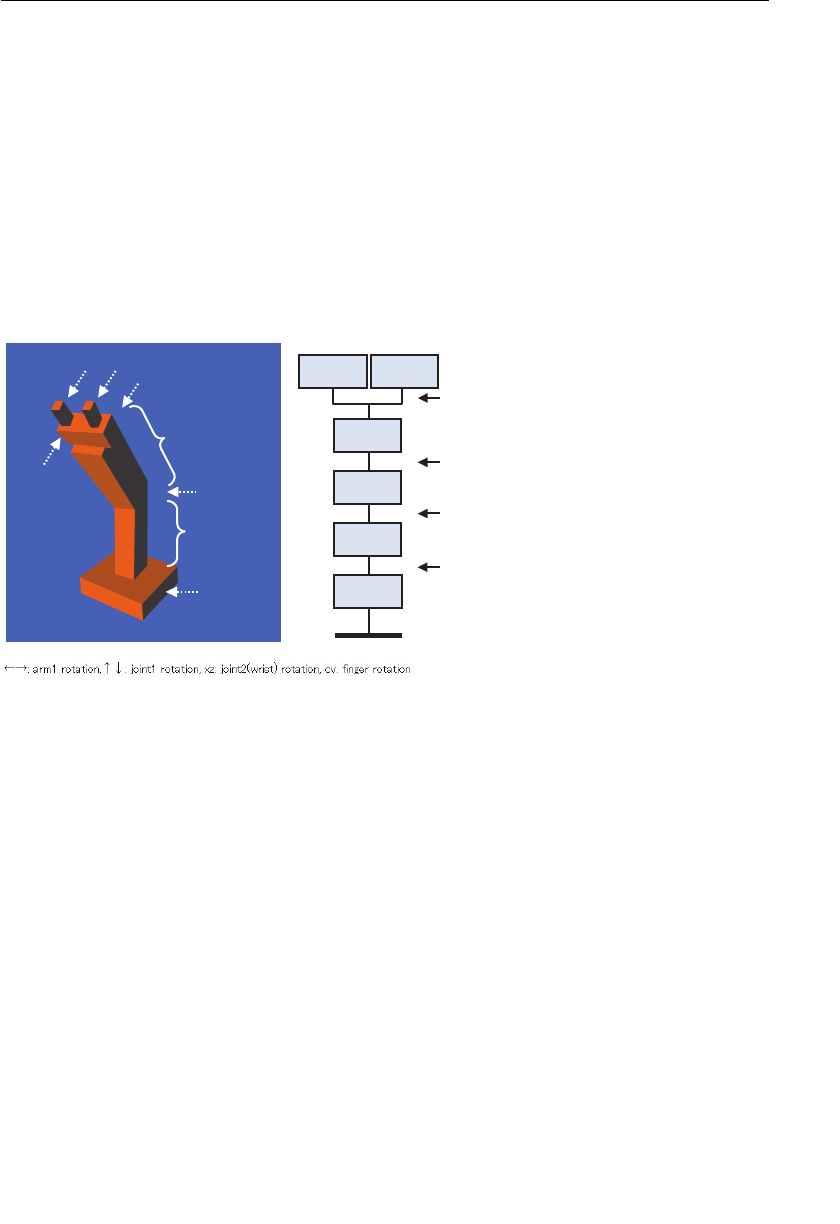
ptg11539634

CHAPTER 9 Hierarchical Objects

334

Obviously, our simple robot arm, although modeled on a human arm, is more like a

skeleton than a real arm. A more realistic model of a real arm would require the skin to

be modeled, which is beyond the scope of this book. Please refer to the OpenGL ES 2.0

Programming Guide for more information about skinning.

A Multijoint Model

Here, you will extend JointModel to create MultiJointModel , which draws a multijoint

robot arm consisting of two arm segments, a palm, and two fingers, all of which you can

manipulate using the keyboard. As shown in Figure 9.8 , we call the arm extending from

the base arm1, the next segment arm2, and the joint between the two arms joint1. There

is a palm at the tip of arm2. The joint between arm2 and the palm is called joint2. The

two fingers attached at the end of the palm are respectively finger1 and finger2.

sixa—yehtdnuoraetator

sixa—xehtdnuoraetator

sixa—zehtdnuoraetator

sixa—yehtdnuoraetator

1mra

2mra

mlap

esab

arm1

base

palm

finger1 finger2

arm2

joint1

joint2 finger1 finger2

Figure 9.8 The hierarchical structure of MultiJointModel

Manipulation of arm1 and joint1 using the arrow keys is the same as

JointModel . In addi-

tion, you can rotate joint2 (wrist) with the X and Z keys and move (rotate) the two fingers

with the C and V keys. The variables controlling the rotation angle of each part are shown

in Figure 9.9 .

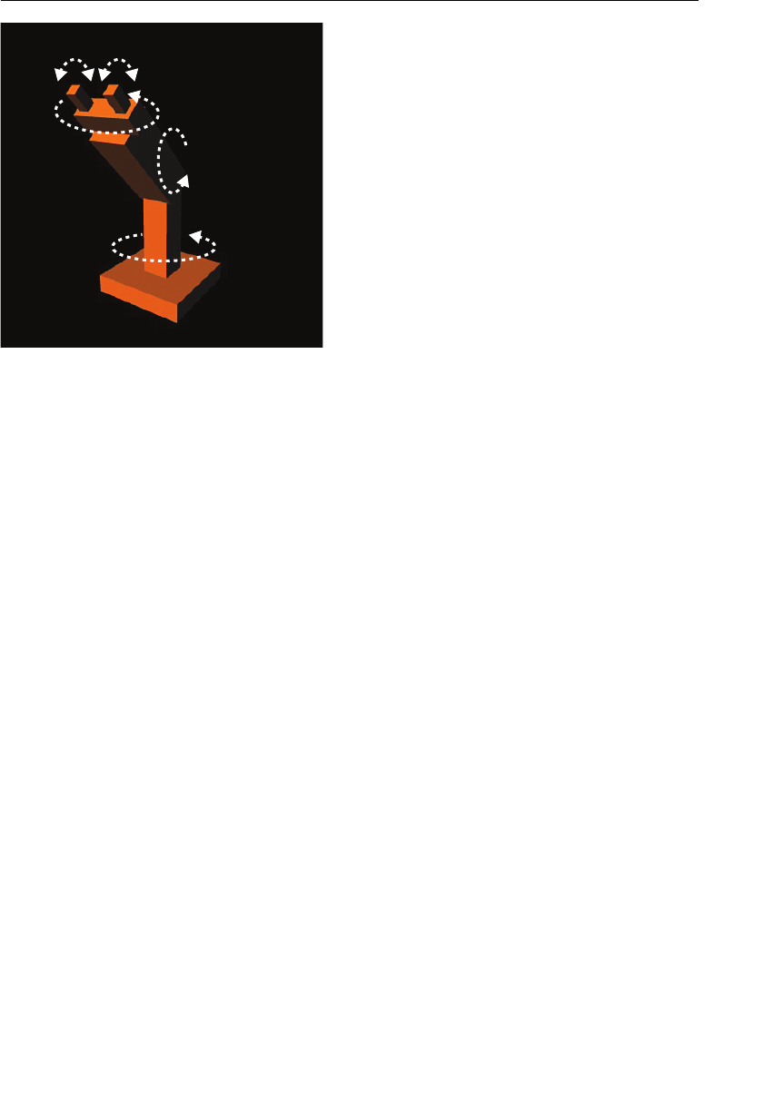
ptg11539634

Drawing and Manipulating Objects Composed of Other Objects 335

g_joint3Angle

g_joint2Angle

g_joint1Angle

g_arm1Angle

Figure 9.9 The variables controlling the rotation of segments

Sample Program (MultiJointModel.js)

This program is similar to JointModel , except for extensions to keydown() to handle the

additional control keys, and

draw() , which draws the extended hierarchical structure. First

let’s look at

keydown() in Listing 9.2 .

Listing 9.2 MultiJointModel.js (Code for Key Processing)

1 // MultiJointModel.js

…

76 var ANGLE_STEP = 3.0; // The increments of rotation angle (degrees)

77 var g_arm1Angle = 90.0; // The rotation angle of arm1 (degrees)

78 var g_joint1Angle = 45.0; // The rotation angle of joint1 (degrees)

79 var g_joint2Angle = 0.0; // The rotation angle of joint2 (degrees)

80 var g_joint3Angle = 0.0; // The rotation angle of joint3 (degrees)

82 function keydown(ev, gl, n, viewProjMatrix, u_MvpMatrix, u_NormalMatrix) {

83 switch (ev.keyCode) {

84 case 40: // Up arrow key -> positive rotation of joint1 (z-axis)

…

95 break;

96 case 90: // Z key -> the positive rotation of joint2

97 g_joint2Angle = (g_joint2Angle + ANGLE_STEP) % 360;

98 break;

99 case 88: // X key -> the negative rotation of joint2

100 g_joint2Angle = (g_joint2Angle — ANGLE_STEP) % 360;

101 break;

ptg11539634

CHAPTER 9 Hierarchical Objects

336

102 case 86: // V key -> the positive rotation of joint3

103 if (g_joint3Angle < 60.0) g_joint3Angle = (g_joint3Angle +

➥ANGLE_STEP) % 360;

104 break;

105 case 67: // C key -> the negative rotation of joint3

106 if (g_joint3Angle > -60.0) g_joint3Angle = (g_joint3Angle –

➥ANGLE_STEP) % 360;

107 break;

108 default: return;

109 }

110 // Draw the robot arm

111 draw(gl, n, viewProjMatrix, u_MvpMatrix, u_NormalMatrix);

112 }

keydown() is basically the same as that of JointAngle , but in addition to changing

g_arm1Angle and g_joint1Angle based on key presses, it processes the Z, X, V, and C

keys at lines 96, 99, 102, and 105. These key presses change

g_joint2Angle , which is the

rotation angle of joint2, and

g_joint3Angle , which is the rotation angle of joint3, respec-

tively. After changing them, it calls

draw() at line 111 to draw the hierarchy structure.

Let’s take a look at

draw() in Listing 9.3 .

Although you are using the same cuboid for the base, arm1, arm2, palm, finger1, and

finger2, the segments are different in width, height, and depth. To make it easy to draw

these segments, let’s extend

drawBox() with three more arguments than that used in the

single-joint model:

function drawBox(gl, n, width, height, depth , viewProjMatrix,

u_MvpMatrix

➥u_NormalMatrix)

By specifying the width, height, and depth using the third to fifth argument, this function

draws a cuboid of the specified size with its origin at the center of the bottom surface.

Listing 9.3 MultiJointModel.js (Code for Drawing the Hierarchy Structure)

188 // Coordinate transformation matrix

189 var g_modelMatrix = new Matrix4(), g_mvpMatrix = new Matrix4();

190

191 function draw(gl, n, viewProjMatrix, u_MvpMatrix, u_NormalMatrix) {

192 // Clear color buffer and depth buffer

193 gl.clear(gl.COLOR_BUFFER_BIT | gl.DEPTH_BUFFER_BIT);

194

195 // Draw a base

196 var baseHeight = 2.0;

197 g_modelMatrix.setTranslate(0.0, -12.0, 0.0);

198 drawBox(gl, n, 10.0, baseHeight, 10.0, viewProjMatrix, u_MvpMatrix,

➥u_NormalMatrix);

ptg11539634

Drawing and Manipulating Objects Composed of Other Objects 337

199

200 // Arm1

201 var arm1Length = 10.0;

202 g_modelMatrix.translate(0.0, baseHeight, 0.0); // Move onto the base

203 g_modelMatrix.rotate(g_arm1Angle, 0.0, 1.0, 0.0); // Rotation

204 drawBox(gl, n, 3.0, arm1Length, 3.0, viewProjMatrix, u_MvpMatrix,

➥u_NormalMatrix); // Draw

295

206 // Arm2

…

212 // A palm

213 var palmLength = 2.0;

…

218 // Move to the center of the tip of the palm

219 g_modelMatrix.translate(0.0, palmLength, 0.0);

220

221 // Draw finger1

222 pushMatrix(g_modelMatrix);

223 g_modelMatrix.translate(0.0, 0.0, 2.0);

224 g_modelMatrix.rotate(g_joint3Angle, 1.0, 0.0, 0.0); // Rotation

225 drawBox(gl, n, 1.0, 2.0, 1.0, viewProjMatrix, u_MvpMatrix, u_NormalMatrix);

226 g_modelMatrix = popMatrix();

227

228 // Draw finger2

229 g_modelMatrix.translate(0.0, 0.0, -2.0);

230 g_modelMatrix.rotate(-g_joint3Angle, 1.0, 0.0, 0.0); // Rotation

231 drawBox(gl, n, 1.0, 2.0, 1.0, viewProjMatrix, u_MvpMatrix, u_NormalMatrix);

232 }

233

234 var g_matrixStack = []; // Array for storing a matrix

235 function pushMatrix(m) { // Store the specified matrix to the array

236 var m2 = new Matrix4(m);

237 g_matrixStack.push(m2);

238 }

239

240 function popMatrix() { // Retrieve the matrix from the array

241 return g_matrixStack.pop();

242 }

The draw() function operates in the same way as in JointModel ; that is, each part

is handled following the order of (1) translation, (2) rotation, and (3) draw (using

drawBox() ). First, because the base is not rotated, after moving to the appropriate posi-

tion at line 197, it draws a base there with

drawBox() . The third to fifth arguments of

drawBox() specify a width of 10, height of 2, and depth of 10, which cause a flat stand to

be drawn.

ptg11539634

CHAPTER 9 Hierarchical Objects

338

The arm1, arm2, and palm are each drawn following the same order of (1) translation,

(2) rotation, and (3) draw and by moving down the object hierarchy toward the lower

level in the same manner as

JointModel .

The main difference in this sample program is the drawing of finger1 and finger2 from

line 222. Because they do not have a parent-child relationship, a little more care is needed.

In particular, you have to pay attention to the contents of the model matrix. First, let’s

look at finger1, whose position is translated 2.0 along the z-axis direction from the center

of the tip of the palm and rotated around the x-axis. finger1 can be drawn in the order of

(1) translating, (2) rotating, and (3) drawing segments as before. The program is as follows:

g_modelMatrix.translate(0.0, 0.0, 2.0);

g_modelMatrix.rotate(g_joint3Angle, 1.0, 0.0, 0.0); // Rotation

drawBox(gl, n, 1.0, 2.0, 1.0, u_MvpMatrix, u_NormalMatrix);

Next, looking at finger2, if you follow the same procedure a problem occurs. finger2’s

intended position is a translation of –2.0 units along the z-axis direction from the center

of the tip of the palm and rotated around the x-axis. However, because the model matrix

has changed, if you draw finger2, it will be drawn at the tip of finger1.

Clearly, the solution is to restore the model matrix to its state before finger1 was drawn. A

simple way to achieve this is to store the model matrix before drawing finger1 and retriev-

ing it after drawing finger1. This is actually done at lines 222 and 226 and uses the func-

tions

pushMatrix() and popMatrix() to store the specified matrix and retrieve it. At line

222, you store the model matrix specified as

pushMatrix() ’s argument ( g_modelMatrix ).

Then, after drawing finger1 at lines 223 to 225, you retrieve the old model matrix at line

226, with

popMatrix() , and assign it to g_modelMatrix . Now, because the model matrix

has reverted back, you can draw finger2 in the same way as before.

pushMatrix() and popMatrix() are shown next. pushMatrix() stores the matrix specified

as its argument in an array named

g_matrixStack at line 234. popMatrix() retrieves the

matrix stored in

g_matrixStack and returns it:

234 var g_matrixStack = []; // Array for storing matrices

235 function pushMatrix(m) { // Store the specified matrix

236 var m2 = new Matrix4(m);

237 g_matrixStack.push(m2);

238 }

239

240 function popMatrix() { // Retrieve a matrix from the array

241 return g_matrixStack.pop();

242 }

This approach can be used to draw an arbitrarily long robot arm. It will scale when new

segments are added to the hierarchy. You only need to use

pushMatrix() and popMatrix()

when the hierarchy structure is a sibling relation, not a parent-child relation.

ptg11539634

Drawing and Manipulating Objects Composed of Other Objects 339

Draw Segments (drawBox())

Finally, let’s take a look at drawBox() , which draws the segments of the robot arm using

the following arguments:

247 function drawBox(gl, n, width, height, depth, viewMatrix, u_MvpMatrix,

➥u_NormalMatrix) {

The third to fifth arguments, width , height, and depth , specify the width, height, and depth

of the cuboid being drawn. As for the remaining argument, viewMatrix is a view matrix,

and u_MvpMatrix and u_NormalMatrix are the arguments for setting the coordinate trans-

formation matrices to the corresponding uniform variables in the vertex shader, just like

JointModel.js . The model view projection matrix is passed to u_MvpMatrix , and the

matrix for transforming the coordinates of the normal, described in the previous section,

is passed to u_NormalMatrix .

The three-dimensional object used here, unlike JointModel, is a cube whose side is 1.0

unit long. Its origin is located at the center of the bottom surface so that you can easily

rotate the arms, the palm, and the fingers. The function

drawBox() is shown here:

244 var g_normalMatrix = new Matrix4();// Transformation matrix for normal

245

246 // Draw a cuboid

247 function drawBox(gl, n, width, height, depth, viewProjMatrix,

➥u_MvpMatrix, u_NormalMatrix) {

248 pushMatrix(g_modelMatrix); // Save the model matrix

249 // Scale a cube and draw

250 g_modelMatrix.scale(width, height, depth);

251 // Calculate model view project matrix and pass it to u_MvpMatrix

252 g_mvpMatrix.set(viewProjMatrix);

253 g_mvpMatrix.multiply(g_modelMatrix);

254 gl.uniformMatrix4fv(u_MvpMatrix, false, g_mvpMatrix.elements);

255 // Calculate transformation matrix for normals and pass it to u_NormalMatrix

…

259 // Draw

260 gl.drawElements(gl.TRIANGLES, n, gl.UNSIGNED_BYTE, 0);

261 g_modelMatrix = popMatrix(); // Retrieve the model matrix

262 }

As you can see, the model matrix is multiplied by a scaling matrix at line 250 so that

the cube will be drawn with the size specified by width , height, and depth . Note that you

store the model matrix at line 248 and retrieve it at line 261 using

pushMatrix() and

popMatrix() . Otherwise, when you draw arm2 after arm1, the scaling used for arm1 is left

in the model matrix and affects the drawing of arm2. By retrieving the model matrix at

line 261, which is saved at line 248, the model matrix reverts to the state before scaling

was applied at line 250.

ptg11539634

CHAPTER 9 Hierarchical Objects

340

As you can see, the use of pushMatrix() and popMatrix() adds an extra degree of

complexity but allows you to specify only one set of vertex coordinates and use scaling

to create different cuboids. The alternative approach, using multiple objects specified by

different sets of vertices, is also possible. Let’s take a look at how you would program that.

Draw Segments (drawSegment())

In this section, we will explain how to draw segments by switching between buffer objects

in which the vertex coordinates representing the shape of each segment are stored.

Normally, you would need to specify the vertex coordinates, the normal, and the indices

for each segment. However, in this example, because all segments are cuboids, you can

share the normals and indices and simply specify the vertices for each segment. For each

segment (the base, arm1, arm2, palm, and fingers), the vertices are stored in their respec-

tive object buffers, which are then switched when drawing the arm parts. Listing 9.4

shows the sample program.

Listing 9.4 MultiJointModel_segment.js

1 // MultiJointModel_segment.js

…

29 function main() {

…

47 var n = initVertexBuffers(gl);

…

57 // Get the storage locations of attribute and uniform variables

58 var a_Position = gl.getAttribLocation(gl.program, ‘a_Position’);

…

74 draw(gl, n, viewProjMatrix, a_Position, u_MvpMatrix, u_NormalMatrix);

75 }

…

115 var g_baseBuffer = null; // Buffer object for a base

116 var g_arm1Buffer = null; // Buffer object for arm1

117 var g_arm2Buffer = null; // Buffer object for arm2

118 var g_palmBuffer = null; // Buffer object for a palm

119 var g_fingerBuffer = null; // Buffer object for fingers

120

121 function initVertexBuffers(gl){

122 // Vertex coordinate (Coordinates of cuboids for all segments)

123 var vertices_base = new Float32Array([ // Base(10x2x10)

124 5.0, 2.0, 5.0, -5.0, 2.0, 5.0, -5.0, 0.0, 5.0, 5.0, 0.0, 5.0,

125 5.0, 2.0, 5.0, 5.0, 0.0, 5.0, 5.0, 0.0,-5.0, 5.0, 2.0,-5.0,

…

129 5.0, 0.0,-5.0, -5.0, 0.0,-5.0, -5.0, 2.0,-5.0, 5.0, 2.0,-5.0

130 ]);

131

ptg11539634

Drawing and Manipulating Objects Composed of Other Objects 341

132 var vertices_arm1 = new Float32Array([ // Arm1(3x10x3)

133 1.5, 10.0, 1.5, -1.5, 10.0, 1.5, -1.5, 0.0, 1.5, 1.5, 0.0, 1.5,

134 1.5, 10.0, 1.5, 1.5, 0.0, 1.5, 1.5, 0.0,-1.5, 1.5, 10.0,-1.5,

…

138 1.5, 0.0,-1.5, -1.5, 0.0,-1.5, -1.5, 10.0,-1.5, 1.5, 10.0,-1.5

139 ]);

…

159 var vertices_finger = new Float32Array([ // Fingers(1x2x1)

…

166 ]);

167

168 // normals

169 var normals = new Float32Array([

…

176 ]);

177

178 // Indices of vertices

179 var indices = new Uint8Array([

180 0, 1, 2, 0, 2, 3, // front

181 4, 5, 6, 4, 6, 7, // right

…

185 20,21,22, 20,22,23 // back

186 ]);

187

188 // Write coords to buffers, but don’t assign to attribute variables

189 g_baseBuffer = initArrayBufferForLaterUse(gl, vertices_base, 3, gl.FLOAT);

190 g_arm1Buffer = initArrayBufferForLaterUse(gl, vertices_arm1, 3, gl.FLOAT);

…

193 g_fingerBuffer = initArrayBufferForLaterUse(gl, vertices_finger, 3, gl.FLOAT);

…

196 // Write normals to a buffer, assign it to a_Normal, and enable it

197 if (!initArrayBuffer(gl, ‘a_Normal’, normals, 3, gl.FLOAT)) return null;

198

199 // Write indices to a buffer

200 var indexBuffer = gl.createBuffer();

…

205 gl.bindBuffer(gl.ELEMENT_ARRAY_BUFFER, indexBuffer);

206 gl.bufferData(gl.ELEMENT_ARRAY_BUFFER, indices, gl.STATIC_DRAW);

207

208 return indices.length;

209 }

…

255 function draw(gl, n, viewProjMatrix, a_Position, u_MvpMatrix, u_NormalMatrix) {

…

ptg11539634

CHAPTER 9 Hierarchical Objects

342

259 // Draw a base

260 var baseHeight = 2.0;

261 g_modelMatrix.setTranslate(0.0, -12.0, 0.0);

262 drawSegment(gl, n, g_baseBuffer, viewProjMatrix, a_Position,

➥u_MvpMatrix, u_NormalMatrix);

263

264 // Arm1

265 var arm1Length = 10.0;

266 g_modelMatrix.translate(0.0, baseHeight, 0.0); // Move to the tip of the base

267 g_modelMatrix.rotate(g_arm1Angle, 0.0, 1.0, 0.0); // Rotate y-axis

268 drawSegment(gl, n, g_arm1Buffer, viewProjMatrix, a_Position,

➥u_MvpMatrix, u_NormalMatrix);

269

270 // Arm2

…

292 // Finger2

…

295 drawSegment(gl, n, g_fingerBuffer, viewProjMatrix, a_Position,

➥u_MvpMatrix, u_NormalMatrix);

296 }

…

310 // Draw segments

311 function drawSegment(gl, n, buffer, viewProjMatrix, a_Position,

➥u_MvpMatrix, u_NormalMatrix) {

312 gl.bindBuffer(gl.ARRAY_BUFFER, buffer);

313 // Assign the buffer object to the attribute variable

314 gl.vertexAttribPointer(a_Position, buffer.num, buffer.type, false, 0, 0);

315 // Enable the assignment

316 gl.enableVertexAttribArray(a_Position);

317

318 // Calculate the model view project matrix and set it to u_MvpMatrix

…

322 // Calculate matrix for normal and pass it to u_NormalMatrix

…

327 gl.drawElements(gl.TRIANGLES, n, gl.UNSIGNED_BYTE, 0);

328 }

The key points in this program are (1) creating the separate buffer objects that contain the

vertex coordinates for each segment, (2) before drawing each segment, assigning the corre-

sponding buffer object to the attribute variable

a_Position , and (3) enabling the buffer

and then drawing the segment.

The

main() function from line 29 in the JavaScript code follows the same steps as before.

Switching between buffers for the different segments is added to

initVertexBuffers() ,

ptg11539634

Drawing and Manipulating Objects Composed of Other Objects 343

called at line 47. The stored location of a_Position is retrieved at line 58, and then draw()

is called at line 73.

Let’s examine

initVertex() , defined at line 121. Lines 115 to 119 declare the buffer

objects as global variables, used to store the vertex coordinates of each segment. Within

the function, one of the main differences from

MultiJointModel.js is the definition of

the vertex coordinates from line 123. Because you are not using a single cuboid trans-

formed differently for the different segments, you need to define the vertex coordinates

for all the parts separately (for example, the base (

vertices_base ) at line 123, coordinates

for arm1 (

vertices_arm1 ), at line 132. The actual creation of the buffer objects for each

part occurs in the function

initArrayBufferForLaterUse() from line 189 to 193. This

function is shown here:

211 function initArrayBufferForLaterUse(gl, data, num, type){

212 var buffer = gl.createBuffer(); // Create a buffer object

…

217 // Write data to the buffer object

218 gl.bindBuffer(gl.ARRAY_BUFFER, buffer);

219 gl.bufferData(gl.ARRAY_BUFFER, data, gl.STATIC_DRAW);

220

221 // Store information to assign it to attribute variable later

222 buffer.num = num;

223 buffer.type = type;

224

225 return buffer;

226 }

initArrayBufferForLaterUse() simply creates a buffer object at line 212 and writes data

to it at lines 218 and 219. Notice that assigning it to an attribute variable (

gl.vertex

AttribPointer() ) and enabling the assignment ( gl.enableVertexAttribAray() ) are not

done within the function but later, just before drawing. To assign the buffer object to the

attribute variable

a_Position later, the data needed is stored as properties of the buffer

object at lines 222 and 223.

Here you take advantage of an interesting feature of JavaScript that allows you to freely

add new properties of an object and assign data to them. You can do this by simply

appending the

.property-name to the object name and assigning a value. Using this

feature, you store the number of items in the

num property (line 222), and the type in the

type property (line 223). Of course, you can access the contents of the newly made prop-

erties using the same name. Note, you must be careful when referring to properties created

in this way, because JavaScript gives no error indications even if you misspell only one

character in the property name. Equally, be aware that, although convenient, appending

properties has a performance overhead. A better approach, user-defined types, is explained

in Chapter 10 , “Advanced Techniques,” but let’s stick with this approach for now.

ptg11539634

CHAPTER 9 Hierarchical Objects

344

Finally, the draw() function, invoked at line 255, is the same as used in MultiJointModel

in terms of drawing parts according to the hierarchical structure, but it’s different in

terms of using

drawSegment() to draw each segment. In particular, the third argument of

drawSegment() , shown next, is the buffer object in which the vertex coordinates of the

parts are stored.

262 drawSegment(gl, n, g_baseBuffer, viewProjMatrix, u_MvpMatrix, u_NormalMatrix);

This function is defined at line 311 and operates as follows. It assigns a buffer object to

the attribute variable

a_Position and enables it at lines 312 to 316 before drawing at line

327. Here,

num and type , which are just stored as buffer object properties, are used.

310 // Draw segments

311 function drawSegment(gl, n, buffer, viewProjMatrix, a_Position,

➥u_MvpMatrix, u_NormalMatrix) {

312 gl.bindBuffer(gl.ARRAY_BUFFER, buffer);

313 // Assign the buffer object to the attribute variable

314 gl.vertexAttribPointer(a_Position, buffer.num, buffer.type, false, 0, 0);

315 // Enable the assignment

316 gl.enableVertexAttribArray(a_Position);

317

318 // Calculate model view project matrix and set it to u_MvpMatrix

…

322 // Calculate transformation matrix for normal and set it to u_NormalMatrix

…

327 gl.drawElements(gl.TRIANGLES, n, gl.UNSIGNED_BYTE, 0);

328 }

This time you don’t need to scale objects with the model matrix because you have

prepared the vertex coordinates per part, so there is no need to store and retrieve the

matrix. Therefore,

pushMatrix() and popMatrix() are not necessary.

Shader and Program Objects: The Role of

initShaders()

Finally, before we wrap up this chapter, let’s examine one of the convenience functions

defined for this book:

initShaders() . This function has been used in all the sample

programs and has hidden quite a lot of complex detail about setting up and using shaders.

We have deliberately left this explanation to the end of this chapter to ensure you have a

good understanding of the basics of WebGL before tackling some of these complex details.

We should note that it’s not actually necessary to master these details. For some readers

it will be sufficient to simply reuse the

initShaders() function we supply and skip this

section. However, for those who are interested, let’s take a look.

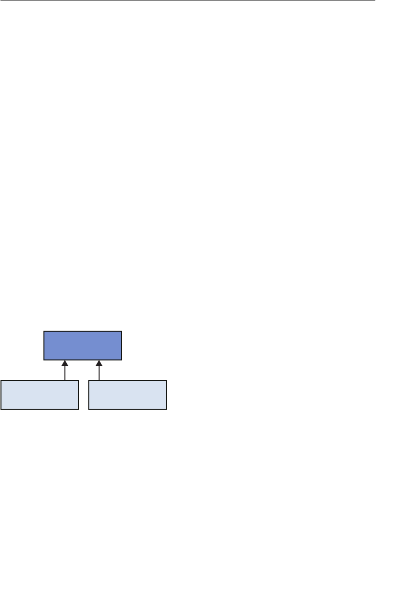
ptg11539634

Shader and Program Objects: The Role of initShaders() 345

initShaders() carries out the routine work to make shaders available in WebGL. It

consists of seven steps:

1. Create shader objects (

gl.createShader() ).

2. Store the shader programs (to avoid confusion, we refer to them as “source code”) in

the shader objects (

g.shaderSource() ).

3. Compile the shader objects ( gl.compileShader() ).

4. Create a program object ( gl.createProgram() ).

5. Attach the shader objects to the program object ( gl.attachShader() ).

6. Link the program object (

gl.linkProgram() ).

7. Tell the WebGL system the program object to be used (

gl.useProgram() ).

Each step is simple but when combined can appear complex, so let’s take a look at them

one by one. First, as you know from earlier, two types of objects are necessary to use

shaders: shader objects and program objects.

Shader object A shader object manages a vertex shader or a fragment shader. One

shader object is created per shader.

Program object A program object is a container that manages the shader objects. A vertex

shader object and a fragment shader object (two shader objects in total)

must be attached to a program object in WebGL.

The relationship between a program object and shader objects is shown in Figure 9.10 .

A program object

shader object

(vertex shader)

shader object

(fragment shader)

Figure 9.10 The relationship between a program object and shader objects

Using this information, let’s discuss the preceding seven steps sequentially.

Create Shader Objects (gl.createShader())

All shader objects have to be created with a call to gl.createShader() before using them.

ptg11539634

CHAPTER 9 Hierarchical Objects

346

gl.createShader(type)

Create a shader of the specified type .

Parameters type Specifies the type of shader object to be created: either

gl.VERTEX_SHADER (a vertex shader) or gl.FRAGMENT_

SHADER (a fragment shader).

Return value Non-null The created shader object.

null The creation of the shader object failed.

Errors INVALID_ENUM The specified type is none of the above.

gl.createShader() creates a vertex shader or a fragment shader according to the specified

type . If you do not need the shader any more, you can delete it with

gl.deleteShader() .

gl.deleteShader(shader)

Delete the shader object.

Parameters shader Specifies the shader object to be deleted.

Return value None

Errors None

Note that the specified shader object is not deleted immediately if it is still in use (that is,

it is attached to a program object using

gl.attachShader() , which is discussed in a few

pages). The shader object specified as an argument of

gl.deleteShader() will be deleted

when a program object no longer uses it.

Store the Shader Source Code in the Shader Objects

(g.shaderSource())

A shader object has storage to store the shader source code (written as a string in the

JavaScript program or in the separate file; see Appendix F , “Loading Shader Programs from

Files”). You use

gl.shaderSource() to store the source code in a shader object.

ptg11539634

Shader and Program Objects: The Role of initShaders() 347

gl.shaderSource(shader, source)

Store the source code specified by source in the shader object specified by shader . If any

source code was previously stored in the shader object, it is replaced by new source code.

Parameters shader Specifies the shader object in which the program is stored.

source Specifies the shader source code (string)

Return value None

Errors None

Compile Shader Objects (gl.compileShader())

After storing the shader source code in the shader object, you have to compile it so that

it can be used in the WebGL system. Unlike JavaScript, and like C or C++, shaders need

to be compiled before use. In this process, the source code stored in a shader object is

compiled to executable format (binary) and kept in the WebGL system. Use

gl.compile-

Shader() to compile. Note, if you replace the source code in the shader object with a call

gl.shaderSource() after compiling, the compiled binary kept in the shader object is

not replaced. You have to recompile it explicitly.

gl.compileShader(shader)

Compile the source code stored in the shader object specified by shader .

Parameters shader Specifies the shader object in which the source code to be

compiled is stored.

Return Value None

Errors None

When executing

gl.compileShader() , it is possible a compilation error occurs due to

mistakes in the source code. You can check for such errors, as well as the status of the

shader object, using

gl.getShaderParameter() .

ptg11539634

CHAPTER 9 Hierarchical Objects

348

gl.getShaderParameter(shader, pname)

Get the information specified by pname from the shader object specified by shader .

Parameters shader Specifies the shader object.

pname Specifies the information to get from the shader:

gl.SHADER_TYPE , gl.DELETE_STATUS , or

gl.COMPILE_STATUS .

Return value The following depending on pname :

gl.SHADER_TYPE The type of shader ( gl.VERTEX_SHADER or gl.FRAGMENT_

SHADER )

gl.DELETE_

STATUS

Whether the deletion has succeeded (

true or false )

gl.COMPILE_

STATUS

Whether the compilation has succeeded (

true or false )

Errors INVALID_ENUM pname is none of the above values.

To check whether the compilation succeeded, you can call

gl.getShaderParameter() with

gl.COMPILE_STATUS specified in pname .

If the compilation has failed, gl.getShaderParameter() returns false , and the error infor-

mation is written in the information log for the shader in the WebGL system. This infor-

mation can be retrieved with

gl.getShaderInfoLog() .

gl.getShaderInfoLog(shader)

Retrieve the information log from the shader object specified by shader .

Parameters shader Specifies the shader object from which the information log is

retrieved.

Return value non-null The string containing the logged information .

null Any errors are generated.

Errors None

Although the exact details of the logged information is implementation specific, almost

all WebGL systems return error messages containing the line numbers where the compiler

ptg11539634

Shader and Program Objects: The Role of initShaders() 349

has detected the errors in the program. For example, assume that you compiled a fragment

shader program as follows:

var FSHADER_SOURCE =

‘void main() {n’ +

‘ gl.FragColor = vec4(1.0, 0.0, 0.0, 1.0);n’ +

‘}n’;

Because the second line is incorrect in this case ( gl. must be gl_ ), the error messages

displayed in the JavaScript console of Chrome will be similar to those shown in Figure 9.11 .

Figure 9.11 A compile error in a shader

The first message indicates that

gl at line 2 is undeclared.

failed to compile shader: ERROR: 0: 2 : ‘gl’ : undeclared identifier

cuon-utils.js:88

The reference to cuon-utils.js:88 on the right means that the error has been detected in

gl.getShaderInfoLog() , which was invoked at line 88 of the cuon-utils.js file, where

initShaders() is defined.

Create a Program Object (gl.createProgram())

As mentioned before, a program object is a container to store the shader objects and is

created by

gl.createProgram() . You are already familiar with this program object because

it is the object you pass as the first argument of

gl.getAttribLocation() and

gl.getUniformLocation() .

gl.createProgram()

Create a program object.

Parameters None

Return value non-null The newly created program object.

null Failed to create a program object.

Errors None

ptg11539634

CHAPTER 9 Hierarchical Objects

350

A program object can be deleted by using gl.deleteProgram() .

gl.deleteProgram(program)

Delete the program object specified by program . If the program object is not referred to

from anywhere, it is deleted immediately. Otherwise, it will be deleted when it is no

longer referred to.

Parameters program Specifies the program object to be deleted.

Return value None

Errors None

Once the program object has been created, you attach the two shader objects to it.

Attach the Shader Objects to the Program Object (gl.attachShader())

Because you always need two shaders in WebGL—a vertex shader and a fragment shader—

you must attach both of them to the program object with

gl.attachShader() .

gl.attachShader(program, shader)

Attach the shader object specified by shader to the program object specified by program .

Parameters program Specifies the program object.

shader Specifies the shader object to be attached to

program .

Return value None

Errors INVALID_OPERATION Shader had already been attached to program .

It is not necessary to compile or store any source code before it is attached to the program

object. You can detach the shader object with

gl.detachShader() .

ptg11539634

Shader and Program Objects: The Role of initShaders() 351

gl.detachShader(program, shader)

Detach the shader object specified by shader from the program object specified by

program .

Parameters program Specifies the program object.

shader Specifies the shader object to be detached from

program.

Return value None

Errors INVALID_OPERATION shader is not attached to program .

Link the Program Object (gl.linkProgram())

After attaching shader objects to a program object, you need to link the shader objects.

You use

gl.linkProgram() to link the shader objects in the program object.

gl.linkProgram(program)

Link the program object specified by program.

Parameters program Specifies the program object to be linked.

Return value None

Errors None

During linking, various constraints of the WebGL system are checked: (1) when

varying

variables are declared in a vertex shader, whether

varying variables with the same names

and types are declared in a fragment shader, (2) whether a vertex shader has written data

varying variables used in a fragment shader, (3) when the same uniform variables

are used in both a vertex shader and a fragment shader, whether their types and names

match, (4) whether the numbers of

attribute variables, uniform variables, and varying

variables does not exceed an upper limit, and so on.

After linking the program object, it is always good programming practice to check whether

it succeeded. The result of linking can be confirmed with

gl.getProgramParameters() .

ptg11539634

CHAPTER 9 Hierarchical Objects

352

gl.getProgramParameter(program, pname)

Return information about pname for the program object specified by program . The return

value differs depending on pname .

Parameters program Specifies the program object.

pname Specifies any one of

gl.DELETE_STATUS , gl.LINK_STATUS ,

gl.VALIDATE_STATUS , gl.ATTACHED_SHADERS , gl.ACTIVE_

ATTRIBUTES , or gl.ACTIVE_UNIFORMS .

Return value Depending on pname , the following values can be returned:

gl.DELETE_STATUS Whether the program has been

deleted (

true or false )

gl.LINK_STATUS Whether the program was linked

successfully (

true or false )

gl.VALIDATE_STATUS Whether the program was validated

successfully (

true or false )

gl.ATTACHED_SHADERS The number of attached shader

objects

gl.ACTIVE_ATTRIBUTES The number of attribute variables in

the vertex shader

gl.ACTIVE_UNIFORMS The number of uniform variables

Errors INVALID_ENUM pname is none of the above values.

If linking succeeded, you are returned an executable program object. Otherwise, you can

get the information about the linking from the information log of the program object

with

gl.getProgramInfoLog() .

gl.getProgramInfoLog(program)

Retrieve the information log from the program object specified by program .

Parameters program Specifies the program object from which the information log is

retrieved.

Return value The string containing the logged information

Errors None

1 A program object may fail to execute even if it was linked successfully, such as if no texture units are

set for the sampler. This can only be detected when drawing, not when linking. Because this check

takes time, check for these errors only when debugging and turn off otherwise.

ptg11539634

Shader and Program Objects: The Role of initShaders() 353

Tell the WebGL System Which Program Object to Use

(gl.useProgram())

The last step is to tell the WebGL system which program object to use when drawing by

making a call to

gl.useProgram() .

gl.useProgram(program)

Tell the WebGL system that the program object specified by program will be used.

Parameters program Specifies the program object to be used.

Return value None

Errors None

One powerful feature of this function is that you can use it during drawing to switch

between multiple shaders prepared in advance. This will be discussed and used in

Chapter 10 .

With this final step, the preparation for drawing with the shaders is finished. As you have

seen,

initShaders() hides quite a lot of detail and can be safely used without worrying

about this detail. Essentially, once executed, the vertex and fragment shaders are set up

and can be used with calls to

gl.drawArrays() or gl.drawElements() .

Now that you have an understanding of the steps and appropriate WebGL functions used

initShaders() , let’s take a look at the program flow of initShaders() as defined in

cuon-utils.js .

The Program Flow of initShaders()

initShaders() is composed of two main functions: createProgram() , which creates a

linked program object, and

loadShader() , called from createProgram() , which creates the

compiled shader objects. Both are defined in

cuon-utils.js . Here, you will work through

initShader() in order from the top (see Listing 9.5 ). Note that in contrast to the normal

code samples used in the book, the comments in this code are in the JavaDoc form, which

is used in the convenience libraries.

Listing 9.5 initShaders()

1 // cuon-utils.js

2 /**

3 * Create a program object and make current

4 * @param gl GL context

5 * @param vshader a vertex shader program (string)

6 * @param fshader a fragment shader program (string)

7 * @return true, if the program object was created and successfully made current

ptg11539634

CHAPTER 9 Hierarchical Objects

354

8 */

9 function initShaders(gl, vshader, fshader) {

10 var program = createProgram(gl, vshader, fshader);

…

16 gl.useProgram(program);

17 gl.program = program;

19 return true;

20 }

First, initShaders() creates a linked program object with createProgram() at line 10 and

tells the WebGL system to use the program object at line 16. Then it sets the program

object to the property named

program of the gl object.

Next, look at createProgram() in Listing 9.6 .

Listing 9.6 createProgram()

22 /**

23 * Create the linked program object

24 * @param gl GL context

25 * @param vshader a vertex shader program(string)

26 * @param fshader a fragment shader program(string)

27 * @return created program object, or null if the creation has failed.

28 */

29 function createProgram(gl, vshader, fshader) {

30 // Create shader objects

31 var vertexShader = loadShader(gl, gl.VERTEX_SHADER, vshader);

32 var fragmentShader = loadShader(gl, gl.FRAGMENT_SHADER, fshader);

…

37 // Create a program object

38 var program = gl.createProgram();

…

43 // Attach the shader objects

44 gl.attachShader(program, vertexShader);

45 gl.attachShader(program, fragmentShader);

47 // Link the program object

48 gl.linkProgram(program);

50 // Check the result of linking

51 var linked = gl.getProgramParameter(program, gl.LINK_STATUS);

…

60 return program;

61 }

ptg11539634

Shader and Program Objects: The Role of initShaders() 355

The function createProgram() creates the shader objects for the vertex and the frag-

ment shaders, which are loaded using

loadShader() at lines 31 and 32. The shader

object returned from

loadShader() contains the stored shader source code and compiled

versions.

The program object, to which the shader objects created here will be attached, is created

at line 38, and the vertex and fragment shader objects are attached at lines 44 and 45.

Then

createProgram() links the program object at line 48 and checks the result at line 51.

If the linking has succeeded, it returns the program object at line 60.

Finally, let’s look at

loadShader() ( Listing 9.7 ) which was invoked at lines 31 and 32 from

within

createProgram() .

Listing 9.7 loadShader()

63 /**

64 * Create a shader object

65 * @param gl GL context

66 * @param type the type of the shader object to be created

67 * @param source a source code of a shader (string)

68 * @return created shader object, or null if the creation has failed.

69 */

70 function loadShader(gl, type, source) {

71 // Create a shader object

72 var shader = gl.createShader(type);

…

78 // Set source codes of the shader

79 gl.shaderSource(shader, source);

81 // Compile the shader

82 gl.compileShader(shader);

84 // Check the result of compilation

85 var compiled = gl.getShaderParameter(shader, gl.COMPILE_STATUS);

…

93 return shader;

94 }

First loadShader() creates a shader object at line 72. It associates the source code to the

object at line 79 and compiles it at line 82. Finally, it checks the result of compilation

at line 85 and, if no errors have occurred, returns the shader object to

createShader() ,

which attaches it to the program object.

ptg11539634

CHAPTER 9 Hierarchical Objects

356

Summary

This chapter is the final one to explore basic features of WebGL. It looked at how to draw

and manipulate complex 3D objects composed of multiple segments organized in a hier-

archical structure. This technique is important for understanding how to use simple 3D

objects like cubes or blocks to build up more complex objects like robots or game charac-

ters. In addition, you looked at one of the most complex convenience functions we have

provided for this book,

initShaders() , which has been treated as a black box up until

now. You saw the details of how shader objects are created and managed by program

objects, so you have a better sense of the internal structure of shaders and how WebGL

manages them through program objects.

At this stage you have a full understanding of WebGL and are capable of writing your

own complex 3D scenes using the expressive power of WebGL. In the next chapter, we

will outline various advanced techniques used in 3D graphics and leverage what you have

learned so far to show how WebGL can support these techniques.

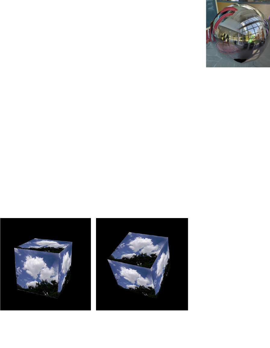
ptg11539634

Chapter 10

Advanced Techniques

This chapter includes a “grab-bag” of interesting techniques that you should find useful

for creating your WebGL applications. The techniques are mostly stand-alone, so you

can select and read any section that interests you. Where there are dependencies, they

are clearly identified. The explanations in this chapter are terse in order to include as

many techniques as possible. However, the sample programs on the website include

comprehensive comments, so please refer to them as well.

Rotate an Object with the Mouse

When creating WebGL applications, sometimes you want users to be able to control 3D

objects with the mouse. In this section, you construct a sample program

RotateObject ,

which allows users to rotate a cube by dragging it with the mouse. To make the

program simple, it uses a cube, but the basic method is applicable to any object. Figure

10.1 shows a screen shot of the cube that has a texture image mapped onto it.

Figure 10.1 A screen shot of RotateObject

ptg11539634

CHAPTER 10 Advanced Techniques

358

How to Implement Object Rotation

Rotating a 3D object is simply the application of a technique you’ve already studied for

2D objects—transforming the vertex coordinates by using the model view projection

matrix. The process requires you to create a rotation matrix based on the mouse move-

ment, change the model view projection matrix, and then transform the coordinates by

using the matrix.

You can obtain the amount of mouse movement by simply recording the position where

the mouse is initially clicked and then subtracting that position from the new position as

the mouse moves. Clearly, an event handler will be needed to calculate the mouse move-

ment, and then this will be converted into an angle that will rotate the object. Let’s take a

look at the sample program.

Sample Program (RotateObject.js)

Listing 10.1 shows the sample program. As you can see, the shaders do not do anything

special. Line 9 in the vertex shader transforms the vertex coordinates by using the model

view projection matrix, and line 10 maps the texture image onto the cube.

Listing 10.1 RotateObject.js

1 // RotateObject.js

2 // Vertex shader program

3 var VSHADER_SOURCE =

…

8 ‘void main() {n’ +

9 ‘ gl_Position = u_MvpMatrix * a_Position;n’ +

10 ‘ v_TexCoord = a_TexCoord;n’ +

11 ‘}n’;

…

24 function main() {

…

42 var n = initVertexBuffers(gl);

…

61 viewProjMatrix.setPerspective(30.0, canvas.width / canvas.height,

➥1.0, 100.0);

62 viewProjMatrix.lookAt(3.0, 3.0, 7.0, 0.0, 0.0, 0.0, 0.0, 1.0, 0.0);

64 // Register the event handler

65 var currentAngle = [0.0, 0.0]; // [x-axis, y-axis] degrees

66 initEventHandlers(canvas, currentAngle);

…

74 var tick = function() { // Start drawing

75 draw(gl, n, viewProjMatrix, u_MvpMatrix, currentAngle);

76 requestAnimationFrame(tick, canvas);

77 };

ptg11539634

Rotate an Object with the Mouse 359

78 tick();

79 }

…

138 function initEventHandlers(canvas, currentAngle) {

139 var dragging = false; // Dragging or not

140 var lastX = -1, lastY = -1; // Last position of the mouse

141

142 canvas.onmousedown = function(ev) { // Mouse is pressed

143 var x = ev.clientX, y = ev.clientY;

144 // Start dragging if a mouse is in

145 var rect = ev.target.getBoundingClientRect();

146 if (rect.left <= x && x < rect.right && rect.top <= y && y < rect.bottom) {

147 lastX = x; lastY = y;

148 dragging = true;

149 }

150 };

151 // Mouse is released

152 canvas.onmouseup = function(ev) { dragging = false; };

153

154 canvas.onmousemove = function(ev) { // Mouse is moved

155 var x = ev.clientX, y = ev.clientY;

156 if (dragging) {

157 var factor = 100/canvas.height; // The rotation ratio

158 var dx = factor * (x — lastX);

159 var dy = factor * (y — lastY);

160 // Limit x-axis rotation angle to -90 to 90 degrees

161 currentAngle[0] = Math.max(Math.min(currentAngle[0] + dy, 90.0), -90.0);

162 currentAngle[1] = currentAngle[1] + dx;

163 }

164 lastX = x, lastY = y;

165 };

166 }

167

168 var g_MvpMatrix = new Matrix4(); // The model view projection matrix

169 function draw(gl, n, viewProjMatrix, u_MvpMatrix, currentAngle) {

170 // Calculate the model view projection matrix

171 g_MvpMatrix.set(viewProjMatrix);

172 g_MvpMatrix.rotate(currentAngle[0], 1.0, 0.0, 0.0); // x-axis

173 g_MvpMatrix.rotate(currentAngle[1], 0.0, 1.0, 0.0); // y-axis

174 gl.uniformMatrix4fv(u_MvpMatrix, false, g_MvpMatrix.elements);

175

176 gl.clear(gl.COLOR_BUFFER_BIT | gl.DEPTH_BUFFER_BIT);

177 gl.drawElements(gl.TRIANGLES, n, gl.UNSIGNED_BYTE, 0);

178 }

ptg11539634

CHAPTER 10 Advanced Techniques

360

At lines 61 and 62 of main() in JavaScript, the view projection matrix is calculated in

advance. You will have to change the model matrix on-the-fly according to the amount of

mouse movement.

The code from line 65 registers the event handlers, a key part of this sample program. The

variable

currentAngle is initialized at line 65 and used to hold the current rotation angle.

Here, it is an array because it needs to handle two rotation angles around the x-axis and

y-axis. The actual registration of the event handlers is done inside

initEventHandlers() ,

called at line 66. It draws the cube using the function

tick() that is defined from line 74.

initEventHandlers() is defined at line 138. The code from line 142 handles mouse down,

the code from line 152 handles mouse up, and the code from line 154 handles the mouse

movement.

The processing when the mouse button is first pushed at line 142 is simple. Line 146

checks whether the mouse has been pressed inside the

<canvas> element. If it is inside the

<canvas> , line 147 saves that position in lastX and lastY . Then the variable dragging ,

which indicates dragging has begun, is set to

true at line 148.

The processing of the mouse button release at line 152 is simple. Because this indicates

that dragging is done, the code simply sets the variable

dragging back to false .

The processing from line 154 is the critical part and tracks the movement of the mouse.

Line 156 checks whether dragging is taking place and, if it is, lines 158 and 159 calculate

how long it has moved, storing the results to

dx and dy . These values are scaled, using

factor , which is a function of the canvas size. Once the distance dragged has been calcu-

lated, it can be used to determine the new angle by directly adding to the current angles

at line 161 and 162. The code limits rotation from –90 to +90 degrees simply to show the

technique; you are free to remove this. Because the mouse has moved, its position is saved

lastX and lastY .

Once you have successfully transformed the movement of the mouse into a rotation

angle, you can let the rotation matrix handle the updates and draw the results using

tick() . These operations are done at lines 172 and 173.

This quick review of a technique to calculate the rotation angle is only one approach.

Others, such as placing virtual track balls around the object, are described in detail in the

book 3D User Interfaces .

Select an Object

When your application requires users to be able to control 3D objects interactively, you

will need a technique to allow users to select objects. There are many uses of this tech-

nique, such as selecting a 3D button created by a 3D model instead of the conventional

2D GUI button, or selecting a photo among multiple photos in a 3D scene.

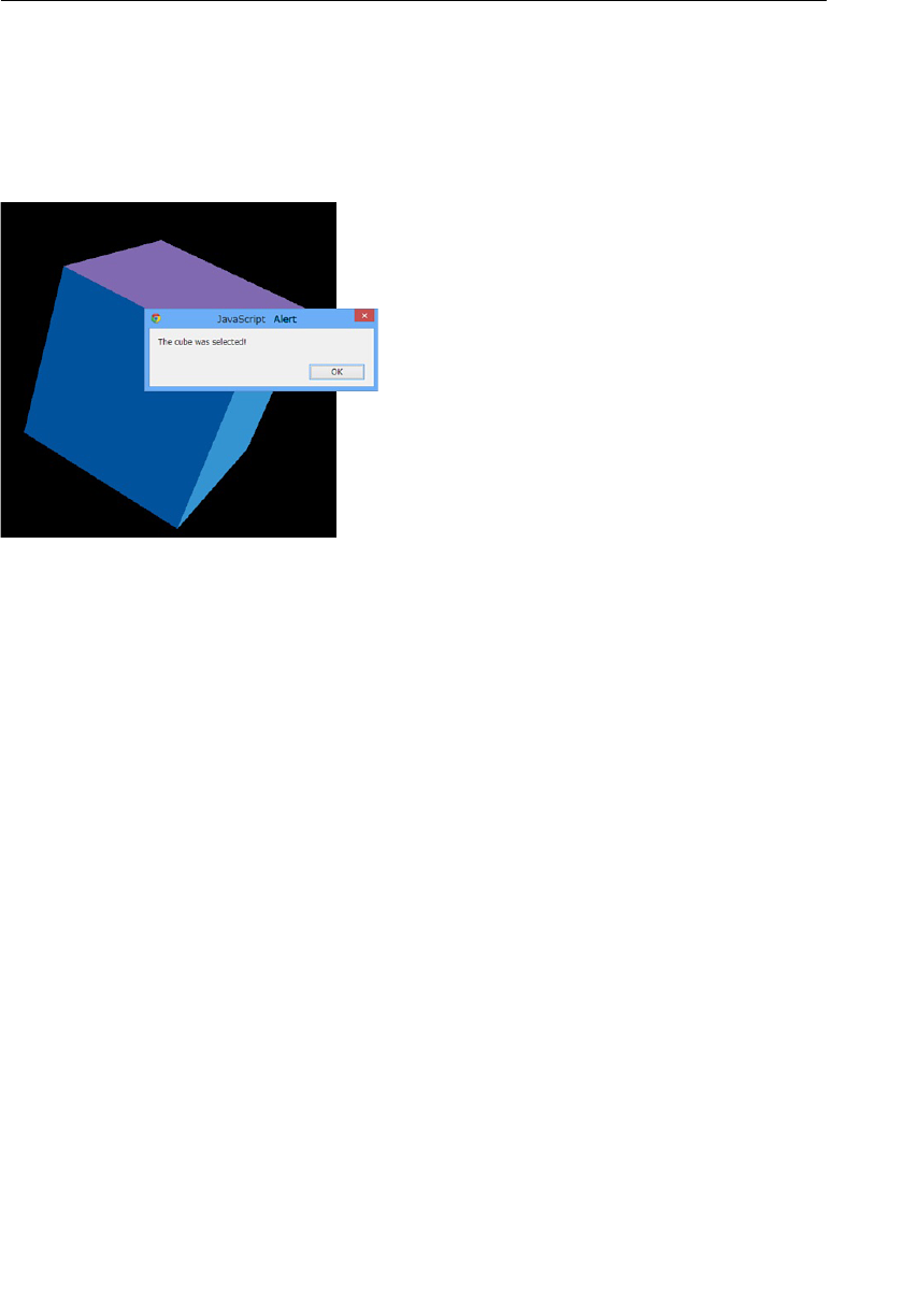
ptg11539634

Select an Object 361

Selecting a 3D object is generally more complex than selecting a 2D one because of the

mathematics required to determine if the mouse is over a nonregular shape. However,

you can use a simple trick, shown in the sample program, to avoid that complexity. In

this sample,

PickObject , the user can click a rotating cube, which causes a message to be

displayed (see Figure 10.2 ). First, run the sample program and experiment with it for a

while to get the feeling of how it works.

Figure 10.2 PickObject

Figure 10.2 shows with the message displayed when clicking the cube. The message says,

“The cube was selected!” Also check what happens when you click the black part of the

background.

How to Implement Object Selection

This program goes through the following steps to check whether the cube was clicked:

1. When the mouse is pressed, draw the cube with a single color “red” (see the middle

of Figure 10.3 ).

2. Read the pixel value (color) of the selected point.

3. Redraw the cube with its original color (right in Figure 10.3 ).

4. If the color of the pixel is red, display, “The cube was selected!”

When the cube is drawn with a single color (red in this case), you can quickly see which

part of the drawing area the cube occupies. After reading the pixel value at the position

of the mouse pointer when the mouse is clicked, you can determine that the mouse was

above the cube if the pixel color is red.

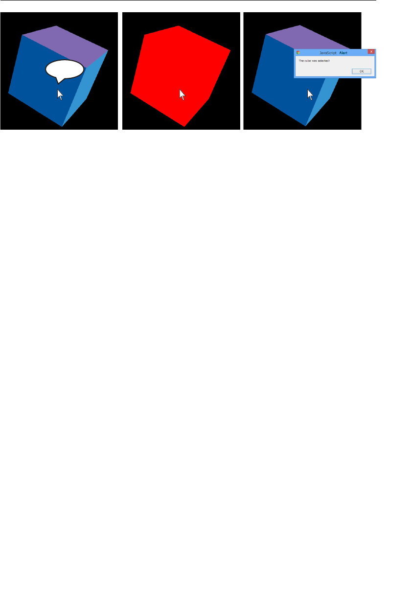
ptg11539634

CHAPTER 10 Advanced Techniques

362

Click

Figure 10.3 The object drawn at the point of mouse pressing

To ensure that the viewer doesn’t see the cube flash red, you need to draw and redraw in

the same function. Let’s take a look at the actual sample program.

Sample Program (PickObject.js)

Listing 10.2 shows the sample program. The processing in this sample mainly takes place

in the vertex shader. To implement step 1, you must inform the vertex shader that the

mouse has been clicked so that it draws the cube red. The variable

u_Clicked transmits

this information and declared at line 7 in the vertex shader. When the mouse is pressed,

u_Clicked is set to true in the JavaScript and tested at line 11. If true , the color red is

assigned to

v_Color ; if not, the color of the cube ( a_Color ) is directly assigned to v_Color .

This turns the cube red when the mouse is pressed.

Listing 10.2 PickObject.js

1 // PickObject.js

2 // Vertex shader program

3 var VSHADER_SOURCE =

…

6 ‘uniform mat4 u_MvpMatrix;n’ +

7 ‘uniform bool u_Clicked;n’ + // Mouse is pressed

8 ‘varying vec4 v_Color;n’ +

9 ‘void main() {n’ +

10 ‘ gl_Position = u_MvpMatrix * a_Position;n’ +

11 ‘ if (u_Clicked) {n’ + // Draw in red if mouse is pressed <-(1)

12 ‘ v_Color = vec4(1.0, 0.0, 0.0, 1.0);n’ +

13 ‘ } else {n’ +

14 ‘ v_Color = a_Color;n’ +

15 ‘ }n’ +

16 ‘}n’;

18 // Fragment shader program

ptg11539634

Select an Object 363

…

25 ‘ gl_FragColor = v_Color;n’ +

…

30 function main() {

…

60 var u_Clicked = gl.getUniformLocation(gl.program, ‘u_Clicked’);

…

71 gl.uniform1i(u_Clicked, 0); // Pass false to u_Clicked

73 var currentAngle = 0.0; // Current rotation angle

74 // Register the event handler

75 canvas.onmousedown = function(ev) { // Mouse is pressed

76 var x = ev.clientX, y = ev.clientY;

77 var rect = ev.target.getBoundingClientRect();

78 if (rect.left <= x && x < rect.right && rect.top <= y && y < rect.bottom) {

79 // Check if it is on object

80 var x_in_canvas = x — rect.left, y_in_canvas = rect.bottom — y;

81 var picked = check(gl, n, x_in_canvas, y_in_canvas, currentAngle,

➥u_Clicked, viewProjMatrix, u_MvpMatrix);

82 if (picked) alert(‘The cube was selected! ‘); <-(4)

83 }

84 }

…

92 }

…

147 function check(gl, n, x, y, currentAngle, u_Clicked, viewProjMatrix,

➥u_MvpMatrix) {

148 var picked = false;

149 gl.uniform1i(u_Clicked, 1); // Draw the cube with red

150 draw(gl, n, currentAngle, viewProjMatrix, u_MvpMatrix);

151 // Read pixel at the clicked position

152 var pixels = new Uint8Array(4); // Array for storing the pixels

153 gl.readPixels(x, y, 1, 1, gl.RGBA, gl.UNSIGNED_BYTE, pixels); <-(2)

154

155 if (pixels[0] == 255) // The mouse in on cube if pixels[0] is 255

156 picked = true;

157

158 gl.uniform1i(u_Clicked, 0); // Pass false to u_Clicked: redraw cube

159 draw(gl, n, currentAngle, viewProjMatrix, u_MvpMatrix); // <-(3)

160

161 return picked;

162 }

Let’s take a look from line 30 of main() in JavaScript. Line 60 obtains the storage location

for

u_Clicked , and line 71 assigns the initial value of u_Clicked to be false .

ptg11539634

CHAPTER 10 Advanced Techniques

364

Line 75 registers the event handler to be called when the mouse has been clicked. This

event handler function does a sanity check to see if the clicked position is inside the

<canvas> element at line 78. Then it calls to check() at line 81 if it is. This function checks

whether the position, specified by the third and fourth arguments, is on the cube (see next

paragraph). If so, it returns

true which causes a message to be displayed at line 82.

The function check() begins from line 147. This function processes steps (2) and (3) from

the previous section together. Line 149 informs the vertex shader that the click event has

occurred by passing 1 (

true ) to u_Clicked . Then line 150 draws the cube with the current

rotation angle. Because

u_Clicked is true , the cube is drawn in red. Then the pixel value

of the clicked position is read from the color buffer at line 153. The following shows the

gl.readPixels() function used here.

gl.readPixels(x, y, width, height, format, type, pixels)

Read a block of pixels from the color buffer

1 and store it to the array pixels . x , y , width ,

and height define the block as a rectangle.

Parameters x, y Specify the position of the first pixel that is read from the

buffer.

width, height Specify the dimensions of the pixel rectangle.

format Specifies the format of the pixel data.

gl.RGBA must be

specified.

type Specifies the data type of the pixel data.

gl.UNSIGNED_BYTE

must be specified.

pixels Specifies the typed array (

Uint8Array ) for storing the pixel

data.

Return value None

Errors INVALID_VALUE: pixels is

null . Either width or height is negative.

INVALID_OPERATION: pixels is not large enough to store the pixel data.

INVALID_ENUM: format or type is none of the above values.

The pixel value that was read is stored in the pixels array. This array is defined at line

152, and the R, G, B, and A values are stored in

pixels[0] , pixels[1] , pixels[2] , and

pixels[3] , respectively. Because, in this sample program, you know that the only colors

used are red for the cube and black for the background, you can see if the mouse is on

the cube by checking the values for

pixels[0] . This is done at line 155, and if it is red, it

changes

picked to true .

1 If a framebuffer object is bound to gl.FRAMEBUFFER , this method reads the pixel values from the

object. We explain the object in the later section “Use What You’ve Drawn as a Texture Image.”

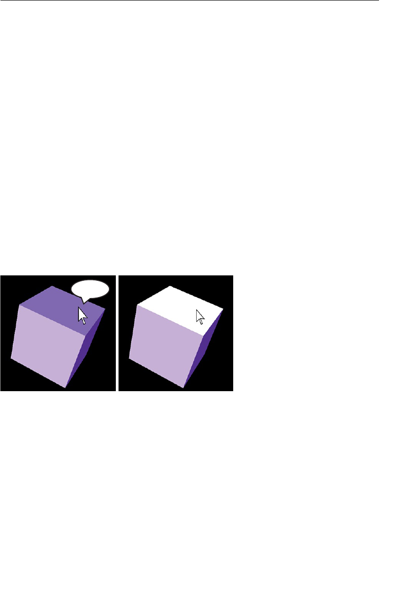
ptg11539634

Select an Object 365

Then line 158 sets u_Clicked to false and redraws the cube at line 159. This turns the

cube back to its original color. Line 161 returns

picked as the return value.

Note, if at this point you call any function that returns control to the browser, such as

alert() , the content of the color buffer will be displayed on the <canvas> at that point.

For example, if you execute

alert(‘The cube was selected!’) at line 156, the red cube

will be displayed when you click the cube.

This approach, although simple, can handle more than one object by assigning differ-

ent colors to each object. For example, red, blue, and green are enough if there are three

objects. For larger numbers of objects, you can use individual bits. Because there are 8 bits

for each component in RGBA, you can represent 255 objects just by using the R compo-

nent. However, if the 3D objects are complex or the drawing area is large, it will take

some time to process the selection of objects. To overcome this disadvantage, you can use

simplified models to select objects or shrink the drawing area. In such cases, you can use

the framebuffer object, which will be explained in the section “Use What You’ve Drawn as

a Texture Image” later in this chapter.

Select the Face of the Object

You can also apply the method explained in the previous section to select a particular

face of an object. Let’s customize

PickObject to build PickFace , a program that turns the

selected face white. Figure 10.4 shows

PickFace .

Click

Figure 10.4 PickFace

PickFace is easy once you understand how PickObject works. PickObject drew the cube

in red when the mouse was clicked, resulting in the object’s display area in the color

buffer being red. By reading the pixel value of the clicked point and seeing if the color

of the pixel at the position was red, the program could determine if the object had been

selected.

PickFace goes one step further and inserts the information of which face has

been selected into the color buffer. Here, you will insert the information in the alpha

component of the RGBA value. Let’s take a look at the sample program.

ptg11539634

CHAPTER 10 Advanced Techniques

366

Sample Program (PickFace.js)

PickFace.js is shown in Listing 10.3 . Some parts, such as the fragment shader, are

omitted for brevity.

Listing 10.3 PickFace.js

1 // PickFace.js

2 // Vertex shader program

3 var VSHADER_SOURCE =

4 ‘attribute vec4 a_Position;n’ +

5 ‘attribute vec4 a_Color;n’ +

6 ‘attribute float a_Face;n’ + // Surface number (Cannot use int)

7 ‘uniform mat4 u_MvpMatrix;n’ +

8 ‘uniform int u_PickedFace;n’ + // Surface number of selected face

9 ‘varying vec4 v_Color;n’ +

10 ‘void main() {n’ +

11 ‘ gl_Position = u_MvpMatrix * a_Position;n’ +

12 ‘ int face = int(a_Face);n’ + // Convert to int

13 ‘ vec3 color = (face == u_PickedFace) ? vec3(1.0):a_Color.rgb;n’+

14 ‘ if(u_PickedFace == 0) {n’ + // Insert face number into alpha

15 ‘ v_Color = vec4(color, a_Face/255.0);n’ +

16 ‘ } else {n’ +

17 ‘ v_Color = vec4(color, a_Color.a);n’ +

18 ‘ }n’ +

19 ‘}n’;

…

33 function main() {

…

50 // Set vertex information

51 var n = initVertexBuffers(gl);

…

74 // Initialize selected surface

75 gl.uniform1i(u_PickedFace, -1);

77 var currentAngle = 0.0; // Current rotation angle (degrees)

78 // Register event handlers

79 canvas.onmousedown = function(ev) { // Mouse is pressed

80 var x = ev.clientX, y = ev.clientY;

81 var rect = ev.target.getBoundingClientRect();

82 if (rect.left <= x && x < rect.right && rect.top <= y && y < rect.bottom) {

83 // If clicked position is inside the

, update the face

84 var x_in_canvas = x — rect.left, y_in_canvas = rect.bottom — y;

85 var face = checkFace(gl, n, x_in_canvas, y_in_canvas,

➥currentAngle, u_PickedFace, viewProjMatrix, u_MvpMatrix);

86 gl.uniform1i(u_PickedFace, face); // Pass the surface number

87 draw(gl, n, currentAngle, viewProjMatrix, u_MvpMatrix);

ptg11539634

Select an Object 367

88 }

89 }

…

99 function initVertexBuffers(gl) {

…

109 var vertices = new Float32Array([ // Vertex coordinates

110 1.0, 1.0, 1.0, -1.0, 1.0, 1.0, -1.0,-1.0, 1.0, 1.0,-1.0, 1.0,

111 1.0, 1.0, 1.0, 1.0,-1.0, 1.0, 1.0,-1.0,-1.0, 1.0, 1.0,-1.0,

…

115 1.0,-1.0,-1.0, -1.0,-1.0,-1.0, -1.0, 1.0,-1.0, 1.0, 1.0,-1.0

116 ]);

…

127 var faces = new Uint8Array([ // Surface number

128 1, 1, 1, 1, // v0-v1-v2-v3 Front

129 2, 2, 2, 2, // v0-v3-v4-v5 Right

…

133 6, 6, 6, 6, // v4-v7-v6-v5 Depth

134 ]);

…

154 if (!initArrayBuffer(gl, faces, gl.UNSIGNED_BYTE, 1,

➥‘a_Face’)) return -1; // Surface Information

…

164 }

165

166 function checkFace(gl, n, x, y, currentAngle, u_PickedFace, viewProjMatrix,

➥u_MvpMatrix) {

167 var pixels = new Uint8Array(4); // Array for storing the pixel

168 gl.uniform1i(u_PickedFace, 0); // Write surface number into alpha

169 draw(gl, n, currentAngle, viewProjMatrix, u_MvpMatrix);

170 // Read the pixels at (x, y). pixels[3] is the surface number

171 gl.readPixels(x, y, 1, 1, gl.RGBA, gl.UNSIGNED_BYTE, pixels);

172

173 return pixels[3];

174 }

Let’s take a look from the vertex shader. a_Face at line 6 is the attribute variable used to

pass the surface number, which is then “coded” into the alpha value when the mouse

is clicked. The surface numbers are set up in

initVertexBuffers() defined at line 99

and simply map vertices to a surface. Lines 127 onward define these mappings. So, for

example, vertices v0-v1-v2-v3 define a surface that is numbered 1, vertices v0-v3-v4-v5 are

numbered 2, and so on. Because each vertex needs a number to pass to the vertex shader,

there are four 1s written at line 128 to represent the first face.

If a face is already selected,

u_PickedFace at line 8 informs the vertex shader of the

selected face number, allowing the shader to switch the way it draws the face based on

this information.

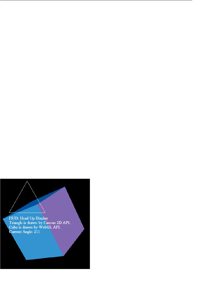
ptg11539634

CHAPTER 10 Advanced Techniques

368

Line 12 converts a_Face , the surface number that is a float type, into an int type because

int type cannot be used in the attribute variables ( Chapter 6 , “The OpenGL ES Shading

Language [GLSL ES]”). If the selected surface number is the same as the surface number

currently being manipulated, white is assigned to

color at line 13. Otherwise, the original

surface color is assigned. If the mouse has been clicked (that is,

u_PickedFace is set to 0),

the

a_Face value is inserted into the alpha value and the cube is drawn (line 15).

Now, by passing 0 into u_PickedFace when the mouse is clicked, the cube is drawn with

an alpha value set to the surface number.

u_PickedFace is initialized to –1 at line 75.

There is no surface with the number –1 (refer to the

faces array at line 127), so the cube is

initially drawn without surfaces selected.

Let’s take a look at the essential processing of the event handler.

u_PickedFace is passed

as an argument to

checkFace() at line 85, which returns the surface number of the picked

face,

checkFace() , at line 166. At line 168, 0 is passed to u_PickedFace to tell the vertex

shader that the mouse has been clicked. When

draw() is called in the next line, the

surface number is inserted into the alpha value and the object is redrawn. Line 171 checks

the pixel value of the clicked point, and line 173 retrieves the inserted surface number

by using

pixels[3] . (It is the alpha value, so the subscript is 3.) This surface number is

returned to the main code and then used at lines 86 and 87 to draw the cube. The vertex

shader handles the rest of the processing, as described earlier.

HUD (Head Up Display)

The Head Up Display, originally developed for aircraft, is a transparent display that pres-

ents data without requiring users to look away from their usual viewpoints. A similar

effect can be achieved in 3D graphics and used to overlay textual information on the 3D

scene. Here, you will construct a sample program that will display a diagram and some

information on top of the 3D graphics (HUD), as you can see in Figure 10.5 .

Figure 10.5 HUD

ptg11539634

HUD (Head Up Display) 369

The goal of the program is to draw a triangle and some simple information about the 3D

scene, including the current rotation angle of the cube (from

PickObject ) that will change

as the cube rotates.

How to Implement a HUD

This HUD effect can be implemented using HTML and the canvas function without

WebGL. This is done as follows:

1. In the HTML file, prepare a

<canvas> to draw the 3D graphics using WebGL and

another

<canvas> to draw the HUD using the canvas function. In other words,

prepare two

<canvas> and place the HUD on top of the WebGL canvas.

2. Draw the 3D graphics using the WebGL API on the <canvas> for WebGL.

3. Draw the HUD using the canvas functions on the

<canvas> for the HUD.

As you can see, this is extremely simple and shows the power of WebGL and its ability to

mix 2D and 3D graphics within the browser. Let’s take a look at the sample program.

Sample Program (HUD.html)

Because we need to make changes to the HTML file to add the extra canvas, we show HUD.

html in Listing 10.4 , with the additions in bold.

Listing 10.4 HUD.html

1 <!DOCTYPE html>

2 <html lang=»ja»>

…

8 <body onload=»main()»>

9 <canvas id=»webgl» width=»400″ height=»400″ style=»position:

➥absolute; z-index: 0″ >

10 Please use a browser that supports

«canvas»

11 </canvas>

12 <canvas id=»hud» width=»400″ height=»400″ style=»position:

➥absolute;z-index: 1″></canvas>

…

18 <script src=»HUD.js»></script>

19 </body>

20 </html>

The style attribute, used to define how an element looks or how it is arranged, allows you

to place the HUD canvas on top of the WebGL canvas. Style information is composed of

the property name and the value separated with a

: as seen at line 9: style=»position:

absolute» . Multiple style elements are separated with ; .

ptg11539634

CHAPTER 10 Advanced Techniques

370

In this example, you use position , which specifies how the element is placed, and the

z-index , which specifies the hierarchical relationship.

You can specify the position of the element in the absolute coordinate if you use absolute

for the

position value. Unless you specify the position, all the elements specified to this

attribute will be place at the same position.

z-index specifies the order in which elements

are displayed when multiple elements are at the same position. The element with the

larger number will be displayed over the one with a smaller number. In this case, the

z-index of the <canvas> for the HUD at line 12 is 1.

The result of this code is two <canvas> elements, placed at the same location with

the

<canvas> that displays the HUD on top of the <canvas> that displays the WebGL.

Conveniently, the background of the canvas element is transparent by default, so the

WebGL canvas can be seen through the HUD canvas. Anything that is drawn on the HUD

canvas will appear over the 3D objects and create the effect of a HUD.

Sample Program (HUD.js)

Next, let’s take a look at HUD.js in Listing 10.5 . There are two changes made compared to

PickObject.js :

1. Retrieve the rendering context to draw in the <canvas> for the HUD and use it to

draw.

2. Register the event handler when the mouse is clicked to the

<canvas> for the HUD

and not to the

<canvas> for WebGL.

Step 1 simply uses the source code used in Chapter 2 , “Your First Step with WebGL,” to

draw a triangle onto the

<canvas> . Step 2 is required to ensure that mouse click informa-

tion is passed to the HUD canvas rather than the WebGL canvas. The vertex shader and

fragment shader are the same as

PickObject.js .

Listing 10.5 HUD.js

1 // HUD.js

…

30 function main() {

31 // Retrieve

element

32 var canvas = document.getElementById(‘webgl’);

33 var hud = document.getElementById(‘hud’);

…

40 // Get the rendering context for WebGL

41 var gl = getWebGLContext(canvas);

42 // Get the rendering context for 2DCG

43 var ctx = hud.getContext(‘2d’);

…

82 // Register the event handler

83 hud.onmousedown = function(ev) { // Mouse is pressed

ptg11539634

HUD (Head Up Display) 371

…

89 check(gl, n, x_in_canvas, y_in_canvas, currentAngle, u_Clicked,

➥viewProjMatrix, u_MvpMatrix);

…

91 }

93 var tick = function() { // Start drawing

94 currentAngle = animate(currentAngle);

95 draw2D(ctx, currentAngle); // Draw 2D

96 draw(gl, n, currentAngle, viewProjMatrix, u_MvpMatrix);

97 requestAnimationFrame(tick, canvas);

98 };

99 tick();

100 }

…

184 function draw2D(ctx, currentAngle) {

185 ctx.clearRect(0, 0, 400, 400); // Clear <hud>

186 // Draw triangle with white lines

187 ctx.beginPath(); // Start drawing

188 ctx.moveTo(120, 10); ctx.lineTo(200, 150); ctx.lineTo(40, 150);

189 ctx.closePath();

190 ctx.strokeStyle = ‘rgba(255, 255, 255, 1)’; // Set the line color

191 ctx.stroke(); // Draw triangle with white lines

192 // Draw white letters

193 ctx.font = ’18px «Times New Roman»‘;

194 ctx.fillStyle = ‘rgba(255, 255, 255, 1)’; // Set the letter color

195 ctx.fillText(‘HUD: Head Up Display’, 40, 180);

196 ctx.fillText(‘Triangle is drawn by Hud API.’, 40, 200);

197 ctx.fillText(‘Cube is drawn by WebGL API.’, 40, 220);

198 ctx.fillText(‘Current Angle: ‘+ Math.floor(currentAngle), 40, 240);

199 }

Because the processing flow of the program is straightforward, let’s take a look from

main() at line 30. First, line 33 obtains the <canvas> element for the HUD. This is used to

get the drawing context for the 2D graphics ( Chapter 2 ) at line 43, which is used to draw

the HUD. You register the mouse-click event handler for the HUD canvas (

hud ) instead of

the WebGL canvas in

PickObject.js . This is because the event goes to the HUD canvas,

which is placed on top of the WebGL canvas.

The code from line 93 handles the animation and uses

draw2D() , added at line 95, to draw

the HUD information.

draw2D() is defined at line 184 and takes ctx parameters, the context to draw on the

canvas, and the current rotation angle,

currentAngle . Line 185 clears the HUD canvas

using the

clearRect() method, which takes the upper-left corner, the width, and the

height of the rectangle to clear. Lines 187 to 191 draw the triangle which, unlike drawing

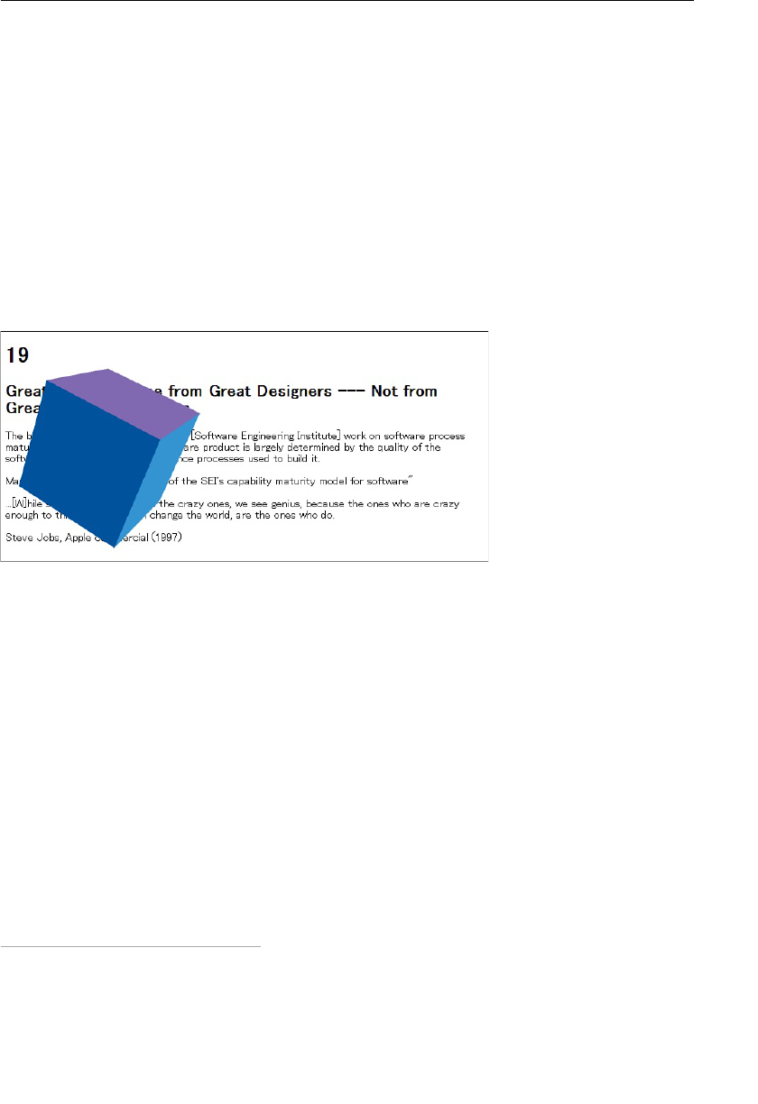
ptg11539634

CHAPTER 10 Advanced Techniques

372

a rectangle as explained in Chapter 2 , requires that you define the path (outline) of a

triangle to draw it. Lines 187 to 191 define the path, set the color, and draw the triangle.

Lines 193 onward specify the text color and font and then use

fillText() , which speci-

fies the letters to draw as the first parameter and the x and y coordinates to draw as the

second and third parameters, to actually write the text. Line 198 displays the current

rotation angle and uses

Math.floor() to truncate the numbers below the decimal point.

Line 185 clears the canvas because the displayed value (rotation angle) changes at each

drawing.

Display a 3D Object on a Web Page (3DoverWeb)

Displaying a 3D object on a web page is simple with WebGL and the inverse of the HUD

example. In this case, the WebGL canvas is on top of the web page, and the canvas is set

to transparent. Figure 10.6 shows

3DoverWeb .

Figure 10.6 3DoverWeb

3DoverWeb.js is based on PickObject.js with almost no changes. The only change is that

the alpha value of the clear color is changed from 1.0 to 0.0 at line 55.

55 gl.clearColor(0.0, 0.0, 0.0, 0.0 );

By making the alpha value 0.0, the background of the WebGL canvas becomes transpar-

ent, and you can see the web page behind the WebGL

<canvas> . You can also experiment

with the alpha value; any value other than 1.0 changes the transparency and makes the

web page more or less visible.

Fog (Atmospheric Effect)

In 3D graphics, the term fog is used to describe the effect that makes a distant object seem

hazy. The term describes objects in any medium, so objects underwater can also have a

2 The sentences on the web page on the background are from the book The Design of Design (by

Frederick P. Brooks Jr, Pearson).

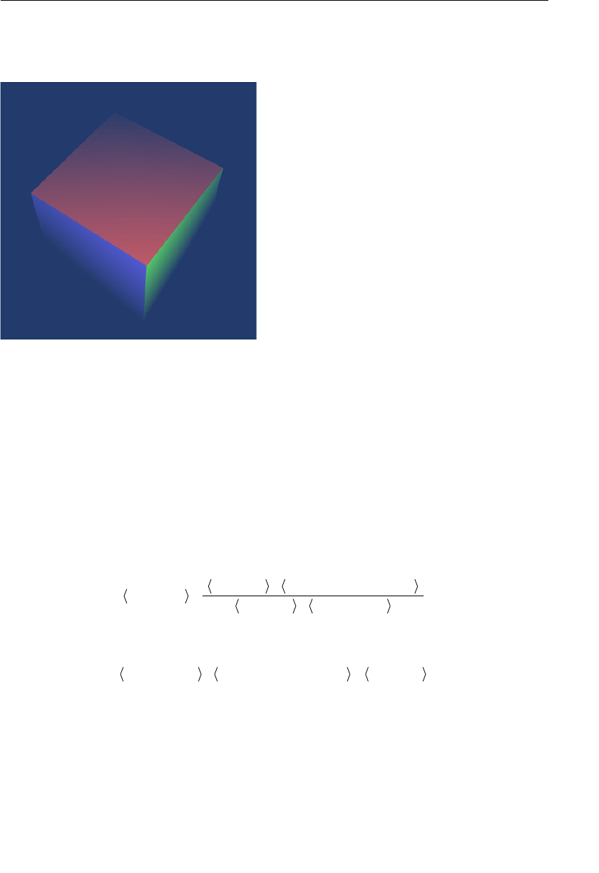
ptg11539634

Fog (Atmospheric Effect) 373

fog effect applied. Here, you construct a sample program Fog that realizes the fog effect.

Figure 10.7 shows a screen shot. You can adjust the density of the fog with the up/down

arrow keys. Try running the sample program and experiment with the effect.

Figure 10.7 Fog

How to Implement Fog

There are various ways to calculate fog, but here you will use a linear computation ( linear

fog ) because the calculation is easy. The linear fog method determines the density of the

fog by setting the starting point (the distance where the object starts to become hazy) and

the end point (where the object is completely obscured). The density of the fog between

these points is changed linearly. Note that the end point is not where the fog ends; rather,

it is where the fog becomes so dense that it obscures all objects. We will call how clearly

we can see the object the fog factor ; it is calculated, in the case of linear fog, as follows:

Equation 10.1

()

=−

−

fog factor end point distance from eye point

end point starting point







Where

≤≤starting point distance from eye point end point

When the fog factor is 1.0, you can see the object completely, and if it 0.0, you cannot see

it at all (see Figure 10.8 ). The fog factor is 1.0 when the (distance from eye point)

(starting point) , and 0.0 when (end point) < (distance from eye point) .

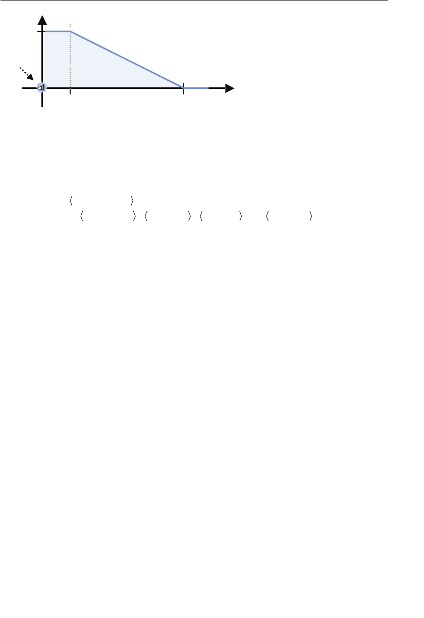
ptg11539634

CHAPTER 10 Advanced Techniques

374

rotcaf gof

morf ecnatsid

tniop eye

ecnatsid dne

ecnatsid trats

0.1

eye point

Figure 10.8 Fog factor

You can calculate the color of a fragment based on the fog factor, as follows in Equation

10.2 .

Equation 10.2

()

×+×−

fragment color

surface color fog factor fog color fog factor



 1

Now, let’s take a look at the sample program.

Sample Program (Fog.js)

The sample program is shown in Listing 10.6 . Here, you (1) calculate the distance of the

object (vertex) from the eye point in the vertex shader, and based on that, you (2) calcu-

late the fog factor and the color of the object based on the fog factor in the fragment

shader. Note that this program specifies the position of the eye point with the world

coordinate system (see Appendix G , “World Coordinate System Versus Local Coordinate

System”) so the fog calculation takes place in the world coordinate system.

Listing 10.6 Fog.js

1 // Fog.js

2 // Vertex shader program

3 var VSHADER_SOURCE =

…

7 ‘uniform mat4 u_ModelMatrix;n’ +

8 ‘uniform vec4 u_Eye;n’ + // The eye point (world coordinates)

9 ‘varying vec4 v_Color;n’ +

10 ‘varying float v_Dist;n’ +

11 ‘void main() {n’ +

12 ‘ gl_Position = u_MvpMatrix * a_Position;n’ +

13 ‘ v_Color = a_Color;n’ +

14 // Calculate the distance to each vertex from eye point <-(1)

15 ‘ v_Dist = distance(u_ModelMatrix * a_Position, u_Eye);n’ +

16 ‘}n’;

ptg11539634

Fog (Atmospheric Effect) 375

18 // Fragment shader program

19 var FSHADER_SOURCE =

…

23 ‘uniform vec3 u_FogColor;n’ + // Color of Fog

24 ‘uniform vec2 u_FogDist;n’ + // Fog starting point, end point)

25 ‘varying vec4 v_Color;n’ +

26 ‘varying float v_Dist;n’ +

27 ‘void main() {n’ +

28 // Calculate the fog factor <-(2)

29 ‘ float fogFactor = clamp((u_FogDist.y — v_Dist) / (u_FogDist.y –

➥u_FogDist.x), 0.0, 1.0);n’ +

30 // u_FogColor * (1 — fogFactor) + v_Color * fogFactor

31 ‘ vec3 color = mix(u_FogColor, vec3(v_Color), fogFactor);n’ +

32 ‘ gl_FragColor = vec4(color, v_Color.a);n’ +

33 ‘}n’;

35 function main() {

…

53 var n = initVertexBuffers(gl);

…

59 // Color of fog

60 var fogColor = new Float32Array([0.137, 0.231, 0.423]);

61 // Distance of fog [fog starts, fog completely covers object]

62 var fogDist = new Float32Array([55, 80]);

63 // Position of eye point (world coordinates)

64 var eye = new Float32Array([25, 65, 35]);

…

76 // Pass fog color, distances, and eye point to uniform variable

77 gl.uniform3fv(u_FogColor, fogColor); // Fog color

78 gl.uniform2fv(u_FogDist, fogDist); // Starting point and end point

79 gl.uniform4fv(u_Eye, eye); // Eye point

81 // Set clear color and enable hidden surface removal function

82 gl.clearColor( fogColor[0], fogColor[1], fogColor[2] , 1.0);

…

93 mvpMatrix.lookAt( eye[0], eye[1], eye[2] , 0, 2, 0, 0, 1, 0);

…

97 document.onkeydown = function(ev){ keydown(ev, gl, n, u_FogDist, fogDist); };

…

The calculation of the distance from the eye point to the vertex, done by the vertex

shader, is straightforward. You simply transform the vertex coordinates to the world coor-

dinates using the model matrix and then call the built-in function

distance() with the

position of the eye point (world coordinates) and the vertex coordinates. The

distance()

ptg11539634

CHAPTER 10 Advanced Techniques

376

function calculates the distance between two coordinates specified by the arguments. This

calculation takes place at line 15, and the result is then written to the

v_Dist variable and

passed to the fragment shader.

The fragment shader calculates the fogged color of the object using Equations 10.1 and

10.2 . The fog color, fog starting point, and fog end point, which are needed to calculate

the fogged color, are passed in the uniform variables

u_FogColor and u_FogDist at lines 23

and 24.

u_FogDist.x is the starting point, and u_FogDist.y is the end point.

The fog factor is calculated at line 29 using Equation 10.1 . The clamp() function is a built-

in function; if the value specified by the first parameter is outside the range specified by

the second and third parameter ([0.0 0.1] in this case), it will fix the value to one within

the range. In other words, the value is fixed to 0.0 if the value is smaller than 0.0, and 1.0

if the value is larger than 1.0. If the value is within the range, the value is unchanged.

Line 31 is the calculation of the fragment color using the fog factor. This implements

Equation 10.2 and uses a built-in function,

mix() , which calculates x*(1–z)+y*z, where x is

the first parameter, y is the second, and z is the third.

The processing in JavaScript’s

main() function from line 35 sets up the values necessary

for calculating the fog in the appropriate uniform variables.

You should note that there are many types of fog calculations other than linear fog, for

example exponential fog, used in OpenGL (see the book OpenGL Programming Guide ). You

can implement these fog calculations using the same approach, just changing the calcula-

tion method in the fragment shader.

Use the w Value (Fog_w.js)

Because the distance calculation within the shader can affect performance, an alternative

method allows you to easily approximate the calculation of the distance from the eye

point to the object (vertex) by using the w value of coordinates transformed by the model

view projection conversion. In this case, the coordinates are substituted in

gl_Position .

The fourth component, w of

gl_Position which you haven’t used explicitly before, is the

z value of each vertex in the view coordinate system multiplied by –1. The eye point is the

origin in the view coordinates, and the view direction is the negative direction of z, so z

is a negative value. The w value, which is the z value multiplied by –1, can be used as an

approximation of the distance.

If you reimplement the calculation in the vertex shader using w, as shown in Listing 10.7 ,

the fog effect will work as before.

Listing 10.7 Fog_w.js

1 // Fog_w.js

2 // Vertex shader program

3 var VSHADER_SOURCE =

…

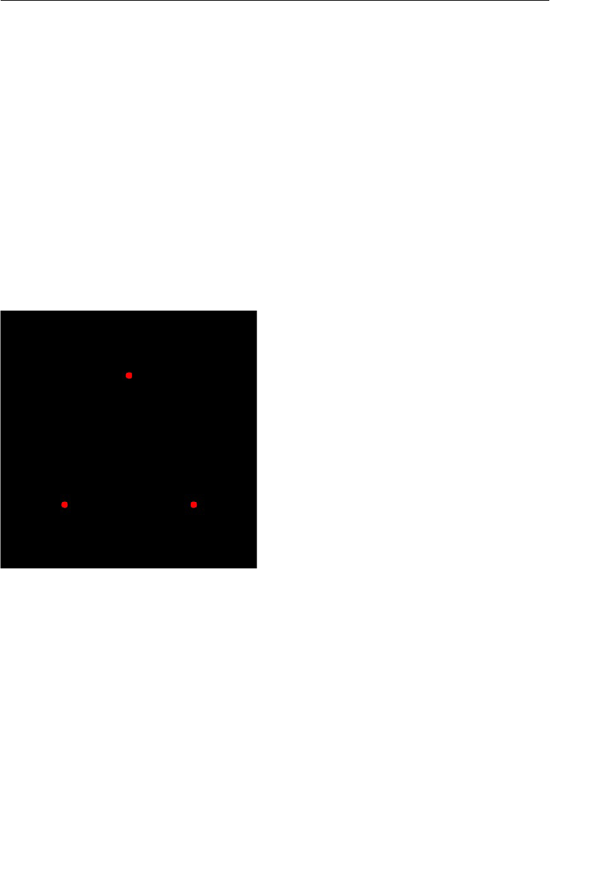
ptg11539634

Make a Rounded Point 377

7 ‘varying vec4 v_Color;n’ +

8 ‘varying float v_Dist;n’ +

9 ‘void main() {n’ +

10 ‘ gl_Position = u_MvpMatrix * a_Position;n’ +

11 ‘ v_Color = a_Color;n’ +

12 // Use the negative z value of vertex in view coordinate system

13 ‘ v_Dist = gl_Position.w;n’ +

14 ‘}n’;

Make a Rounded Point

In Chapter 2 , you constructed a sample program that draws a point to help you under-

stand the basics of shaders. However, to allow you to focus on the operation of the

shaders, the point displayed wasn’t “round” but actually “square,” which is simpler to

draw. In this section, you construct a sample program,

RoundedPoint , which draws a

round point (see Figure 10.9 ).

Figure 10.9 A screen shot of RoundedPoint

How to Implement a Rounded Point

To draw a “round” point, you just have to make the “rectangle” point round. This can be

achieved using the rasterization process that takes place between the vertex shader and

the fragment shader and was explained in Chapter 5 , “Using Colors and Texture Images.”

This rasterization process generates a rectangle consisting of multiple fragments, and each

fragment is passed to the fragment shader. If you draw these fragments as-is, a rectangle

will be displayed. So you just need to modify the fragment shader to draw only the frag-

ments inside the circle, as shown in Figure 10.10 .

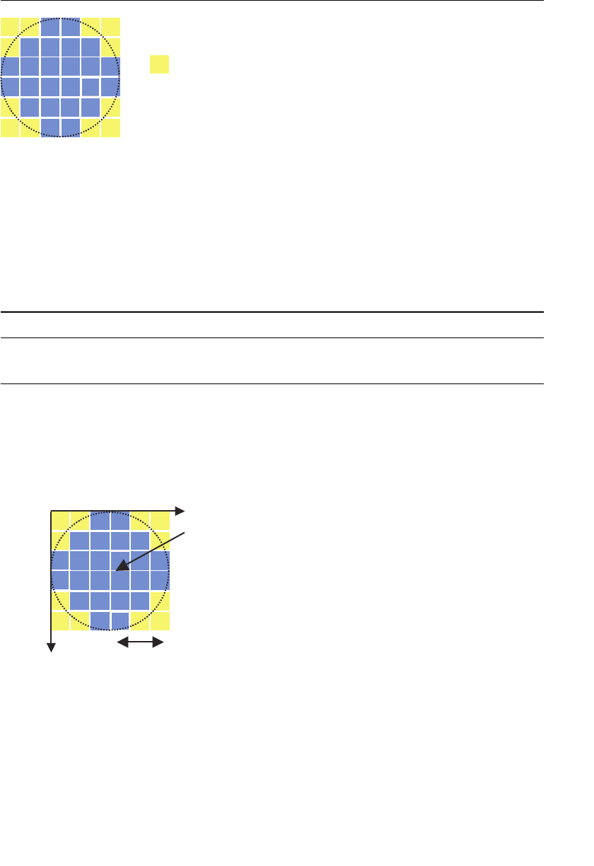
ptg11539634

CHAPTER 10 Advanced Techniques

378

dedracsidebotstnemgarf

Figure 10.10 Discarding fragments to turn a rectangle into a circle

To achieve this, you need to know the position of each fragment created during rasteriza-

tion. In Chapter 5 , you saw a sample program that uses the built-in variable

gl_FragCoord

to pass (input) the data to the fragment shader. In addition to this, there is one more

built-in variable

gl_PointCoord , which is suitable for drawing a round point (see Table

10.1 ).

Table 10.1 Built-In Variables of Fragment Shader (Input)

Type and Name of Variable Description

vec4 gl_FragCoord Window coordinates of fragment

vec4 gl_PointCoord Position of fragment in the drawn point (0.0 to 1.0)

gl_PointCoord gives the position of each fragment taken from the range (0.0, 0.0) to (1.0,

1.0), as shown in Figure 10.11 . To make the rectangle round, you simply have to discard

the fragments outside the circle centered at (0.5, 0.5) with radius 0.5. You can use the

discard statement to discard these fragments.

)5.0,5.0(

5.0

)0.0,0.0(

)0.1,0.1(

Figure 10.11 Coordinates of gl_PointCoord

Sample Program (RoundedPoints.js)

The sample program is shown in Listing 10.8 . This is derived from MultiPoint.js , which

was used in Chapter 4 , “More Transformations and Basic Animation,” to draw multiple

ptg11539634

Make a Rounded Point 379

points. The only difference is in the fragment shader. The vertex shader is also shown for

reference.

Listing 10.8 RoundedPoint.js

1 // RoundedPoints.js

2 // Vertex shader program

3 var VSHADER_SOURCE =

4 ‘attribute vec4 a_Position;n’ +

5 ‘void main() {n’ +

6 ‘ gl_Position = a_Position;n’ +

7 ‘ gl_PointSize = 10.0;n’ +

8 ‘}n’;

10 // Fragment shader program

11 var FSHADER_SOURCE =

…

15 ‘void main() {n’ + // Center coordinate is (0.5, 0.5)

16 ‘ float dist = distance(gl_PointCoord, vec2(0.5, 0.5));n’ +

17 ‘ if(dist < 0.5) {n’ + // Radius is 0.5

18 ‘ gl_FragColor = vec4(1.0, 0.0, 0.0, 1.0);n’ +

19 ‘ } else { discard; }n’ +

20 ‘}n’;

22 function main() {

…

53 gl.drawArrays(gl.POINTS, 0, n);

54 }

The key difference is the calculation, starting at line 16, which determines whether a frag-

ment should be discarded.

gl_PointCoord holds the fragment’s position (specified in the

range 0.0 to 0.1), and the center point is (0.5, 0.5). Therefore, to make a rectangle point

round, you have to do the following:

1. Calculate the distance from the center (0.5, 0.5) to each fragment.

2. Draw those fragments for which the distance is less than 0.5.

RoundedPoint.js , the distance calculation takes place at line 16. Here, you just have to

calculate the distance between the center point (0.5, 0.5) and

gl_PointCoord . Because the

gl_PointCoord is a vec2 type, you need to pass (0.5, 0.5) to distance() as a vec2 .

Once you have calculated the distance from the center, it is used at line 17 to check

whether the distance is less than 0.5 (in other words, whether the fragment is in the

circle). If the fragment is in circle, the fragment is drawn so line 18 uses

gl_FragColor to

set the draw color. Otherwise, at line 19, the

discard statement causes WebGL to auto-

matically throw away the fragment.

ptg11539634

CHAPTER 10 Advanced Techniques

380

Alpha Blending

The alpha value controls the transparency of drawn objects. If you specify 0.5 as the alpha

value, the object becomes semi-transparent, allowing anything drawn underneath it to be

partially visible. As the alpha value approaches 0, more of the background objects appear.

If you try this yourself, you’ll actually see that as you decrease the alpha value, WebGL

objects become white. This is because WebGL’s default behavior is to use the same alpha

value for both objects and the

<canvas> . In the sample programs, the web page behind

the

<canvas> is white, so this shows through.

Let’s construct a sample program that shows how to use alpha blending to get the desired

effect. The function that allows the use of the alpha value is called an alpha blending (or

simply blending ) function . This function is already built into WebGL, so you just need to

enable it to tell WebGL to start to use the alpha values supplied.

How to Implement Alpha Blending

You’ll need the following two steps to enable and use the alpha blending function.

1. Enable the alpha blending function:

gl.enable(gl.BLEND);

2. Specify the blending function:

gl.blendFunc(gl.SRC_ALPHA, gl.ONE_MINUS_SRC_ALPHA);

The blending function will be explained later, so let’s try using the sample program. Here,

we will reuse

LookAtTrianglesWithKey_ViewVolume described in Chapter 7 , “Toward the

3D World.” As shown in Figure 10.12 , this program draws three triangles and allows the

position of the eye point to be changed using the arrow key.

Figure 10.12 A screen shot of LookAtTrianglesWithKeys_ViewVolume

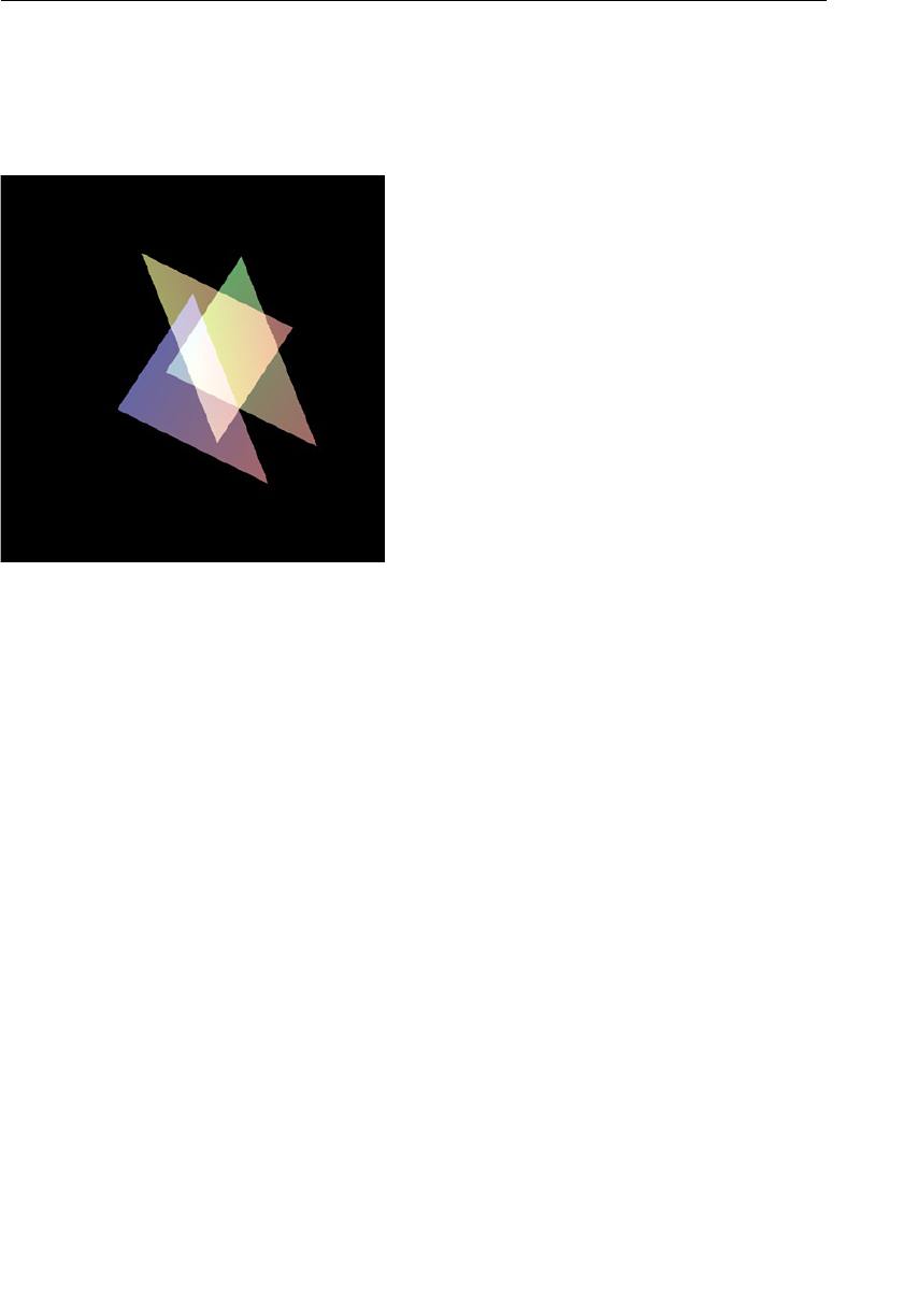
ptg11539634

Alpha Blending 381

Let’s add the code for steps 1 and 2, specify 0.4 as the alpha value of the color of the

triangles, and call the resulting program

LookAtBlendedTriangles . Figure 10.13 shows the

effect when run. As you can see, all triangles became semitransparent, and you are able to

see the triangles behind. When you move the eye point with the arrow key, you can see

that the blending is continuously taking place.

Figure 10.13 A screen shot of LookAtBlendedTriangles

Let’s look at the sample program.

Sample Program (LookAtBlendedTriangles.js)

LookAtBlendedTriangles.js is shown in Listing 10.9 . The code that has changed is in

lines 51 to 54, and the alpha value (0.4) is added to the definition of color information

initVertexBuffer() at lines 81 to 91. Accordingly, the size and stride parameters have

changed for

gl.vertexAttribPointer() .

Listing 10.9 LookAtBlenderTriangles.js

1 // LookAtBlendedTriangles.js

2 // LookAtTrianglesWithKey_ViewVolume.js is the original

…

25 function main() {

…

43 var n = initVertexBuffers(gl);

…

51 // Enable alpha blending

52 gl.enable (gl.BLEND);

53 // Set blending function

54 gl.blendFunc(gl.SRC_ALPHA, gl.ONE_MINUS_SRC_ALPHA);

…

ptg11539634

CHAPTER 10 Advanced Techniques

382

75 draw(gl, n, u_ViewMatrix, viewMatrix);

76 }

78 function initVertexBuffers(gl) {

79 var verticesColors = new Float32Array([

80 // Vertex coordinates and color(RGBA)

81 0.0, 0.5, -0.4, 0.4, 1.0, 0.4, 0.4 ,

82 -0.5, -0.5, -0.4, 0.4, 1.0, 0.4, 0.4 ,

…

91 0.5, -0.5, 0.0, 1.0, 0.4, 0.4, 0.4 ,

92 ]);

93 var n = 9;

…

127 return n;

128 }

Blending Function

Let’s explore the blending function gl.blendFunc() to understand how this can be used

to achieve the blending effect. You need two colors for blending: the color to blend

(source color) and the color to be blended (destination color). For example, when you

draw one triangle on top of the other, the color of the triangle already drawn is the desti-

nation color, and the color of the triangle drawn on top is the source color.

gl.blendFunc(src_factor, dst_factor)

Specify the method to blend the source color and the destination color. The blended

color is calculated as follows:

()

=×+ ×color RGB source color src_factor destination color dst_factor

Parameters src_factor Specifies the multiplier for the source color ( Table 10.2 ).

dst_factor Specifies the multiplier for the destination color ( Table

10.2 ).

Return value None

Errors INVALID_ENUM src_factor and dst_factor are none of the values in Table

10.2

Table 10.2 Constant Values that Can Be Specified as src_factor and dst_factor

Constant Multiplicand for R Multiplicand for G Multiplicand for B

gl.ZERO 0.0 0.0 0.0

gl.ONE 1.0 1.0 1.0

ptg11539634

Alpha Blending 383

Constant Multiplicand for R Multiplicand for G Multiplicand for B

gl.SRC_COLOR Rs Gs Bs

gl.ONE_MINUS_SRC_COLOR (1 – Rs) (1 – Gs) (1 – Bs)

gl.DST_COLOR Rd Gd Bd

gl.ONE_MINUS_DST_COLOR (1 – Rd) (1 – Bd) (1 – Gd)

gl.SRC_ALPHA As As As

gl.ONE_MINUS_SRC_ALPHA (1 – As) (1 – As) (1 – As)

gl.DST_ALPHA Ad Ad Ad

gl.ONE_MINUS_DST_ALPHA (1 – Ad) (1 – Ad) (1 – Ad)

gl.SRC_ALPHA_SATURATE min(As, Ad) min(As, Ad) min(As, Ad)

3 gl.CONSTANT_COLOR, gl.ONE_MINUSCONSTANT_COLOR, gl.CONSTANT_ALPHA , and gl.ONE_

MINUS_CONSTANT_ALPHA are removed from OpenGL.

(Rs,Gs,Bs,As) is the source color and (Rd,Gd,Bd,Ad) is the destination color.

In the sample program, you used the following:

54 gl.blendFunc(gl.SRC_ALPHA, gl.ONE_MINUS_SRC_ALPHA);

For example, if the source color is semitransparent green (0.0, 1.0, 0.0, 0.4) and the desti-

nation color is yellow (1.0, 1.0, 0.0, 1.0), src_factor becomes the alpha value 0.4 and dst_

factor becomes (1 – 0.4)=0.6. The calculation is shown in Figure 10.14 .

=)BGR(rolocrotcaf_tsd*rolocnoitanitsed+rotcaf_crs*rolocecruos

BGR

0.00.10.0rolocecruos

4.04.04.0rotcaf_crs

0.04.00.0

BGR

0.00.10.1rolocnoitanitsed

6.06.06.0rotcaf_tsd

0.06.06.0

0.00.16.0rolocdednelB

Figure 10.14 Calculation of gl.blendFunc(gl.SRC_ALPHA, gl.ONE_MINUS_SRC_ALPHA)

You can experiment with the other possible parameter values for src_factor , dst_factor , but

one that is often used is additive blending. When used, the result will become brighter

than the original value because it is a simple addition. It can be used for an indicator or

the lighting effect resulting from an explosion.

glBlendFunc(GL_SRC_ALPHA, GL_ONE);

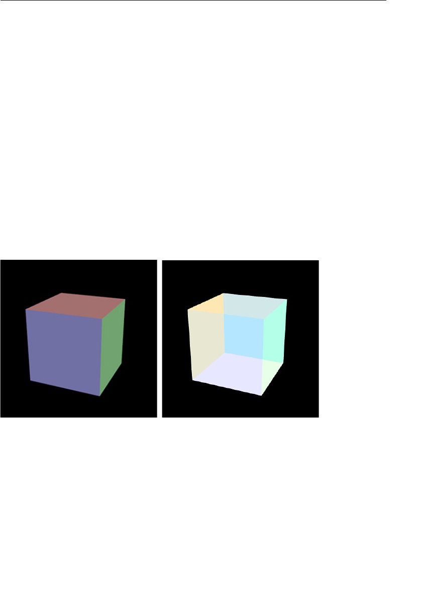
ptg11539634

CHAPTER 10 Advanced Techniques

384

Alpha Blend 3D Objects (BlendedCube.js)

Let’s now explore the effects of alpha blending on a representative 3D object, a cube, by

making it semitransparent. You will reuse the

ColoredCube sample program from Chapter

7 to create

BlendedCube , which adds the two steps needed for blending (see Listing 10.10 ).

Listing 10.10 BlendedCube.js

1 // BlendedCube.js

…

47 // Set the clear color and enable the depth test

48 gl.clearColor(0.0, 0.0, 0.0, 1.0);

49 gl.enable(gl.DEPTH_TEST);

50 // Enable alpha blending

51 gl.enable (gl.BLEND);

52 // Set blending function

53 gl.blendFunc(gl.SRC_ALPHA, gl.ONE_MINUS_SRC_ALPHA);

Unfortunately, if you run this program as-is, you won’t see the expected result (right side

of Figure 10.15 ); rather, you will see something similar to the left side, which is no differ-

ent from the original

ColoredCube used in Chapter 7 .

Figure 10.15 BlendedCube

This is because of the hidden surface removal function enabled at line 49. Blending only

takes place on the drawn surfaces. When the hidden surface removal function is enabled,

the hidden surfaces are not drawn, so there is no other surface to be blended with.

Therefore, you don’t see the blending effect as expected. To solve this problem, you can

simply comment out line 49 that enables the hidden surface removal function.

ptg11539634

Alpha Blending 385

48 gl.clearColor(0.0, 0.0, 0.0, 1.0);

49 // gl.enable(gl.DEPTH_TEST);

50 // Enable alpha blending

51 gl.enable (gl.BLEND);

How to Draw When Alpha Values Coexist

This is a quick solution, but it’s not very satisfactory because, as we’ve seen in Chapter 7 ,

hidden surface removal is often needed to correctly draw a 3D scene.

You can overcome this problem by drawing objects while turning the hidden surface

removal function on and off.

1. Enable the hidden surface removal function.

gl.enable(gl.DEPTH_TEST);

2. Draw all the opaque objects (whose alpha values are 1.0).

3. Make the depth buffer ( Chapter 7 ), which is used in the hidden surface removal,

read-only.

gl.depthMask(false);

4. Draw all the transparent objects (whose alpha values are smaller than 1.0). Note,

they should be sorted by the depth order and drawn back to front.

5. Make the depth buffer readable and writable.

gl.depthMask(true);

If you completely disable the hidden surface removal function, when there are transpar-

ent objects behind opaque objects, the transparent object will not be hidden behind the

opaque objects. So you need to control that with

gl.depthMask() . gl.depthMask() has the

following specification.

gl.depthMask(mask)

Enable or disable writing into the depth buffer.

Parameters mask Specifies whether the depth buffer is enabled for writing. If mask

false , depth buffer writing is disabled.

Return value None

Errors None

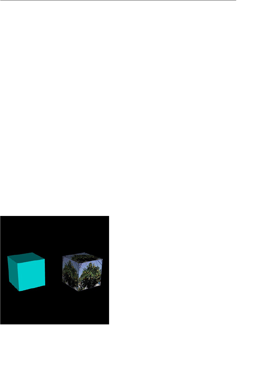
ptg11539634

CHAPTER 10 Advanced Techniques

386

The depth buffer was briefly introduced in Chapter 7 . The z values of fragments (which

are normalized to a value between 0.0 and 1.0) are written into the buffer. For example,

say there are two triangles on top of each other and you draw from the triangle on top.

First, the z value of the triangle on top is written into the depth buffer. Then, when the

triangle on bottom is drawn, the hidden surface removal function compares the z value

of its fragment that is going to be drawn, with the z value already written in the depth

buffer. Then only when the z value of the fragment that is going to be drawn is smaller

than the existing value in the buffer (that is, when it’s closer to the eye point) will the

fragment be drawn into the color buffer. This approach ensures that hidden surface

removal is achieved. Therefore, after drawing, the z value of the fragment of the surface

that can be seen from the eye point is left in the depth buffer.

Opaque objects are drawn into the color buffer in the correct order by removing the

hidden surfaces in the processing of steps 1 and 2, and the z value that represents the

order is written in the depth buffer. Transparent objects are drawn into the color buffer

using that z value in steps 3, 4, and 5, so the hidden surfaces of the transparent objects

behind the opaque objects will be removed. This results in the correct image being shown

where both objects coexist.

Switching Shaders

The sample programs in this book draw using a single vertex shader and a single fragment

shader. If all objects can be drawn with the same shaders, there is no problem. However,

if you want to change the drawing method for each object, you need to add significant

complexity to the shaders to achieve multiple effects. A solution is to prepare more than

one shader and then switch between these shaders as required. Here, you construct a

sample program,

ProgramObject , which draws a cube colored with a single color and

another cube with a texture image. Figure 10.16 shows a screen shot.

Figure 10.16 A screen shot of ProgramObject

ptg11539634

Switching Shaders 387

This program is also an example of the shading of an object with a texture image.

How to Implement Switching Shaders

The shaders can be switched easily by creating program objects, as explained in Chapter 8 ,

“Lighting Objects,” and switching them before drawing. Switching is carried out using the

function

gl.useProgram() . Because you are explicitly manipulating shader objects, you

cannot use the convenience function

initShaders() . However, you can use the function

createProgram() in cuon-utils.js , which is called from initShaders() .

The following is the processing flow of the sample program. It performs the same proce-

dure twice, so it looks long, but the essential code is simple:

1. Prepare the shaders to draw an object shaded with a single color.

2. Prepare the shaders to draw an object with a texture image.

3. Create a program object that has the shaders from step 1 with

createProgram() .

4. Create a program object that has the shaders from step 2 with createProgram() .

5. Specify the program object created by step 3 with gl.useProgram() .

6. Enable the buffer object after assigning it to the attribute variables.

7. Draw a cube (drawn in a single color).

8. Specify the program object created in step 4 using gl.useProgram() .

9. Enable the buffer object after assigning it to the attribute variables.

10. Draw a cube (texture is pasted).

Now let’s look at the sample program.

Sample Program (ProgramObject.js)

The key program code for steps 1 to 4 is shown in Listing 10.11 . Two types of vertex

shader and fragment shader are prepared:

SOLID_VSHADER_SOURCE (line 3) and SOLID_

FSHADER_SOURCE (line 19) to draw an object in a single color, and TEXTURE_VSHADER_SOURCE

(line 29) and

TEXTURE_FSHADER_SOURCE (line 46) to draw an object with a texture image.

Because the focus here is on how to switch the program objects, the contents of the

shaders are omitted.

Listing 10.11 ProgramObject (Process for Steps 1 to 4)

1 // ProgramObject.js

2 // Vertex shader for single color drawing <- (1)

3 var SOLID_VSHADER_SOURCE =

…

18 // Fragment shader for single color drawing

ptg11539634

CHAPTER 10 Advanced Techniques

388

19 var SOLID_FSHADER_SOURCE =

…

28 // Vertex shader for texture drawing <- (2)

29 var TEXTURE_VSHADER_SOURCE =

…

45 // Fragment shader for texture drawing

46 var TEXTURE_FSHADER_SOURCE =

…

58 function main() {

…

69 // Initialize shaders

70 var solidProgram = createProgram (gl, SOLID_VSHADER_SOURCE,

➥SOLID_FSHADER_SOURCE); <- (3)

71 var texProgram = createProgram (gl, TEXTURE_VSHADER_SOURCE,

➥TEXTURE_FSHADER_SOURCE); <- (4)

…

77 // Get the variables in the program object for single color drawing

78 solidProgram.a_Position = gl.getAttribLocation(solidProgram, ‘a_Position’);

79 solidProgram.a_Normal = gl.getAttribLocation(solidProgram, ‘a_Normal’);

…

83 // Get the storage location of attribute/uniform variables

84 texProgram.a_Position = gl.getAttribLocation(texProgram, ‘a_Position’);

85 texProgram.a_Normal = gl.getAttribLocation(texProgram, ‘a_Normal’);

…

89 texProgram.u_Sampler = gl.getUniformLocation(texProgram, ‘u_Sampler’);

…

99 // Set vertex information

100 var cube = initVertexBuffers(gl, solidProgram);

…

106 // Set texture

107 var texture = initTextures(gl, texProgram);

…

122 // Start drawing

123 var currentAngle = 0.0; // Current rotation angle (degrees)

124 var tick = function() {

125 currentAngle = animate(currentAngle); // Update rotation angle

…

128 // Draw a cube in single color

129 drawSolidCube(gl, solidProgram, cube, -2.0, currentAngle, viewProjMatrix);

130 // Draw a cube with texture

131 drawTexCube(gl, texProgram, cube, texture, 2.0, currentAngle,

➥viewProjMatrix);

132

133 window.requestAnimationFrame(tick, canvas);

ptg11539634

Switching Shaders 389

134 };

135 tick();

136 }

137

138 function initVertexBuffers(gl, program) {

…

148 var vertices = new Float32Array([ // Vertex coordinates

149 1.0, 1.0, 1.0, -1.0, 1.0, 1.0, -1.0,-1.0, 1.0, 1.0,-1.0, 1.0,

150 1.0, 1.0, 1.0, 1.0,-1.0, 1.0, 1.0,-1.0,-1.0, 1.0, 1.0,-1.0,

…

154 1.0,-1.0,-1.0, -1.0,-1.0,-1.0, -1.0, 1.0,-1.0, 1.0, 1.0,-1.0

155 ]);

156

157 var normals = new Float32Array([ // Normal

…

164 ]);

165

166 var texCoords = new Float32Array([ // Texture coordinates

…

173 ]);

174

175 var indices = new Uint8Array([ // Indices for vertices

…

182 ]);

183

184 var o = new Object(); // Use Object to return buffer objects

185

186 // Write vertex information to buffer object

187 o.vertexBuffer = initArrayBufferForLaterUse(gl, vertices, 3, gl.FLOAT);

188 o.normalBuffer = initArrayBufferForLaterUse(gl, normals, 3, gl.FLOAT);

189 o.texCoordBuffer = initArrayBufferForLaterUse(gl, texCoords, 2, gl.FLOAT);

190 o.indexBuffer = initElementArrayBufferForLaterUse(gl, indices,

➥gl.UNSIGNED_BYTE);

…

193 o.numIndices = indices.length;

…

199 return o;

200 }

Starting with the main() function in JavaScript, you first create a program object for

each shader with

createProgram() at lines 70 and 71. The arguments of the createPro-

gram() are the same as the initShaders() , and the return value is the program object.

You save each program object in

solidProgram and texProgram . Then you retrieve the

storage location of the attribute and uniform variables for each shader at lines 78 to 89.

You will store them in the corresponding properties of the program object, as you did in

ptg11539634

CHAPTER 10 Advanced Techniques

390

MultiJointModel_segment.js . Again, you leverage JavaScript’s ability to freely append a

new property of any type to an object.

The vertex information is then stored in the buffer object by

initVertexBuffers() at line

100. You need (1) vertex coordinates, (2) the normals, and (3) indices for the shader to

draw objects in a single color. In addition, for the shader to draw objects with a texture

image, you need the texture coordinates. The processing in

initVertexBuffers() handles

this and binds the correct buffer object to the corresponding attribute variables when the

program object is switched.

initVertexBuffers() prepares the vertex coordinates from line 148, normals from line

157, texture coordinates from line 166, and index arrays from line 175. Line 184 creates

object (

o ) of type Object . Then you store the buffer object to the property of the object

(lines 187 to 190). You can maintain each buffer object as a global variable, but that intro-

duces too many variables and makes it hard to understand the program. By using proper-

ties, you can more conveniently manage all four buffer objects using one object

You use initArrayBufferForLaterUse() , explained in MultiJointModel_segment.js , to

create each buffer object. This function writes vertex information into the buffer object

but does not assign it to the attribute variables. You use the buffer object name as its

property name to make it easier to understand. Line 199 returns the object

o as the return

value.

Once back in

main() in JavaScript, the texture image is set up in initTextures() at line

107, and then everything is ready to allow you to draw the two cube objects. First, you

draw a single color cube using

drawSolidCube() at line 129, and then you draw a cube

with a texture image by using

drawTexCube() at line 131. Listing 10.12 shows the latter

half of the steps, steps 5 through 10.

Listing 10.12 ProgramObject.js (Processes for Steps 5 through 10)

236 function drawSolidCube(gl, program, o, x, angle, viewProjMatrix) {

237 gl.useProgram(program); // Tell this program object is used <-(5)

238

239 // Assign the buffer objects and enable the assignment <-(6)

240 initAttributeVariable(gl, program.a_Position, o.vertexBuffer);

241 initAttributeVariable(gl, program.a_Normal, o.normalBuffer);

242 gl.bindBuffer(gl.ELEMENT_ARRAY_BUFFER, o.indexBuffer);

243

244 drawCube(gl, program, o, x, angle, viewProjMatrix); // Draw <-(7)

245 }

246

247 function drawTexCube(gl, program, o, texture, x, angle, viewProjMatrix) {

4 To keep the explanation simple, the object ( o ) was used. However, it is better programming practice

to create a new user-de ned type for managing the information about a buffer object and to use it to

manage the four buffers.

ptg11539634

Switching Shaders 391

248 gl.useProgram(program); // Tell this program object is used <-(8)

249

250 // Assign the buffer objects and enable the assignment <-(9)

251 initAttributeVariable(gl, program.a_Position, o.vertexBuffer);

252 initAttributeVariable(gl, program.a_Normal, o.normalBuffer);

253 initAttributeVariable(gl, program.a_TexCoord, o.texCoordBuffer);

254 gl.bindBuffer(gl.ELEMENT_ARRAY_BUFFER, o.indexBuffer);

255

256 // Bind texture object to texture unit 0

257 gl.activeTexture(gl.TEXTURE0);

258 gl.bindTexture(gl.TEXTURE_2D, texture);

259

260 drawCube(gl, program, o, x, angle, viewProjMatrix); // Draw <-(10)

261 }

262

263 // Assign the buffer objects and enable the assignment

264 function initAttributeVariable(gl, a_attribute, buffer) {

265 gl.bindBuffer(gl.ARRAY_BUFFER, buffer);

266 gl.vertexAttribPointer(a_attribute, buffer.num, buffer.type, false, 0, 0);

267 gl.enableVertexAttribArray(a_attribute);

268 }

…

275 function drawCube(gl, program, o, x, angle, viewProjMatrix) {

276 // Calculate a model matrix

…

281 // Calculate transformation matrix for normal

…

286 // Calculate a model view projection matrix

…

291 gl.drawElements(gl.TRIANGLES, o.numIndices, o.indexBuffer.type, 0);

292 }

drawSolidCube() is defined at line 236 and uses gl.useProgram() at line 237 to tell

the WebGL system that you will use the program (program object,

solidProgram )

specified by the argument. Then you can draw using

solidProgram . The buffer objects

for vertex coordinates and normals are assigned to attribute variables and enabled by

initAttributeVariable() at lines 240 and 241. This function is defined at line 264. Line

242 binds the buffer object for the indices to

gl.ELEMENT_ARRAY_BUFFER . With everything

set up, you then call

drawCube() at line 244, which uses gl.drawElements() at line 291 to

perform the draw operation.

drawTexCube() , defined at line 247, follows the same steps as drawSolidCube() . Line 253

is added to assign the buffer object for texture coordinates to the attribute variables, and

lines 257 and 258 are added to bind the texture object to the texture unit 0. The actual

drawing is performed in

drawCube() , just like drawSolidCube() .

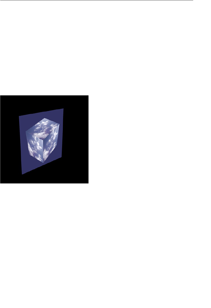
ptg11539634

CHAPTER 10 Advanced Techniques

392

Once you’ve mastered this basic technique, you can use it to switch between any number

of shader programs. This way you can use a variety of different drawing effects in a single

scene.

Use What You’ve Drawn as a Texture Image

One simple but powerful technique is to draw some 3D objects and then use the result-

ing image as a texture image for another 3D object. Essentially, if you can use the content

you’ve drawn as a texture image, you are able to generate images on-the-fly. This means

you do not need to download images from the network, and you can apply special effects

(such as motion blur and depth of field) before displaying the image. You can also use

this technique for shadowing, which will be explained in the next section. Here, you will

construct a sample program,

FramebufferObject , which maps a rotating cube drawn with

WebGL to a rectangle as a texture image. Figure 10.17 shows a screen shot.

Figure 10.17 FramebufferObject

If you actually run the program, you can see a rotating cube with a texture image of a

summer sky pasted to the rectangle as its texture. Significantly, the image of the cube that

is pasted on the rectangle is not a movie prepared in advance but a rotating cube drawn

by WebGL in real time. This is quite powerful, so let’s take a look at what WebGL must do

to achieve this.

Framebuffer Object and Renderbuffer Object

By default, the WebGL system draws using a color buffer and, when using the hidden

surface removal function, a depth buffer. The final image is kept in the color buffer.

The framebuffer object is an alternative mechanism you can use instead of a color buffer

or a depth buffer ( Figure 10.18 ). Unlike a color buffer, the content drawn in a framebuffer

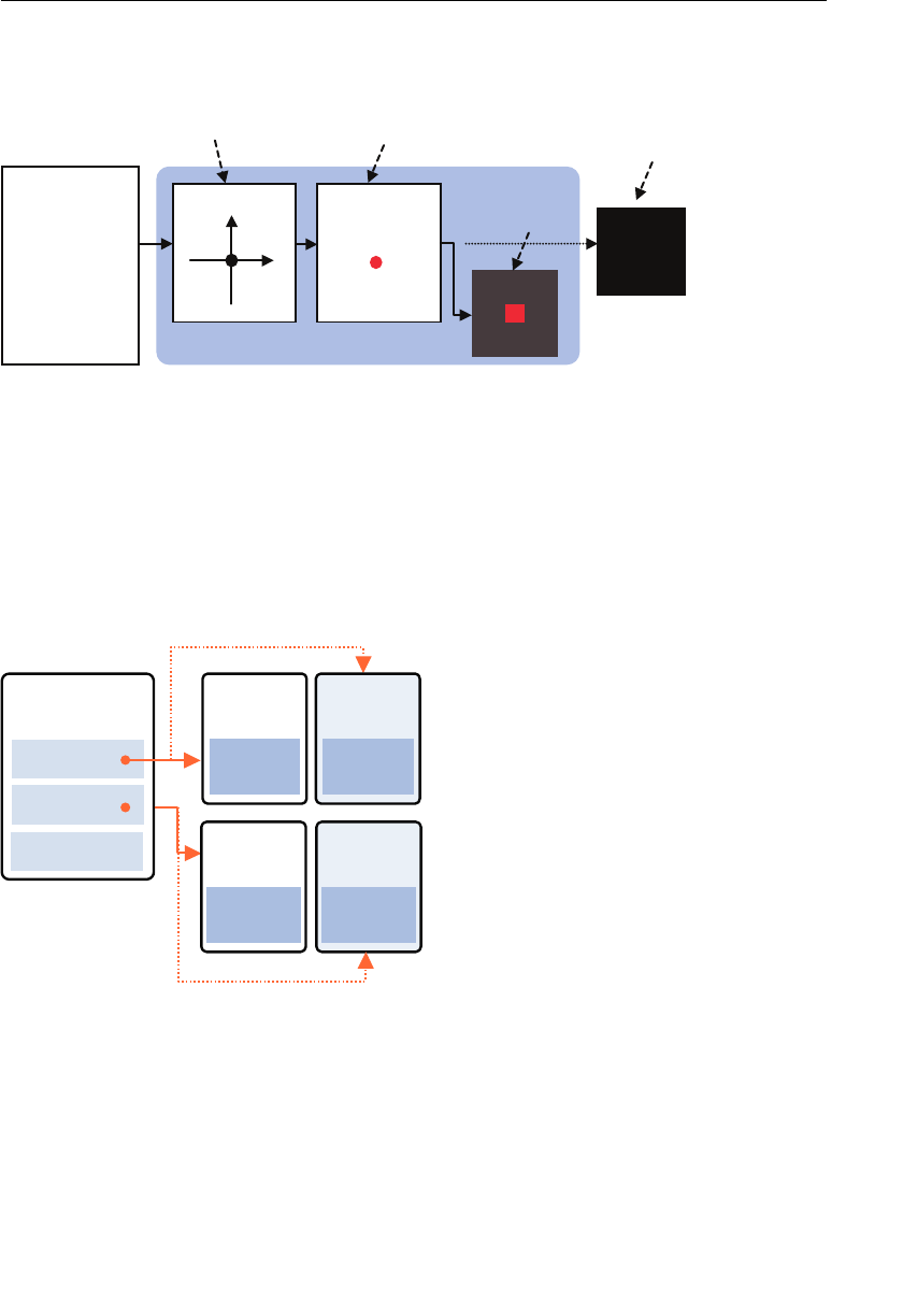
ptg11539634

Use What You’ve Drawn as a Texture Image 393

object is not directly displayed on the <canvas> . Therefore, you can use it if you want to

perform different types of processing before displaying the drawn content. Or you can use

it as a texture image. Such a technique is often referred to as offscreen drawing .

metsyS LGbeW

redahS xetreV tnemgarF

redahS

tpircSavaJ

{ )(niam noitcnuf

…LGbeWteg=lg rav

…

;)…(sredahStini

…

}

gnissecorp tnemgarf—repgnissecorp xetrev—rep

reffuB roloC

reffubemarF

tcejbO

Figure 10.18 Framebuffer object

The framebuffer object has the structure shown in Figure 10.19 and supports substitutes

for the color buffer and the depth buffer. As you can see, drawing is not carried out in

the framebuffer itself, but in the drawing areas of the objects that the framebuffer points

to. These objects are attached to the framebuffer using its attachment function. A color

attachment specifies the destination for drawing to be a replacement for the color buffer.

A depth attachment and a stencil attachment specify the replacements for the depth

buffer and stencil buffer.

reffubemarF

tcejbo

roloC

tnemhcatta

htpeD

tnemhcatta

licnetS

tnemhcatta

erutxeT

tcejbo

gniwarD

aera

erutxeT

tcejbo

gniwarD

aera

Render-

buffer

object

gniwarD

aera

Render-

buffer

object

gniwarD

aera

Figure 10.19 Framebuffer object, texture object, renderbuffer object

WebGL supports two types of objects that can be used to draw objects within: the texture

object that you saw in Chapter 5 , and the renderbuffer object . With the texture object,

the content drawn into the texture object can be used as a texture image. The render-

buffer object is a more general-purpose drawing area, allowing a variety of data types to

be written.

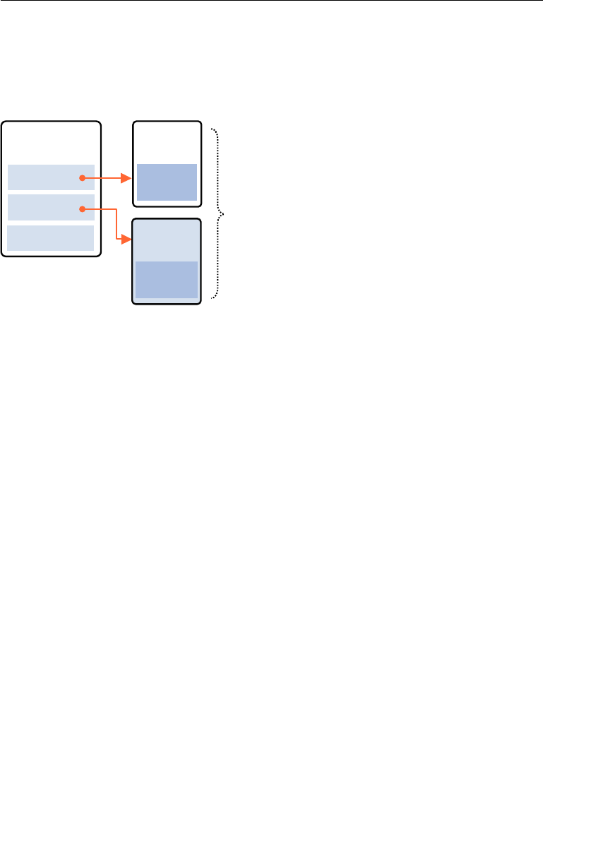
ptg11539634

CHAPTER 10 Advanced Techniques

394

How to Implement Using a Drawn Object as a Texture

When you want to use the content drawn into a framebuffer object as a texture object,

you actually need to use the content drawn into the color buffer for the texture object.

Because you also want to remove the hidden surfaces for drawing, you will set up the

framebuffer object as shown in Figure 10.20 .

reffubemarF

tcejbo

roloC

tnemhcatta

htpeD

tnemhcatta

licnetS

tnemhcatta

erutxeT

tcejbo

gniwarD

aera

gniwarD

aera

Render-

buffer

object

aeragniwardhcaefoezisehT

.lacitnediebtsum

Figure 10.20 Configuration of framebuffer object when using drawn content as a texture

The following eight steps are needed for realizing this configuration. These processes are

similar to the process for the buffer object. Step 2 was explained in Chapter 5 , so there are

essentially seven new processes:

1. Create a framebuffer object (

gl.createFramebuffer() ).

2. Create a texture object and set its size and parameters ( gl.createTexture() ,

gl.bindTexture() , gl.texImage2D() , gl.Parameteri() ).

3. Create a renderbuffer object ( gl.createRenderbuffer() ).

4. Bind the renderbuffer object to the target and set its size ( gl.bindRenderbuffer() ,

gl.renderbufferStorage() ).

5. Attach the texture object to the color attachment of the framebuffer object

(

gl.bindFramebuffer() , gl.framebufferTexture2D() ).

6. Attach the renderbuffer object to the depth attachment of the framebuffer object

(

gl.framebufferRenderbuffer() ).

7. Check whether the framebuffer object is configured correctly (

gl.checkFramebuffer-

Status() ).

8. Draw using the framebuffer object ( gl.bindFramebuffer() ).

Now let’s look at the sample program. The numbers in the sample program indicate the

code used to implement the steps.

ptg11539634

Use What You’ve Drawn as a Texture Image 395

Sample Program (FramebufferObjectj.js)

Steps 1 to 7 of FramebufferObject.js are shown in Listing 10.13 .

Listing 10.13 FramebufferObject.js (Processes for Steps 1 to 7)

1 // FramebufferObject.js

…

24 // Size of offscreen

25 var OFFSCREEN_WIDTH = 256;

26 var OFFSCREEN_HEIGHT = 256;

28 function main() {

…

55 // Set vertex information

56 var cube = initVertexBuffersForCube(gl);

57 var plane = initVertexBuffersForPlane(gl);

…

64 var texture = initTextures(gl);

…

70 // Initialize framebuffer object (FBO)

71 var fbo = initFramebufferObject(gl);

…

80 var viewProjMatrix = new Matrix4();/ For color buffer

81 viewProjMatrix.setPerspective(30, canvas.width/canvas.height, 1.0, 100.0);

82 viewProjMatrix.lookAt(0.0, 0.0, 7.0, 0.0, 0.0, 0.0, 0.0, 1.0, 0.0);

84 var viewProjMatrixFBO = new Matrix4(); // For FBO

85 viewProjMatrixFBO.setPerspective(30.0, OFFSCREEN_WIDTH/OFFSCREEN_HEIGHT,

➥1.0, 100.0);

86 viewProjMatrixFBO.lookAt(0.0, 2.0, 7.0, 0.0, 0.0, 0.0, 0.0, 1.0, 0.0);

…

92 draw(gl, canvas, fbo, plane, cube, currentAngle, texture, viewProjMatrix,

➥viewProjMatrixFBO);

…

96 }

…

263 function initFramebufferObject(gl) {

264 var framebuffer, texture, depthBuffer;

…

274 // Create a framebuffer object (FBO) <-(1)

275 framebuffer = gl.createFramebuffer();

…

281 // Create a texture object and set its size and parameters <-(2)

282 texture = gl.createTexture(); // Create a texture object

…

ptg11539634

CHAPTER 10 Advanced Techniques

396

287 gl.bindTexture(gl.TEXTURE_2D, texture);

288 gl.texImage2D(gl.TEXTURE_2D, 0, gl.RGBA, OFFSCREEN_WIDTH,

➥OFFSCREEN_HEIGHT, 0, gl.RGBA, gl.UNSIGNED_BYTE, null);

289 gl.texParameteri(gl.TEXTURE_2D, gl.TEXTURE_MIN_FILTER, gl.LINEAR);

290 framebuffer.texture = texture; // Store the texture object

291

292 // Create a renderbuffer object and set its size and parameters

293 depthBuffer = gl.createRenderbuffer(); // Create a renderbuffer <-(3)

…

298 gl.bindRenderbuffer(gl.RENDERBUFFER, depthBuffer); <-(4)

299 gl.renderbufferStorage(gl.RENDERBUFFER, gl.DEPTH_COMPONENT16,

➥OFFSCREEN_WIDTH, OFFSCREEN_HEIGHT);

300

301 // Attach the texture and the renderbuffer object to the FBO

302 gl.bindFramebuffer(gl.FRAMEBUFFER, framebuffer);

303 gl.framebufferTexture2D(gl.FRAMEBUFFER, gl.COLOR_ATTACHMENT0,

➥gl.TEXTURE_2D, texture, 0); <-(5)

304 gl.framebufferRenderbuffer(gl.FRAMEBUFFER, gl.DEPTH_ATTACHMENT,

➥gl.RENDERBUFFER, depthBuffer); <-(6)

305

306 // Check whether FBO is configured correctly <-(7)

307 var e = gl.checkFramebufferStatus(gl.FRAMEBUFFER);

308 if (e !== gl.FRAMEBUFFER_COMPLETE) {

309 console.log(‘Framebuffer object is incomplete: ‘ + e.toString());

310 return error();

311 }

312

…

319 return framebuffer;

320 }

The vertex shader and fragment shader are omitted because this sample program uses the

same shaders as

TexturedQuad.js in Chapter 5 , which pasted a texture image on a rect-

angle. The sample program in this section draws two objects: a cube and a rectangle. Just

as you did in

ProgramObject.js in the previous section, you assign multiple buffer objects

needed for drawing each object as properties of an

Object object. Then you store the

object to the variables

cube and plane . You will use them for drawing by assigning each

buffer in the object to the attribute variable.

The key point of this program is the initialization of the framebuffer object by

init-

FramebufferObject() at line 71. The initialized framebuffer object is stored in a variable

fbo and passed as the third argument of draw() at line 92. You’ll return to the function

draw() later. For now let’s examine initFramebufferObject() , at line 263, step by step.

This function performs steps 1 to 7. The view projection matrix for the framebuffer object

is prepared separately at line 84 because it is different from the one used for a color buffer.

ptg11539634

Use What You’ve Drawn as a Texture Image 397

Create Frame Buffer Object (gl.createFramebuffer())

You must create a framebuffer object before you can use it. The sample program creates it

at line 275:

275 framebuffer = gl.createFramebuffer();

You will use gl.createFramebuffer() to create the framebuffer object.

gl.createFramebuffer()

Create a framebuffer object.

Parameters None

Return value non-null The newly created framebuffer object.

null Failed to create a framebuffer object.

Errors None

You use

gl.deleteFramebuffer() to delete the created framebuffer object.

gl.deleteFramebuffer(framebuffer)

Delete a framebuffer object.

Parameters framebuffer Specifies the framebuffer object to be deleted.

Return value None

Errors None

Once you have created the framebuffer object, you need to attach a texture object to the

color attachment and a renderbuffer object to the depth attachment in the framebuffer

object. Let’s start by creating the texture object for the color attachment.

Create Texture Object and Set Its Size and Parameters

You have already seen how to create a texture object and set up its parameters

(

gl.TEXTURE_MIN_FILTER ) in Chapter 5 . You should note that its width and height are

OFFSCREEN_WIDTH and OFFSCREEN_HEIGHT , respectively. The size is smaller than that of the

<canvas> to make the drawing process faster.

282 texture = gl.createTexture(); // Create a texture object

…

287 gl.bindTexture(gl.TEXTURE_2D, texture);

ptg11539634

CHAPTER 10 Advanced Techniques

398

288 gl.texImage2D(gl.TEXTURE_2D, 0, gl.RGBA, OFFSCREEN_WIDTH, OFFSCREEN_HEIGHT, 0,

➥gl.RGBA, gl.UNSIGNED_BYTE, null );

289 gl.texParameteri(gl.TEXTURE_2D, gl.TEXTURE_MIN_FILTER, gl.LINEAR);

290 framebuffer.texture = texture; // Store the texture object

The gl.texImage2D() at line 288 allocates a drawing area in a texture object. You can allo-

cate a drawing area by specifying

null to the last argument, which is used to specify an

Image object. You will use this texture object later, so store it in framebuffer.texture at

line 290.

That completes the preparation for a texture object that is attached to the color attach-

ment. Next, you need to create a renderbuffer object for the depth buffer.

Create Renderbuffer Object (gl.createRenderbuffer())

Like texture buffers, you need to create a renderbuffer object before using it. The sample

program does this at line 293.

293 depthBuffer = gl.createRenderbuffer(); // Create a renderbuffer

You use gl.createRenderbuffer() to create the renderbuffer object.

gl.createRenderbuffer()

Create a renderbuffer object.

Parameters None

Return value Non-null The newly created renderbuffer object.

Null Failed to create a renderbuffer object.

Errors None

You use

gl.deleteRenderbuffer() to delete the created renderbuffer object.

gl.deleteRenderbuffer(renderbuffer)

Delete a renderbuffer object.

Parameters renderbuffer Specifies the renderbuffer object to be deleted.

Return value None

Errors None

ptg11539634

Use What You’ve Drawn as a Texture Image 399

The created renderbuffer object is used as a depth buffer here, so you store it in a variable

named

depthBuffer .

Bind Renderbuffer Object to Target and Set Size

(gl.bindRenderbuffer(), gl.renderbufferStorage())

When using the created renderbuffer object, you need to bind the renderbuffer object to a

target and perform the operation on that target.

298 gl.bindRenderbuffer(gl.RENDERBUFFER, depthBuffer);

299 gl.renderbufferStorage(gl.RENDERBUFFER, gl.DEPTH_COMPONENT16,

➥OFFSCREEN_WIDTH, OFFSCREEN_HEIGHT);

The renderbuffer object is bound to a target with gl.bindRenderbuffer() .

gl.bindRenderbuffer(target, renderbuffer)

Bind the renderbuffer object specified by renderbuffer to target . If null is specified as

renderbuffer , the renderbuffer is unbound from the target .

Parameters target Must be

gl.RENDERBUFFER.

renderbuffer Specifies the renderbuffer object.

Return value None

Errors INVALID_ENUM target is not

gl.RENDERBUFFER

When the binding is complete, you can set the format, width, and height of the render-

buffer object by using gl.renderbufferStorage() . You must set the same width and

height as the texture object that is used as the color attachment.

gl.renderbufferStorage(target, internalformat, width, height)

Create and initialize a renderbuffer object’s data store.

Parameters target Must be

gl.RENDERBUFFER.

internalformat Specifies the format of the renderbuffer.

gl.DEPTH_

COMPONENT16

The renderbuffer is used as a depth buffer.

gl.STENCIL_

INDEX8

The renderbuffer is used as a stencil buffer.

ptg11539634

CHAPTER 10 Advanced Techniques

400

gl.RGBA4 The renderbuffer is used as a color buffer. gl.RGBA4

(each RGBA component has 4, 4, 4, and 4 bits, respec-

tively),

gl.RGB5_A1 (each RGB component has 5 bits,

and A has 1 bit),

gl.RGB565 (each RGB component has

5, 6, and 5 bits, respectively)

gl.RGB5_A1

gl.RGB565

width, height Specifies the width and height of the renderbuffer in

pixels.

Return value None

Errors INVALID_ENUM Target is not

gl.RENDERBUFFER or internalformat is none

of the preceding values.

INVALID_OPERATION No renderbuffer is bound to target .

The preparations of the texture object and renderbuffer object of the framebuffer object

are now complete. At this stage, you can use the object for offscreen drawing.

Set Texture Object to Framebuffer Object (gl.bindFramebuffer(),

gl.framebufferTexture2D())

You use a framebuffer object in the same way you use a renderbuffer object: You need to

bind it to a target and operate on the target, not the framebuffer object itself.

302 gl.bindFramebuffer(gl.FRAMEBUFFER, framebuffer); // Bind to target

303 gl.framebufferTexture2D(gl.FRAMEBUFFER, gl.COLOR_ATTACHMENT0, gl.TEXTURE_2D,

➥texture, 0);

A framebuffer object is bound to a target with gl.bindFramebuffer() .

gl.bindFramebuffer(target, framebuffer)

Bind a framebuffer object to a target. If framebuffer is null , the binding is broken.

Parameters target Must be

gl.FRAMEBUFFER.

framebuffer Specify the framebuffer object.

Return value None

Errors INVALID_ENUM target is not

gl.FRAMEBUFFER

Once the framebuffer object is bound to target , you can use the target to write a texture

object to the framebuffer object. In this sample, you will use the texture object instead of

a color buffer so you attach the texture object to the color attachment of the framebuffer.

ptg11539634

Use What You’ve Drawn as a Texture Image 401

You can assign the texture object to the framebuffer object with gl.

framebufferTexture2D() .

gl.framebufferTexture2D(target, attachment, textarget, texture,

level)

Attach a texture object specified by texture to the framebuffer object bound by target.

Parameters target Must be

gl.FRAMEBUFFER .

attachment Specifies the attachment point of the framebuffer.

gl.COLOR_ATTACHMENT0 texture is used as a color buffer

gl.DEPTH_ATTACHMENT texture is used as a depth buffer

textarget Specifies the first argument of

gl.texImage2D()

(

gl.TEXTURE_2D or gl.CUBE_MAP_TEXTURE ).

texture Specifies a texture object to attach to the frame-

buffer attachment point.

level Specifies 0 (if you use a MIPMAP in texture , you

should specify its level).

Return value None

Errors INVALID_ENUM target is not

gl.FRAMEBUFFER . attachment

or textarget is none of the preceding values.

INVALID_VALUE level is not valid.

INVALID_OPERATION No framebuffer object is bound to target.

The 0 in the gl.COLOR_ATTACHMENT0 used for the attachment parameter is because a frame-

buffer object in OpenGL, the basis of WebGL, can hold multiple color attachments

(

gl.COLOR_ATTACHMENT0 , gl.COLOR_ATTACHMENT1 , gl.COLOR_ATTACHMENT2 …). However,

WebGL can use just one of them.

Once the color attachment has been attached to the framebuffer object, you need to

assign a renderbuffer object as a depth attachment. This follows a similar process.

Set Renderbuffer Object to Framebuffer Object

(gl.framebufferRenderbuffer())

You will use gl.framebufferRenderbuffer() to attach a renderbuffer object to a frame-

buffer object. You need a depth buffer because this sample program will remove hidden

surfaces. So the depth attachment needs to be attached.

ptg11539634

CHAPTER 10 Advanced Techniques

402

304 gl.framebufferRenderbuffer(gl.FRAMEBUFFER, gl.DEPTH_ATTACHMENT,

gl.RENDERBUFFER, depthBuffer);

gl.framebufferRenderbuffer(target, attachment, renderbuffertarget,

renderbuffer)

Attach a renderbuffer object specified by renderbuffer to the framebuffer object bound by

target.

Parameters target Must be

gl.FRAMEBUFFER .

attachment Specifies the attachment point of the framebuffer.

gl.COLOR_ATTACHMENT0 renderbuffer is used as a color buffer.

gl.DEPTH_ATTACHMENT renderbuffer is used as a depth buffer.

gl.STENCIL_ATTACHMENT renderbuffer is used as a stencil buffer.

renderbuffertarget Must be

gl.RENDERBUFFER.

renderbuffer Specifies a renderbuffer object to attach to the

framebuffer attachment point

Return value None

Errors INVALID_ENUM target is not a

gl.FRAMEBUFFER . attachment is

none of the above values. renderbuffertarget is

not

gl.RENDERBUFFER .

Now that you’ve completed the preparation of the color attachment and depth attach-

ment to the framebuffer object, you are ready to draw. But before that, let’s check that the

configuration of the framebuffer object is correct.

Check Configuration of Framebuffer Object

(gl.checkFramebufferStatus())

Obviously, when you use a framebuffer that is not correctly configured, an error occurs. As

you have seen in the past few sections, preparing a texture object and renderbuffer object

that are needed to configure the framebuffer object is a complex process that sometimes

generates mistakes. You can check whether the created framebuffer object is configured

correctly and is available with

gl.checkFramebufferStatus() .

307 var e = gl.checkFramebufferStatus(gl.FRAMEBUFFER); <- (7)

308 if (gl.FRAMEBUFFER_COMPLETE !== e) {

309 console.log(‘Frame buffer object is incomplete:’ + e.toString());

310 return error();

311 }

ptg11539634

Use What You’ve Drawn as a Texture Image 403

The following shows the specification of gl.checkFramebufferStatus() .

gl.checkFramebufferStatus(target)

Check the completeness status of a framebuffer bound to target.

Parameters target Must be

gl.FRAMEBUFFER.

Return value 0 Target is not

gl.FRAMEBUFFER.

Others

gl.FRAMEBUFFER_COMPLETE The framebuffer object is configured

correctly.

gl.FRAMEBUFFER_ INCOMPLETE_

ATTACHMENT

One of the framebuffer attachment points

is incomplete. (The attachment is not suffi-

cient. The texture object or the renderbuf-

fer object is invalid.)

gl.FRAMEBUFFER_ INCOMPLETE_

DIMENSIONS

The width or height of the texture object

or renderbuffer object of the attachment is

different.

gl.FRAMEBUFFER_ INCOMPLETE_

MISSING_ ATTACHMENT

The framebuffer does not have at least

one valid attachment.

Errors INVALID_ENUM target is not

gl.FRAMEBUFFER .

That completes the preparation of the framebuffer object. Let’s now take a look at the

draw() function.

Draw Using the Framebuffer Object

Listing 10.14 shows draw() . It switches the drawing destination to fbo (the framebuffer)

and draws a cube in the texture object. Then

drawTexturedPlane() uses the texture object

to draw a rectangle to the color buffer.

Listing 10.14 FramebufferObject.js (Process of (8))

321 function draw(gl, canvas, fbo, plane, cube, angle, texture, viewProjMatrix,

➥viewProjMatrixFBO) {

322 gl.bindFramebuffer(gl.FRAMEBUFFER, fbo); <-(8)

323 gl.viewport(0, 0, OFFSCREEN_WIDTH, OFFSCREEN_HEIGHT); // For FBO

324

325 gl.clearColor(0.2, 0.2, 0.4, 1.0); // Color is slightly changed

326 gl.clear(gl.COLOR_BUFFER_BIT | gl.DEPTH_BUFFER_BIT); // Clear FBO

ptg11539634

CHAPTER 10 Advanced Techniques

404

327 // Draw the cube

328 drawTexturedCube(gl, gl.program, cube, angle, texture, viewProjMatrixFBO);

329 // Change the drawing destination to color buffer

330 gl.bindFramebuffer(gl.FRAMEBUFFER, null);

331 // Set the size of view port back to that of

332 gl.viewport(0, 0, canvas.width, canvas.height);

333 gl.clearColor(0.0, 0.0, 0.0, 1.0);

334 gl.clear(gl.COLOR_BUFFER_BIT | gl.DEPTH_BUFFER_BIT);

335 // Draw the plane

336 drawTexturedPlane(gl, gl.program, plane, angle, fbo.texture , viewProjMatrix);

337 }

Line 322 switches the drawing destination to the framebuffer object using gl.bindFrame-

buffer() . As a result, draw operations using gl.drawArrays() or gl.drawElements() are

performed for the framebuffer object. Line 332 uses

gl.viewport() to specify the draw

area in the buffer (an offscreen area).

gl.viewport(x, y, width, height)

Set the viewport where

gl.drawArrays() or gl.drawElements() draws. In WebGL, x and

y are specified in the

<canvas> coordinate system.

Parameters x, y Specify the lower-left corner of the viewport rectangle (in

pixels).

width, height Specify the width and height of the viewport (in pixels).

Return value None

Errors None

Line 326 clears the texture image and the depth buffer bound to the framebuffer object.

When a cube is drawn at line 328, it is drawn in the texture image. To make it easier to

see the result, the clear color at line 325 is changed to a purplish blue from black. The

result of this is that the cube has been drawn into the texture buffer and is now available

for use as a texture image. The next step is to draw a rectangle (

plane ) using this texture

image. In this case, because you want to draw in the color buffer, you need to set the

drawing destination back to the color buffer. This is done at line 330 by specifying

null

for the second argument of

gl.bindFramebuffer() (that is, cancelling the binding). Then

line 336 draws the

plane . You should note that fbo.texture is passed as the texture argu-

ment and used to map the drawn content to the rectangle. You will notice that in this

sample program, the texture image is mapped onto the back side of the rectangle. This is

because WebGL, by default, draws both sides of a polygon. You can eliminate the back

face drawing by enabling the culling function using

gl.enable(gl.CULL_FACE) , which

increases the drawing speed (ideally making it twice as fast).

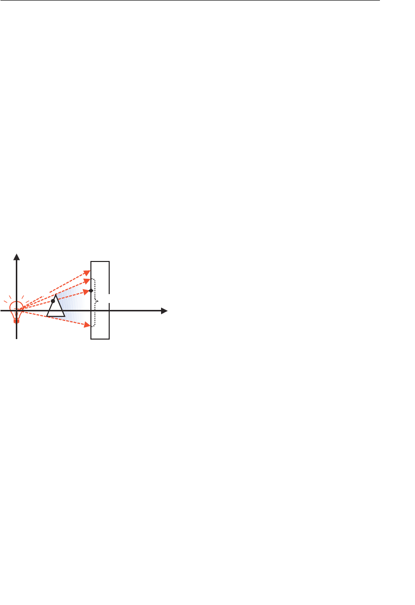
ptg11539634

Display Shadows 405

Display Shadows

Chapter 8 explained shading, which is one of the phenomena when light hits an object.

We briefly mentioned shadowing, another phenomena, but didn’t explain how to imple-

ment it. Let’s take a look at that now. There are several methods to realize shadowing,

but we will explain a method that uses a shadow map (depth map). This method is quite

expressive and used in a variety of computer graphics situations and even in special effects

in movies.

How to Implement Shadows

The shadow map method is based on the idea that the sun cannot see the shadow of

objects. Essentially, it works by considering the viewer’s eye point to be at the same posi-

tion as the light source and determining what can be seen from that point. All the objects

you can see would appear to be in the light. Anything behind those objects would be in

shadow. With this method, you can use the distance to the objects (in fact, you will use

the z value, which is the depth value) from the light source to judge whether the objects

are visible. As you can see in Figure 10.21 , where there are two points on the same line,

P1 and P2, P2 is in the shadow because the distance from the light source to P2 is longer

than P1.

1 p 2p

wodahsybdenekradaeraehT

Figure 10.21 Theory of shadow map

You need two pairs of shaders for this process: (1) a pair of shaders that calculate the

distance from the light source to the objects, and (2) a pair of shaders that draws the

shadow using the calculated distance. Then you need a method to pass the distance data

from the light source calculated in the first pair of shaders to the second pair of shaders.

You can use a texture image for this purpose. This texture image is called the shadow

map , so this method is called shadow mapping . The shadow mapping technique consists

of the following two processes:

1. Move the eye point to the position of the light source and draw objects from there.

Because the fragments drawn from the position are hit by the light, you write the

distances from the light source to each fragment in the texture image (shadow map).

2. Move the eye point back to the position from which you want to view the objects

and draw them from there. Compare the distance from the light source to the frag-

ments drawn in this step and the distance recorded in the shadow map from step

ptg11539634

CHAPTER 10 Advanced Techniques

406

1. If the former distance is greater, you can draw the fragment as in shadow (in the

darker color).

You will use the framebuffer object in step 1 to save the distance in the texture image.

Therefore, the configurations of the framebuffer object used here is the same as that of

FramebufferObject.js in Figure 10.20 . You also need to switch pairs of shaders between

steps 1 and 2 using the technique you learned in the section “Switching Shaders,” earlier

in this chapter. Now let’s take a look at the sample program

Shadow . Figure 10.22 shows

a screen shot where you can see a shadow of the red triangle cast onto the slanted white

rectangle.

Figure 10.22 Shadow

Sample Program (Shadow.js)

The key aspects of shadowing take place in the shaders, which are shown in Listing 10.15 .

Listing 10.15 Shadow.js (Shader part)

1 // Shadow.js

2 // Vertex shader program to generate a shadow map

3 var SHADOW_VSHADER_SOURCE =

…

6 ‘void main() {n’ +

7 ‘ gl_Position = u_MvpMatrix * a_Position;n’ +

8 ‘}n’;

10 // Fragment shader program for creating a shadow map

11 var SHADOW_FSHADER_SOURCE =

ptg11539634

Display Shadows 407

…

15 ‘void main() {n’ +

16 ‘ gl_FragColor = vec4(gl_FragCoord.z, 0.0, 0.0, 0.0);n’ + <-(1)

17 ‘}n’;

19 // Vertex shader program for regular drawing

20 var VSHADER_SOURCE =

…

23 ‘uniform mat4 u_MvpMatrix;n’ +

24 ‘uniform mat4 u_MvpMatrixFromLight;n’ +

25 ‘varying vec4 v_PositionFromLight;n’ +

26 ‘varying vec4 v_Color;n’ +

27 ‘void main() {n’ +

28 ‘ gl_Position = u_MvpMatrix * a_Position;n’ +

29 ‘ v_PositionFromLight = u_MvpMatrixFromLight * a_Position;n’ +

30 ‘ v_Color = a_Color;n’ +

31 ‘}n’;

33 // Fragment shader program for regular drawing

34 var FSHADER_SOURCE =

…

38 ‘uniform sampler2D u_ShadowMap;n’ +

39 ‘varying vec4 v_PositionFromLight;n’ +

40 ‘varying vec4 v_Color;n’ +

41 ‘void main() {n’ +

42 ‘ vec3 shadowCoord =(v_PositionFromLight.xyz/v_PositionFromLight.w)

➥/ 2.0 + 0.5;n’ +

43 ‘ vec4 rgbaDepth = texture2D(u_ShadowMap, shadowCoord.xy);n’ +

44 ‘ float depth = rgbaDepth.r;n’ + // Retrieve the z value from R

45 ‘ float visibility = (shadowCoord.z > depth + 0.005) ? 0.7:1.0;n’+ <-(2)

46 ‘ gl_FragColor = vec4(v_Color.rgb * visibility, v_Color.a);n’ +

47 ‘}n’;

Step 1 is performed in the shader responsible for the shadow map, defined from lines 3 to

17. You just switch the drawing destination to the framebuffer object, pass a model view

projection matrix in which an eye point is located at a light source to

u_MvpMatrix , and

draw the objects. This results in the distance from the light source to the fragments being

written into the texture map (shadow map) attached to the framebuffer object. The vertex

shader at line 7 just multiplies the model view projection matrix by the vertex coordinates

to calculate this distance. The fragment shader is more complex and needs to calculate the

distance from the light source to the drawn fragments. For this purpose, you can utilize

the built-in variable

gl_FragCoord of the fragment shader used in Chapter 5 .

gl_FragCoord is a vec4 type built-in variable that contains the coordinates of each frag-

ment.

gl_FragCoord.x and gl_FragCoord.y represents the position of the fragment on the

ptg11539634

CHAPTER 10 Advanced Techniques

408

screen, and gl_FragCoord.z contains the normalized z value in the range of [0, 1]. This is

calculated using (

gl_Position.z / gl.Position.w)/2.0+0.5. (See Section 2.12 of OpenGL ES

2.0 specification for further details.)

gl_FragCoord.z is specified in the range of 0.0 to 1.0,

with 0.0 representing the fragments on the near clipping plane and 1.0 representing those

on the far clipping plane. This value is written into the R (red) component value (any

component could be used) in the shadow map at line 16.

16 ‘ gl_FragColor = vec4(gl_FragCoord.z, 0.0, 0.0, 0.0);n’ + <-(1)

Subsequently, the z value for each fragment drawn from the eye point placed at the light

source is written into the shadow map. This shadow map is passed to

u_ShadowMap at

line 38.

For step 2, you need to draw the objects again after resetting the drawing destination

to the color buffer and moving the eye point to its original position. After drawing the

objects, you decide a fragment color by comparing the z value of the fragment with

that stored in the shadow map. This is done in the normal shaders from lines 20 to 47.

u_MvpMatrix is the model view projection matrix where the eye point is placed at the orig-

inal position and

uMvpMatrixFromLight , which was used to create the shadow map, is the

model view projection matrix where the eye point is moved to the light source. The main

task of the vertex shader defined at line 20 is calculating the coordinates of each fragment

from the light source and passing them to the fragment shader (line 29) to obtain the z

value of each fragment from the light source.

The fragment shader uses the coordinates to calculate the z value (line 42). As mentioned,

the shadow map contains the value of

(gl_Position.z/gl.Position.w)/2.0+0.5 . So

you could simply calculate the z value to compare with the value in the shadow map

(v_PositionFromLight.z/v_PositionFromLight.w)/2.0+0.5 . However, because you

need to get the texel value from the shadow map, line 42 performs the following extra

calculation using the same operation. To compare to the value in the shadow map, you

need to get the texel value from the shadow map whose texture coordinates correspond

to the coordinates (

v_PositionFromLight.x, v_PositionFromLight.y ). As you know,

v_PositionFromLight.x and v_PositionFromLight.y are the x and y coordinates in the

WebGL coordinate system (see Figure 2.18 in Chapter 2 ), and they range from –1.0 to 1.0.

On the other hand, the texture coordinates s and t in the shadow map range from 0.0 to

1.0 (see Figure 5.20 in Chapter 5 ). So, you need to convert the x and y coordinates to the s

and t coordinates. You can also do this with the same expression to calculate the z value.

That is:

The texture coordinate

s is (v_PositionFromLight.x/v_PositionFromLight.w)/2.0 + 0.5 .

The texture coordinate t is (v_PositionFromLight.y/v_PositionFromLight.w)/2.0 + 0.5 .

See also Section 2.12 of the OpenGL ES 2.0 specification

5 for further details about this calcu-

lation. These are carried out using the same type of calculation and can be achieved in

one line, as shown at line 42:

5 www.khronos.org/registry/gles/specs/2.0/es_full_spec_2.0.25.pdf

ptg11539634

Display Shadows 409

42 ‘ vec3 shadowCoord =(v_PositionFromLight.xyz/v_PositionFromLight.w)

➥/ 2.0 + 0.5;n’ +

43 ‘ vec4 rgbaDepth = texture2D(u_ShadowMap, shadowCoord.xy);n’ +

44 ‘ float depth = rgbaDepth.r;n’ + // Retrieve the z value from R

You retrieve the value from the shadow map at lines 43 and 44. Only the R value is

retrieved using

rgbaDepth.r at line 44 because you wrote it into the R component at line

16. Line 45 checks whether that fragment is in the shadow. When the position of the

fragment is determined to be greater than the depth (that is,

shadowCoord.z > depth) , a

value of 0.7 is stored in

visibility . The visibility is used at line 46 to draw the shadow

with a darker color:

45 ‘ float visibility = (shadowCoord.z > depth + 0.005) ? 0.7:1.0;n’+

46 ‘ gl_FragColor = vec4(v_Color.rgb * visibility, v_Color.a);n’ +

Line 45 adds a small offset of 0.005 to the depth value. To understand why this is needed,

try running the sample program without this number. You will see a striped pattern as

shown in Figure 10.23 , referred to as the Mach band .

Figure 10.23 Striped pattern

The value of 0.005 is added to suppress the stripe pattern. The stripe pattern occurs

because of the precision of the numbers you can store in the RGBA components. It’s a

little complex, but it’s worth understanding because this problem occurs elsewhere in 3D

graphics. The z value of the shadow map is stored in the R component of RGBA in the

texture map, which is an 8-bit number. This means that the precision of R is lower than

its comparison target (

shadowCoord.z ), which is of type float . For example, let the z value

simply be 0.1234567. If you represent the value using 8 bits, in other words using 256

ptg11539634

CHAPTER 10 Advanced Techniques

410

possibilities, you can represent the value in a precision of 1/256 (=0.0390625). So you can

represent 0.1234567 as follows:

0.1234567 / (1 / 256) = 31.6049152

Numbers below the decimal point cannot be used in 8 bits, so only 31 can be stored

in 8 bits. When you divide 31 by 256, you obtain 0.12109375 which, as you can see, is

smaller than the original value (0.1234567). This means that even if the fragment is at

the same position, its z value stored in the shadow map becomes smaller than its z value

shadowCoord.z . As a result, the z value in shadowCoord.z becomes larger than that in

the shadow map according to the position of the fragment resulting in the stripe patterns.

Because this happens because the precision of the R value is 1/256 (=0.00390625), by

adding a small offset, such as 0.005, to the R value, you can stop the stripe pattern from

appearing. Note that any offset greater than 1/256 will work; 0.005 was chosen because it

is 1/256 plus a small margin.

Next, let’s look at the JavaScript program that passes the data to the shader (see Listing

10.16 ) with a focus on the type of transformation matrices passed. To draw a shadow

clearly, the size of a texture map for the offscreen rendering defined at line 49 is larger

than that of the

<canvas> .

Listing 10.16 Shadow.js (JavaScript Part)

49 var OFFSCREEN_WIDTH = 1024, OFFSCREEN_HEIGHT = 1024;

50 var LIGHT_X = 0, LIGHT_Y = 7, LIGHT_Z = 2;

52 function main() {

…

63 // Initialize shaders for generating a shadow map

64 var shadowProgram = createProgram(gl, SHADOW_VSHADER_SOURCE,

➥SHADOW_FSHADER_SOURCE);

…

72 // Initialize shaders for regular drawing

73 var normalProgram = createProgram(gl, VSHADER_SOURCE, FSHADER_SOURCE);

…

85 // Set vertex information

86 var triangle = initVertexBuffersForTriangle(gl);

87 var plane = initVertexBuffersForPlane(gl);

…

93 // Initialize a framebuffer object (FBO)

94 var fbo = initFramebufferObject(gl);

…

99 gl.activeTexture(gl.TEXTURE0); // Set a texture object to the texture unit

100 gl.bindTexture(gl.TEXTURE_2D, fbo.texture);

…

106 var viewProjMatrixFromLight = new Matrix4(); // For the shadow map

ptg11539634

Display Shadows 411

107 viewProjMatrixFromLight.setPerspective(70.0,

➥OFFSCREEN_WIDTH/OFFSCREEN_HEIGHT, 1.0, 100.0);

108 viewProjMatrixFromLight.lookAt(LIGHT_X, LIGHT_Y, LIGHT_Z, 0.0, 0.0, 0.0, 0.0,

➥1.0, 0.0);

109

110 var viewProjMatrix = new Matrix4(); // For regular drawing

111 viewProjMatrix.setPerspective(45, canvas.width/canvas.height, 1.0, 100.0);

112 viewProjMatrix.lookAt(0.0, 7.0, 9.0, 0.0, 0.0, 0.0, 0.0, 1.0, 0.0);

113

114 var currentAngle = 0.0; // Current rotation angle [degrees]

115 var mvpMatrixFromLight_t = new Matrix4(); // For triangle

116 var mvpMatrixFromLight_p = new Matrix4(); // For plane

117 var tick = function() {

118 currentAngle = animate(currentAngle);

119 // Change the drawing destination to FBO

120 gl.bindFramebuffer(gl.FRAMEBUFFER, fbo);

…

124 gl.useProgram(shadowProgram); // For generating a shadow map

125 // Draw the triangle and the plane (for generating a shadow map)

126 drawTriangle(gl, shadowProgram, triangle, currentAngle,

➥viewProjMatrixFromLight);

127 mvpMatrixFromLight_t.set(g_mvpMatrix); // Used later

128 drawPlane(gl, shadowProgram, plane, viewProjMatrixFromLight);

129 mvpMatrixFromLight_p.set(g_mvpMatrix); // Used later

130 // Change the drawing destination to color buffer

131 gl.bindFramebuffer(gl.FRAMEBUFFER, null);

…

135 gl.useProgram(normalProgram); // For regular drawing

136 gl.uniform1i(normalProgram.u_ShadowMap, 0); // Pass gl.TEXTURE0

137 // Draw the triangle and plane (for regular drawing)

138 gl.uniformMatrix4fv(normalProgram.u_MvpMatrixFromLight, false,

➥mvpMatrixFromLight_t.elements);

139 drawTriangle(gl, normalProgram, triangle, currentAngle, viewProjMatrix);

140 gl.uniformMatrix4fv(normalProgram.u_MvpMatrixFromLight, false,

➥mvpMatrixFromLight_p.elements);

141 drawPlane(gl, normalProgram, plane, viewProjMatrix);

142

143 window.requestAnimationFrame(tick, canvas);

144 };

145 tick();

146 }

Let’s look at the main() function from line 52 in the JavaScript program. Line 64

initializes the shaders for generating the shadow map. Line 73 initializes the shaders

for normal drawing. Lines 86 and 87, which set up the vertex information and

ptg11539634

CHAPTER 10 Advanced Techniques

412

initFramebufferObject() at line 94, are the same as the FramebufferObject.js . Line 94

prepares a framebuffer object, which contains the texture object for a shadow map. Lines

99 and 100 enable texture unit 0 and bind it to the target. This texture unit is passed to

u_ShadowMap in the shaders for normal drawing.

Lines 106 to 108 prepare a view projection matrix to generate a shadow map. The key

point is that the first three arguments (that is, the position of an eye point) at line 108 are

specified as the position of the light source. Lines 110 to 112 prepare the view projection

matrix from the eye point where you want to view the scene.

Finally, you draw the triangle and plane using all the preceding information. First you

generate the shadow map, so you switch the drawing destination to the framebuffer

object at line 120. You draw the objects by using the shaders for generating a shadow map

(

shadowProgram ) at lines 126 and 128. You should note that lines 127 and 129 save the

model view projection matrices from the light source. Then the shadow map is generated,

and you use it to draw shadows with the code from line 135. Line 136 passes the map to

the fragment shader. Lines 138 and 140 pass the model view projection matrices saved at

line 127 and 129, respectively, to

u_MvpMatrixFromLight .

Increasing Precision

Although you’ve successfully calculated the shadow and drawn the scene with the shadow

included, the example code is only able to handle situations in which the light source is

close to the object. To see this, let’s change the y coordinate of the light source position

to 40:

50 var LIGHT_X = 0, LIGHT_Y = 40, LIGHT_Z = 2;

If you run the modified sample program, you can see that the shadow is not displayed—as

in the left side of Figure 10.24 . Obviously, you want the shadow to be displayed correctly,

as in the figure on the right.

The reason the shadow is no longer displayed when the distance from the light source to

the object is increased is that the value of

gl_FragCoord.z could not be stored in the R

component of the texture map because it has only an 8-bit precision. A simple solution to

this problem is to use not just the R component but the B, G, and A components. In other

words, you save the value separately in 4 bytes. There is a routine procedure to do this, so

let’s see the sample program. Only the fragment shader is changed.

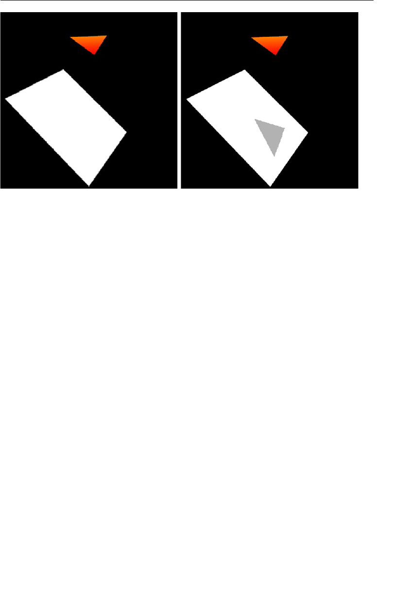
ptg11539634

Display Shadows 413

Sample Program (Shadow_highp.js)

Listing 10.17 shows the fragment shader of Shadow_highp.js . You can see that the

processing to handle the z value is more complex than that in

Shadow.js .

Listing 10.17 Shadow_highp.js

1 // Shadow_highp.js

…

10 // Fragment shader program for creating a shadow map

11 var SHADOW_FSHADER_SOURCE =

…

15 ‘void main() {n’ +

16 ‘ const vec4 bitShift = vec4(1.0, 256.0, 256.0 * 256.0, 256.0 * 256.0 *

➥256.0);n’ +

17 ‘ const vec4 bitMask = vec4(1.0/256.0, 1.0/256.0, 1.0/256.0, 0.0);n’ +

18 ‘ vec4 rgbaDepth = fract(gl_FragCoord.z * bitShift);n’ +

19 ‘ rgbaDepth -= rgbaDepth.gbaa * bitMask;n’ +

20 ‘ gl_FragColor = rgbaDepth;n’ +

21 ‘}n’;

…

37 // Fragment shader program for regular drawing

38 var FSHADER_SOURCE =

…

45 // Recalculate the z value from the rgba

46 ‘float unpackDepth(const in vec4 rgbaDepth) {n’ +

47 ‘ const vec4 bitShift = vec4(1.0, 1.0/256.0, 1.0/(256.0 * 256.0),

➥1.0/(256.0 * 256.0 * 256.0));n’ +

Figure 10.24 The shadow is not displayed

ptg11539634

CHAPTER 10 Advanced Techniques

414

48 ‘ float depth = dot(rgbaDepth, bitShift);n’ +

49 ‘ return depth;n’ +

50 ‘}n’ +

51 ‘void main() {n’ +

52 ‘ vec3 shadowCoord = (v_PositionFromLight.xyz /

➥v_PositionFromLight.w)/2.0 + 0.5;n’ +

53 ‘ vec4 rgbaDepth = texture2D(u_ShadowMap, shadowCoord.xy);n’ +

54 ‘ float depth = unpackDepth(rgbaDepth);n’ + // Recalculate the z

55 ‘ float visibility = (shadowCoord.z > depth + 0.0015)? 0.7:1.0;n’+

56 ‘ gl_FragColor = vec4(v_Color.rgb * visibility, v_Color.a);n’ +

57 ‘}n’;

The code that splits gl_FragCoord.z into 4 bytes (RGBA) is from lines 16 to 19. Because 1

byte can represent up to 1/256, you can store the value greater than 1/256 in R, the value

less than 1/256 and greater than 1/(256*256) in G, the value less than 1/(256*256) and

greater than 1/(256*256*256) in B, and the rest of value in A. Line 18 calculates each value

and stores it in the RGBA components, respectively. It can be written in one line using a

vec4 data type. The function fract() is a built-in one that discards numbers below the

decimal point for the value specified as its argument. Each value in

vec4 , calculated at

line 18, has more precision than 1 byte, so line 19 discards the value that does not fit in 1

byte. By substituting this result to

gl_FragColor at line 20, you can save the z value using

all four components of the RGBA type and achieve higher precision.

unpackDepth() at line 54 reads out the z value from the RGBA. This function is defined at

line 46. Line 48 performs the following calculation to convert the RGBA value to the origi-

nal z value. As you can see, the calculation is the same as the inner product, so you use

dot() at line 48.

()( )

=×+ +

×+××

depth rgbDepth r rgbaDepth g rgbaDepth b rgbaDepth a

. 1.0 .

256.0

256.0256.0

256.0256.0256.0

Now you have retrieved the distance (z value) successfully, so you just have to draw the

shadow by comparing the distance with

shadowCoord.z at line 55. In this case, 0.0015

is used as the value for adjusting the error (the stripe pattern), instead of 0.005. This is

because the precision of the z value stored in the shadow map is a

float type of medium

precision (that is, its precision is 2

–10 = 0.000976563, as shown in Table 6.15 in Chapter 6 ).

So you add a little margin to it and chose 0.0015 as the value. After that, the shadow can

be drawn correctly.

Load and Display 3D Models

In the previous chapters, you drew 3D objects by specifying their vertex coordinates

and color information by hand and stored them in arrays of type

Float32Array in

the JavaScript program. However, as mentioned earlier in the book, in most cases you

will actually read the vertex coordinates and color information from 3D model files

constructed by a 3D modeling tool.

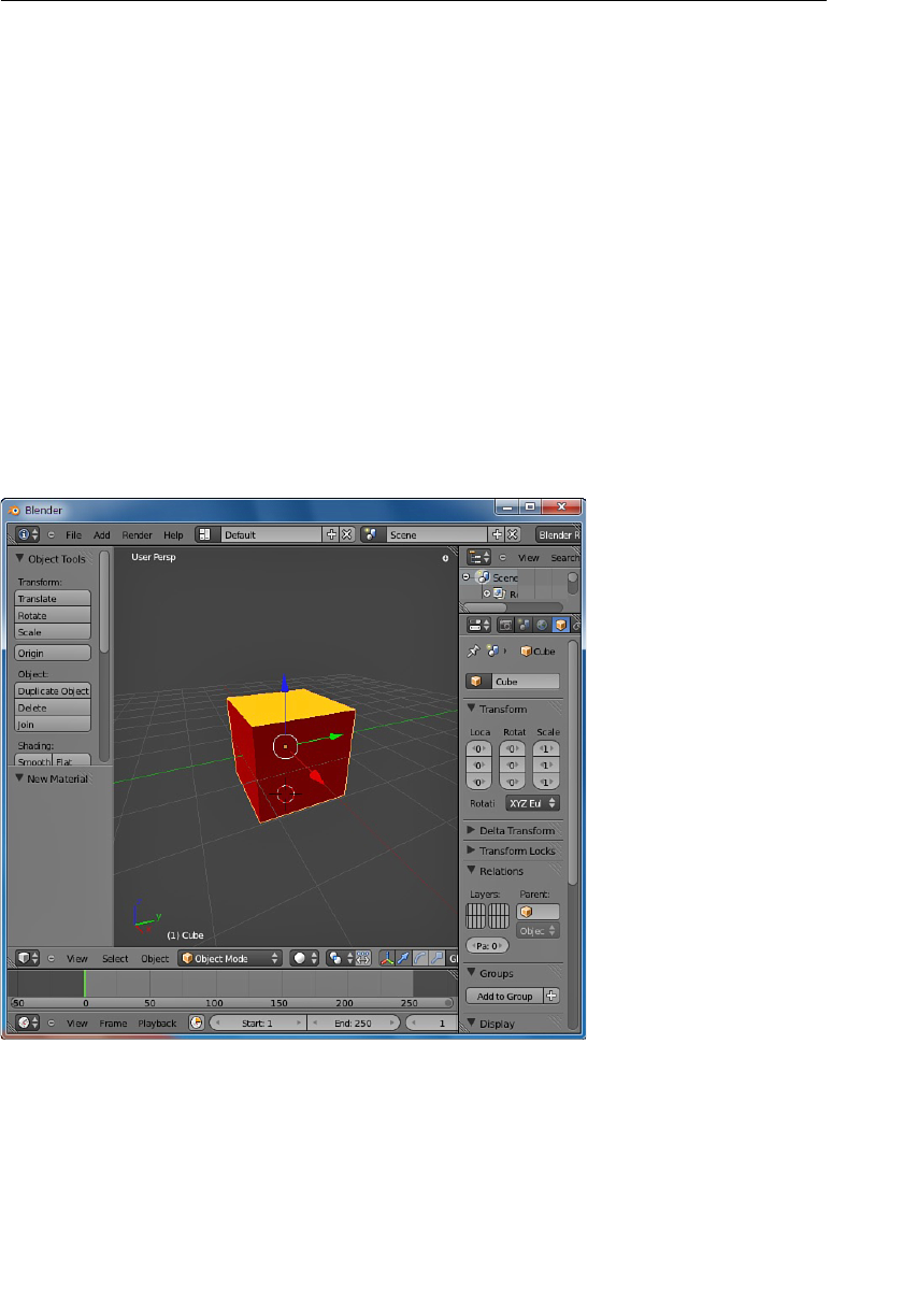
ptg11539634

Load and Display 3D Models 415

In this section, you construct a sample program that reads a 3D model constructed using

a 3D modeling tool. For this example, we use the Blender

6 modeling tool, which is a

popular tool with a free version available. Blender is able to export 3D model files using

the well-known OBJ format, which is text based and easy to read, understand, and parse.

OBJ is a geometry definition file format originally developed by Wavefront Technologies.

This file format is open and has been adopted by other 3D graphics vendors. Although

this means it is reasonably well known and used, it also means that there are a number

of variations in the format. To simplify the example code, we have made a number of

assumptions, such as not using textures. However, the example gives you a good under-

standing of how to read model data into your programs and provides a basis for you to

begin experimentation. The approach taken in the example code is designed to be reason-

ably generic and can be used for other text-based formats.

Start Blender and create a cube like that shown in Figure 10.25 . The color of one face of

this cube is orange, and the other faces are red. Then export the model to a file named

cube.obj . (You can find an example of it in the resources directory with the sample

programs.) Let’s take a look at

cube.obj , which, because it is a text file, can be opened

with a simple text editor.

Figure 10.25 Blender, 3D modeling tool

6. www.blender.org/

ptg11539634

CHAPTER 10 Advanced Techniques

416

Figure 10.26 shows the contents of cube.obj . Line numbers have been added to help with

the explanation and would not normally be in the file.

1 ‘‘ : e l i F J B O ) 0 b u s ( 0 6 . 2 v r e d n e l B #

2 g r o . r e d n e l b . w w w #

3 l t m . e b u c b i l l t m

4 e b u C o

5 0 0 0 0 0 0 . 1 — 0 0 0 0 0 0 . 1 — 0 0 0 0 0 0 . 1 v

6 0 0 0 0 0 0

. 1 0 0 0 0 0 0 . 1 — 0 0 0 0 0 0 . 1 v

7 0 0 0 0 0 0 . 1 0 0 0 0 0 0 . 1 — 0 0 0 0 0 0 . 1 — v

8 0 0 0 0 0 0 . 1 — 0 0 0 0 0 0 . 1 — 0 0 0 0 0 0 . 1 — v

9 0 0 0 0 0 0 . 1 — 0 0 0 0 0 0 . 1 0 0 0 0 0 0 . 1 v

0 1 0 0 0 0 0 . 1 0 0 0 0 0 0 . 1 0 0 0 0 0 0 . 1 v

1 0 0 0 0 0 0 . 1 0 0 0 0 0 0 . 1 0 0 0 0 0 0 . 1 — v

2 0 0 0 0 0 0 . 1 — 0 0 0 0 0 0 . 1 0 0 0 0 0 0 . 1 — v

3 l a i r e t a M l t m e s u

4 4

3 2 1 f

5 6 7 8 5 f

6 3 7 6 2 f

7 4 8 7 3 f

8 8 4 1 5 f

9 1 0 0 . l a i r e t a M l t m e s u

0 2 6 5 1 f

Figure 10.26 cube.obj

Once the model file has been created by the modeling tool, your program needs to read

the data and store it in the same type of data structures that you’ve used before. The

following steps are required:

1. Prepare the array (

vertices ) of type Float32Array and read the vertex coordinates of

the model from the file into the array.

2. Prepare the array (

colors ) of type Float32Array and read the colors of the model

from the file into the array.

3. Prepare the array (

normals ) of type Float32Array and read the normals of the model

form the file into the array.

4. Prepare the array (

indices ) of type Uint16Array (or Uint8Array ) and read the indices

of the vertices that specify the triangles that make up the model from the file into

the array.

5. Write the data read during steps 1 through 4 into the buffer object and then draw

the model using

gl.drawElements() .

So in this case, you read the data described in cube.obj (shown in Figure 10.26 ) in the

appropriate arrays and then draw the model in step 5. Reading data from the file requires

understanding the format of the file

cube.obj (referred to as the OBJ file).

ptg11539634

Load and Display 3D Models 417

The OBJ File Format

An OBJ file is made up of several sections,

7 including vertex positions, face definitions,

and material definitions. There may be multiple vertices, normals, and faces within their

sections:

• Lines beginning with a hash character (#) are comments. Lines 1 and 2 in Figure

10.26 are comments generated by Blender describing its version number and origin.

The remaining lines define the 3D model.

• Line 3 references an external materials file. The OBJ format maintains the material

information of the model in an external material file called an MTL file.

mtllib <external mtl filename>

specifies that the materials file is

cube.mtl .

• Line 4 specifies the named object in the following format:

This sample program does not use this information.

• Lines 5 to 12 define vertex positions in the following format using (x,y,z[,w]) coordi-

nates, where w is optional and defaults to 1.0.

v x y z [w]

In this example, it has eight vertices because the model is a standard cube.

• Lines 13 to 20 specify a material and the faces that use the material. Line 13 specifies

the material name, as defined in the MTL file referenced at line 4, and the specific

material using the following format:

usemtl <material name>

• The following lines, 14 to 18, define faces of the model and the material to be

applied to them. Faces are defined using lists of vertex, texture, and normal indices.

f v1 v2 v3 v4 …

v1, v2, v3, … are the vertex indices starting from 1 and matching the correspond-

ing vertex elements of a previously defined vertex list. This sample program handles

vertex and normals. Figure 10.26 does not contain normals, but if a face has a

normal, the following format would be used:

f v1 // vn1 v2 // vn2 v3 // vn3 …

vn1, vn2, vn3, … are the normal indices starting from 1.

7 See http://en.wikipedia.org/wiki/Wavefront_.obj_ le

ptg11539634

CHAPTER 10 Advanced Techniques

418

The MTL File Format

The MTL file may define multiple materials. Figure 10.27 shows cube.mtl .

‘ ‘ : e l i F L T M r e d n e l B # 1

2 : t n u o C l a i r e t a M #

l a i r e t a M l t m w e n

00 0 0 0 0 . 0 0 0 0 0 0 0 . 0 0 0 0 0 0 0 . 0 a K

00 0 0 0 0 . 0 0 0 0 0 0 0 . 0 0 0 0 0 0 0 .

1 d K

0 0 0 0 0 0 . 0 0 0 0 0 0 0 . 0 0 0 0 0 0 0 . 0 s K

1 3 4 8 7 0 . 6 9 s N

0 0 0 0 0 0 . 1 i N

0 0 0 0 0 0 . 1 d

0 m u l l i

0 1

1 0 0 . l a i r e t a M l t m w e n

1 1

0 0 0 0 0 0 . 0 0 0 0 0 0 0 . 0 0 0 0 0 0 0 . 0 a K

0 0 0 0 0 0 . 0 0 0 0 0 5 4 . 0 0 0 0 0 0 0 . 1 d K

2 1

3 1

0 0 0 0 0 0 . 0 0 0 0 0 0 0 . 0 0 0 0 0 0 0 . 0 s K

4 1

1 3 4 8 7 0 . 6 9 s N

5 1

0 0 0 0 0 0 . 1 i N

6 1

0 0 0 0 0 0 . 1 d

7 1

0 m u l l i 8 1

Figure 10.27 cube.mtl

• Lines 1 and 2 are comments that Blender generates.

• Each new material (from line 3) starts with the newmtl command:

newmtl <material name>

This is the material name that is used in the OBJ file.

• Lines 4 to 6 define the ambient, diffuse, and specular color using Ka , Kd , and Ks ,

respectively. Color definitions are in RGB format, where each component is between

0 and 1. This sample program uses only diffuse color.

• Line 7 specifies the weight of the specular color using Ns . Line 8 specifies the optical

density for the surface using

Ni . Line 9 specifies transparency using d . Line 10 speci-

fies illumination models using

illum . The sample program does not use this item of

information.

Given this understanding of the structure of the OBJ and MTL files, you have to extract

the vertex coordinates, colors, normals, and indices describing a face from the file, write

them into the buffer objects, and draw with

gl.drawElements() . The OBJ file may not

have the information on normals, but you can calculate them from the vertex coordinates

that make up a face by using a “cross product.”

Let’s look at the sample program.

8 If the vertices of a triangle are v0, v1, and v2, the vector of v0 and v1 is (x1, y1, z1), and the vector

of v1 and v2 is (x2, y2, z2), then the cross product is de ned as (y1*z2 – z1*y2, z1*x2 – x1*z2, x1*y2

– y1*z2). The result will be the normal for the triangle. (See the book 3D Math Primer for Graphics and

Game Development. )

ptg11539634

Load and Display 3D Models 419

Sample Program (OBJViewer.js)

The basic steps are as follows: (1) prepare an empty buffer object, (2) read an OBJ file (an

MTL file), (3) parse it, (4) write the results into the buffer object, and (5) draw. These steps

are implemented as shown in Listing 10.18 .

Listing 10.18 OBJViewer.js

1 // OBJViewer.js (

…

28 function main() {

…

40 if (!initShaders(gl, VSHADER_SOURCE, FSHADER_SOURCE)) {

41 console.log(‘Failed to initialize shaders.’);

42 return;

43 }

…

49 // Get the storage locations of attribute and uniform variables

50 var program = gl.program;

51 program.a_Position = gl.getAttribLocation(program, ‘a_Position’);

52 program.a_Normal = gl.getAttribLocation(program, ‘a_Normal’);

53 program.a_Color = gl.getAttribLocation(program, ‘a_Color’);

…

63 // Prepare empty buffer objects for vertex coordinates, colors, and normals

64 var model = initVertexBuffers(gl, program);

…

75 // Start reading the OBJ file

76 readOBJFile(‘../resources/cube.obj’, gl, model, 60, true);

…

81 draw(gl, gl.program, currentAngle, viewProjMatrix, model);

…

85 }

87 // Create a buffer object and perform the initial configuration

88 function initVertexBuffers(gl, program) {

89 var o = new Object();

90 o.vertexBuffer = createEmptyArrayBuffer(gl, program.a_Position, 3, gl.FLOAT);

91 o.normalBuffer = createEmptyArrayBuffer(gl, program.a_Normal, 3, gl.FLOAT);

92 o.colorBuffer = createEmptyArrayBuffer(gl, program.a_Color, 4, gl.FLOAT);

93 o.indexBuffer = gl.createBuffer();

…

98 return o;

99 }

100

101 // Create a buffer object, assign it to attribute variables, and enable the

➥assignment

ptg11539634

CHAPTER 10 Advanced Techniques

420

102 function createEmptyArrayBuffer(gl, a_attribute, num, type) {

103 var buffer = gl.createBuffer(); // Create a buffer object

…

108 gl.bindBuffer(gl.ARRAY_BUFFER, buffer);

109 gl.vertexAttribPointer(a_attribute, num, type, false, 0, 0);

110 gl.enableVertexAttribArray(a_attribute); // Enable the assignment

111

112 return buffer;

113 }

114

115 // Read a file

116 function readOBJFile(fileName, gl, model, scale, reverse) {

117 var request = new XMLHttpRequest();

118

119 request.onreadystatechange = function() {

120 if (request.readyState === 4 && request.status !== 404) {

121 onReadOBJFile(request.responseText, fileName, gl, model, scale, reverse);

122 }

123 }

124 request.open(‘GET’, fileName, true); // Create a request to get file

125 request.send(); // Send the request

126 }

127

128 var g_objDoc = null; // The information of OBJ file

129 var g_drawingInfo = null; // The information for drawing 3D model

130

131 // OBJ file has been read

132 function onReadOBJFile(fileString, fileName, gl, o, scale, reverse) {

133 var objDoc = new OBJDoc(fileName); // Create a OBJDoc object

134 var result = objDoc.parse(fileString, scale, reverse);

135 if (!result) {

136 g_objDoc = null; g_drawingInfo = null;

137 console.log(«OBJ file parsing error.»);

138 return;

139 }

140 g_objDoc = objDoc;

141 }

Within the JavaScript, the processing in initVertexBuffers() , called at line 64, has been

changed. The function simply prepares an empty buffer object for the vertex coordinates,

colors, and normals for the 3D model to be displayed. After parsing the OBJ file, the infor-

mation corresponding to each buffer object will be written in the object.

ptg11539634

Load and Display 3D Models 421

The initVertexBuffers() function at line 88 creates the appropriate empty buffer objects

at lines 90 to 92 using

createEmptyArrayBuffer() and assigns them to an attribute vari-

able. This function is defined at line 102 and, as you can see, creates a buffer object

(line 103), assigns it to an attribute variable (line 109), and enables the assignment (line

110), but it does not write the data. After storing these buffer objects to

model at line

64, the preparations of the buffer object are completed. The next step is to read the OBJ

file contents into this buffer, which takes place at line 76 using

readOBJFile() . The first

argument is the location of the file (URL), the second one is

gl , and the third one is the

Object object ( model ) that packages the buffer objects. The tasks carried out by this func-

tion are similar to those when loading a texture image using the

Image object and are

shown here:

(2.1) Create an

XMLHttpRequest object (line 117).

(2.2) Register the event handler to be called when the loading of the file is completed

(line 119).

(2.3) Create a request to acquire the file using the

open() method (line 124).

(2.4) Send the request to acquire the file (line 125).

Line 117 creates the XMLHttpRequest object, which sends an HTTP request to a web server.

Line 119 is the registration of the event handler that will be called after the browser has

loaded the file. Line 124 creates the request to acquire the file using the

open() method.

Because you are requesting a file, the first argument is

GET , and the second one is the URL

for the file. The last one specifies whether or not the request is asynchronous. Finally, line

125 uses the

send() method to send the request to the web server to get the file.

Once the browser has loaded the file, the event handler at line 119 is called. Line 120

checks for any errors returned by the load request. If the

readyState property is 4, it indi-

cates that the loading process is completed. However, if the

readyState is not 4 and the

status property is 404, it indicates that the specified file does not exist. The 404 error

is the same as “404 Not Found,” which is displayed when you try to display a web page

that does not exist. When the file has been loaded successfully,

onReadOBJFile() is called,

which is defined at line 132 and takes five arguments. The first argument,

responseText ,

contains the contents of the loaded file as one string. An

OBJDoc object is created at line

133, which will be used, via the

parse() method, to extract the results in a form that

WebGL can easily use. The details will be explained next. Line 140 assigns the

objDoc ,

which contains the parsing result in

g_objDoc for rendering the model later.

9 Note: When you want to run the sample programs that use external  les in Chrome from your

local disk, you should add the option —allow-file-access-from-files to Chrome. This is for

security reasons. Chrome, by default, does not allow access to local  les such as ../resources/

cube.obj . For Firefox, the equivalent parameter, set via account:config , is security.fileuri.

strict_origin_policy , which should be set to false . Remember to set it back as you open a

security loophole if local  le access is enabled.

ptg11539634

CHAPTER 10 Advanced Techniques

422

User-Defined Object

Before proceeding to the explanation of the remaining code of OBJViewer.js , you need to

understand how to create your own (user-defined) objects in JavaScript.

OBJViewer.js uses

user-defined objects to parse an OBJ file. In JavaScript, you can create user-defined objects

which, once created, are treated in the same way as built-in objects like

Array and Date .

The following is the StringParser object used in OBJViewer.js . The key aspects are how

to define a constructor to create a user-defined object and how to add methods to the

object. The constructor is a special method that is called when creating an object with

new . The following is the constructor for the StringParser object:

595 // Constructor

596 var StringParser = function(str) {

597 this.str; // Store the string specified by the argument

598 this.index; // Position in the string to be processed

599 this.init(str);

600 }

You can define the constructor with the anonymous function (see Chapter 2 ). Its param-

eter is the one that will be specified when creating the object with

new . Lines 597 and

598 are the declaration of properties that can be used for this new object type, similar to

properties like the length property of Array. You can define the property by writing the

keyword

this followed by . and the property name. Line 599 then calls init() , an initial-

ization method that has been defined for this user-defined object.

Let’s take a look at

init() . You can add a method to the object by writing the method

name after the keyword

prototype . The body of the method is also defined using an

anonymous function:

601 // Initialize StringParser object

602 StringParser.prototype.init = function(str) {

603 this.str = str;

604 this.index = 0;

605 }

What is convenient here is that you can access the property that is defined in the

constructor from the method. The

this.str at line 603 refers to this.str defined at line

597 in the constructor. The

this.index at line 604 refers to this.index at line 598 in the

constructor. Let’s try using this

StringParse object:

ptg11539634

Load and Display 3D Models 423

var sp = new StringParser(‘Tomorrow is another day.’);

alert(sp.str); // «Tomorrow is another day.» is displayed.

sp.str = ‘Quo Vadis’; // The content of str is changed to «Quo Vadis».

alert(sp.str); // «Quo Vadis» is displayed

sp.init(‘Cinderella, tonight?’);

alert(sp.str); // «Cinderella, tonight?» is displayed

Let’s look at another method, skipDelimiters() , that skips the delimiters (tab, space, (, ),

or ”) in a string:

608 StringParser.prototype.skipDelimiters = function() {

609 for(var i = this.index, len = this.str.length; i < len; i++) {

610 var c = this.str.charAt(i);

611 // Skip TAB, Space, (, ), and «

612 if (c == ‘t’|| c == ‘ ‘ || c == ‘(‘ || c == ‘)’ || c == ‘»‘) continue;

613 break;

614 }

615 this.index = i;

616 }

The charAt() method at line 610 is supported by the String object that manages a string

and retrieves the character specified by the argument from the string.

Now let’s look at the parser code in

OBJViewer.js .

Sample Program (Parser Code in OBJViewer.js)

OBJViewer.js parses the content of an OBJ file line by line and converts it to the structure

shown in Figure 10.28 . Each box in Figure 10.28 is a user-defined object. Although the

parser code in

OBJViewer.js looks quite complex, the core parsing process is simple. The

complexity comes because it is repeated several times. Let’s take a look at the core process-

ing, which once you understand will allow you to understand the whole process.

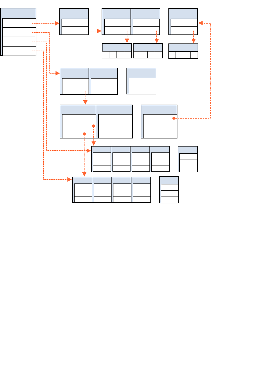
ptg11539634

424 CHAPTER 10 Advanced Techniques

tcejbOJBO tcejbOJBO

xetreV

coDJBO

sltm

stcejbo

slamron

secitrev

tcejbOJBO

eman

secaf

coDLTM

etelpmoc

slairetam

lairetaM

eman

roloc

roloC

lairetaM

eman

roloc

roloC

lairetaM

eman

roloc

roloC

…

eman

secaf

eman

secaf

…

ecaF

emaNlairetam

secidnIv

secidnIn

ecaF

emaNlairetam

secidnIv

secidnIn

ecaF

emaNlairetam

secidnIv

secidnIn

…

xetreV

…

lamroN lamroN lamroN lamroN lamroN

rgba rgba rgba

Figure 10.28 The internal structure after parsing an OBJ file

Listing 10.19 shows the basic code of

OBJViewer.js .

Listing 10.19 OBJViewer.js (Parser Part)

214 // OBJDoc object

215 // Constructor

216 var OBJDoc = function(fileName) {

217 this.fileName = fileName;

218 this.mtls = new Array(0); // Initialize the property for MTL

219 this.objects = new Array(0); // Initialize the property for Object

220 this.vertices = new Array(0); // Initialize the property for Vertex

221 this.normals = new Array(0); // Initialize the property for Normal

222 }

223

224 // Parsing the OBJ file

225 OBJDoc.prototype.parse = function(fileString, scale, reverseNormal) {

ptg11539634

Load and Display 3D Models 425

226 var lines = fileString.split(‘n’); // Break up into lines

227 lines.push(null); // Append null

228 var index = 0; // Initialize index of line

229

230 var currentObject = null;

231 var currentMaterialName = «»;

232

233 // Parse line by line

234 var line; // A string in the line to be parsed

235 var sp = new StringParser(); // Create StringParser

236 while ((line = lines[index++]) != null) {

237 sp.init(line); // init StringParser

238 var command = sp.getWord(); // Get command

239 if(command == null) continue; // check null command

240

241 switch(command){

242 case ‘#’:

243 continue; // Skip comments

244 case ‘mtllib’: // Read Material chunk

245 var path = this.parseMtllib(sp, this.fileName);

246 var mtl = new MTLDoc(); // Create MTL instance

247 this.mtls.push(mtl);

248 var request = new XMLHttpRequest();

249 request.onreadystatechange = function() {

250 if (request.readyState == 4) {

251 if (request.status != 404) {

252 onReadMTLFile(request.responseText, mtl);

253 }else{

254 mtl.complete = true;

255 }

256 }

257 }

258 request.open(‘GET’, path, true); // Create a request to get file

259 request.send(); // Send the request

260 continue; // Go to the next line

261 case ‘o’:

262 case ‘g’: // Read Object name

263 var object = this.parseObjectName(sp);

264 this.objects.push(object);

265 currentObject = object;

266 continue; // Go to the next line

267 case ‘v’: // Read vertex

268 var vertex = this.parseVertex(sp, scale);

269 this.vertices.push(vertex);

270 continue; // Go to the next line

ptg11539634

CHAPTER 10 Advanced Techniques

426

271 case ‘vn’: // Read normal

272 var normal = this.parseNormal(sp);

273 this.normals.push(normal);

274 continue; // Go to the next line

275 case ‘usemtl’: // Read Material name

276 currentMaterialName = this.parseUsemtl(sp);

277 continue; // Go to the next line

278 case ‘f’: // Read face

279 var face = this.parseFace(sp, currentMaterialName, this.vertices,

➥reverse);

280 currentObject.addFace(face);

281 continue; // Go to the next line

282 }

283 }

284

285 return true;

286 }

Lines 216 to 222 define the constructor for the OBJDoc object, which consists of five prop-

erties that will be parsed and set up. The actual parsing is done in the

parse() method at

line 225. The content of the OBJ file is passed as one string to the argument fileString of

the

parse() method and then split into manageable pieces using the split() method.

This method splits a string into pieces delimited by the characters specified as the argu-

ment. As you can see at line 226, the argument specifies “n” (new line), so each line is

stored in

this.line s as an array. null is appended at the end of the array at line 227 to

make it easy to find the end of the array.

this.index indicates how many lines have been

parsed and is initialized to 0 at line 228.

You have already seen the

StringParser object, which is created at line 235, in the previ-

ous section. This object is used for parsing the content of the line.

Now you are ready to start parsing the OBJ file. Each line is stored in

line using this.

lines[this.index++] at line 236. Line 237 writes the line to sp ( StringParser ). Line 238

gets the first word of the line using

sp.getWord() and stores it in command . You use the

methods shown in Table 10.3 , where “word” in the table indicates a string surrounded by

a delimiter (tab, space, (, ), or ”).

Table 10.3 Method that StringParser Supports

Method Description

StringParser.init(str) Initialize StringParser to be able to parse str.

StringParser.getWord() Get a word.

StringParser.skipToNext-

Word()

Skip to the beginning of the next word.

ptg11539634

Load and Display 3D Models 427

Method Description

StringParser.getInt() Get a word and convert it to an integer number.

StringParser.getFloat() Get a word and convert it to a floating point number.

The

switch statement at line 241 checks the command to determine how to process the

following lines in the OBJ file.

If the command is

# (line 242), the line is a comment. Line 243 skips it using continue .

If the command is mtllib (line 241), the line is a reference to an MTL file. Line 245 gener-

ates the path to the file. Line 246 creates an MTLDoc object for storing the material infor-

mation in the MTL file, and line 247 stores it in

this.mtls . Then lines 248 to 259 read the

file in the same way that you read an OBJ file. The MTL file is parsed by

onReadMTLfile() ,

which is called when it is loaded.

If the command is

o (line 261) or g (line 262), it indicates a named object or group. Line

263 parses the line and returns the results in

OBJObject . This object is stored in this.

objects at line 264 and currentObject .

If the command is v , the line is a vertex position. Line 268 parses (x, y, z) and returns the

result in

Vertex object. This object is stored in this.vertices at line 269.

If the command is f , it indicates that the line is a face definition. Line 279 parses it and

returns the result in the

Face object. This object is stored in the currentObject . Let’s take

a look at

parseVertex() , which is shown in Listing 10.20 .

Listing 10.20 OBJViewer.js (parseVertex())

302 OBJDoc.prototype.parseVertex = function(sp, scale) {

303 var x = sp.getFloat() * scale;

304 var y = sp.getFloat() * scale;

305 var z = sp.getFloat() * scale;

306 return (new Vertex(x, y, z));

307 }

Line 303 retrieves the x value from the line using sp.getFloat() . A scaling factor is

applied when the model is too small or large. After retrieving the three coordinates, line

306 creates a

Vertex object using x, y, and z and returns it.

Once the OBJ file and MTL files have been fully parsed, the arrays for the vertex coordi-

nates, colors, normals, and indices are created from the structure shown in Figure 10.28 .

Then

onReadComplete() is called to write them into the buffer object (see Listing 10.21 ).

ptg11539634

CHAPTER 10 Advanced Techniques

428

Listing 10.21 OBJViewer.js (onReadComplete())

176 // OBJ File has been read completely

177 function onReadComplete(gl, model, objDoc) {

178 // Acquire the vertex coordinates and colors from OBJ file

179 var drawingInfo = objDoc.getDrawingInfo();

180

181 // Write date into the buffer object

182 gl.bindBuffer(gl.ARRAY_BUFFER, model.vertexBuffer);

183 gl.bufferData(gl.ARRAY_BUFFER, drawingInfo.vertices,gl.STATIC_DRAW);

184

185 gl.bindBuffer(gl.ARRAY_BUFFER, model.normalBuffer);

186 gl.bufferData(gl.ARRAY_BUFFER, drawingInfo.normals, gl.STATIC_DRAW);

187

188 gl.bindBuffer(gl.ARRAY_BUFFER, model.colorBuffer);

189 gl.bufferData(gl.ARRAY_BUFFER, drawingInfo.colors, gl.STATIC_DRAW);

190

191 // Write the indices to the buffer object

192 gl.bindBuffer(gl.ELEMENT_ARRAY_BUFFER, model.indexBuffer);

193 gl.bufferData(gl.ELEMENT_ARRAY_BUFFER, drawingInfo.indices, gl.STATIC_DRAW);

194

195 return drawingInfo;

196 }

This method is straightforward and starts at Line 178, which retrieves the drawing infor-

mation from

objDoc that contains the results from parsing the OBJ file. Lines 183, 186,

189, and 193 write vertices, normals, colors, and indices into the respective buffer objects.

The function

getDrawingInfo() at line 451 retrieves the vertices, normals, colors, and

indices from the

objDoc and is shown in Listing 10.22 .

Listing 10.22 OBJViewer.js (Retrieving the Drawing Information)

450 // Retrieve the information for drawing 3D model

451 OBJDoc.prototype.getDrawingInfo = function() {

452 // Create an array for vertex coordinates, normals, colors, and indices

453 var numIndices = 0;

454 for (var i = 0; i < this.objects.length; i++){

455 numIndices += this.objects[i].numIndices;

456 }

457 var numVertices = numIndices;

458 var vertices = new Float32Array(numVertices * 3);

459 var normals = new Float32Array(numVertices * 3);

460 var colors = new Float32Array(numVertices * 4);

461 var indices = new Uint16Array(numIndices);

462

463 // Set vertex, normal, and color

ptg11539634

Load and Display 3D Models 429

464 var index_indices = 0;

465 for (var i = 0; i < this.objects.length; i++){

466 var object = this.objects[i];

467 for (var j = 0; j < object.faces.length; j++){

468 var face = object.face[j];

469 var color = this.findColor(face.materialName);

470 var faceNormal = face.normal;

471 for (var k = 0; k < face.vIndices.length; k++){

472 // Set index

473 indices[index_indices] = index_indices;

474 // Copy vertex

475 var vIdx = face.vIndices[k];

476 var vertex = this.vertices[vIdx];

477 vertices[index_indices * 3 + 0] = vertex.x;

478 vertices[index_indices * 3 + 1] = vertex.y;

479 vertices[index_indices * 3 + 2] = vertex.z;

480 // Copy color

481 colors[index_indices * 4 + 0] = color.r;

482 colors[index_indices * 4 + 1] = color.g;

483 colors[index_indices * 4 + 2] = color.b;

484 colors[index_indices * 4 + 3] = color.a;

485 // Copy normal

486 var nIdx = face.nIndices[k];

487 if(nIdx >= 0){

488 var normal = this.normals[nIdx];

489 normals[index_indices * 3 + 0] = normal.x;

490 normals[index_indices * 3 + 1] = normal.y;

491 normals[index_indices * 3 + 2] = normal.z;

492 }else{

493 normals[index_indices * 3 + 0] = faceNormal.x;

494 normals[index_indices * 3 + 1] = faceNormal.y;

495 normals[index_indices * 3 + 2] = faceNormal.z;

4 96 }

49 7 index_indices ++;

498 }

499 }

500 }

501

502 return new DrawingInfo(vertices, normals, colors, indices);

503 };

Line 454 calculates the number of indices using a for loop. Then lines 458 to 461 create

typed arrays for storing vertices, normals, colors, and indices that are assigned to the

appropriate buffer objects. The size of each array is determined by the number of indices

at line 454.

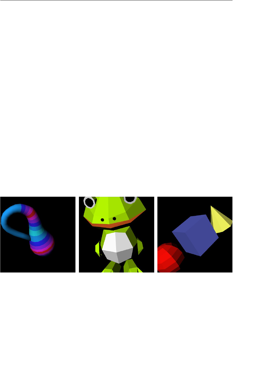
ptg11539634

CHAPTER 10 Advanced Techniques

430

The program traverses the OBJObject objects and its Face objects in the order shown in

Figure 10.28 and stores the information in the arrays

vertices , colors , and indices .

The for statement at line 465 loops, extracting each OBJObject one by one from the result

of the earlier parsing. The

for statement at line 467 does the same for each Face object

that makes up the

OBJObject and performs the following steps for each Face :

1. Lines 469 finds the color of the Face using materialName and stores the color in

color . Line 468 stores the normal of the face in faceNomal for later use.

2. The for statement at line 471 loops, extracting vertex indices from the face, storing

its vertex position in

vertices (lines 477 to 479), and storing the r, g, and b compo-

nents of the color in

colors (lines 482 to 484). The code from line 486 handles

normals. OBJ files may or may not contain normals, so line 487 checks for that. If

normals are found in the OBJ file, lines 487 to 489 store them in

normals . Lines 492

to 494 then store the normals this program generates.

Once you complete these steps for all

OBJObjects , you are ready to draw. Line 502 returns

the information for drawing the model in a

DrawingInfo object, which manages the

vertex information that has to be written in the buffer object, as described previously.

Although this has been, by necessity, a rapid explanation, at this stage you should under-

stand how the contents of the OBJ file can be read in, parsed, and displayed with WebGL.

If you want to read multiple model files in a single scene, you would repeat the preceding

processes. There are several other models stored as OBJ files in the

resources directory of

the sample programs, which you can look at and experiment with to confirm your under-

standing (see Figure 10.29 ).

Figure 10.29 Various 3D models

Handling Lost Context

WebGL uses the underlying graphics hardware, which is a shared resource managed by the

operating system. There are several situations where this resource can be “taken away,”

resulting in information stored within the graphics hardware being lost. These include

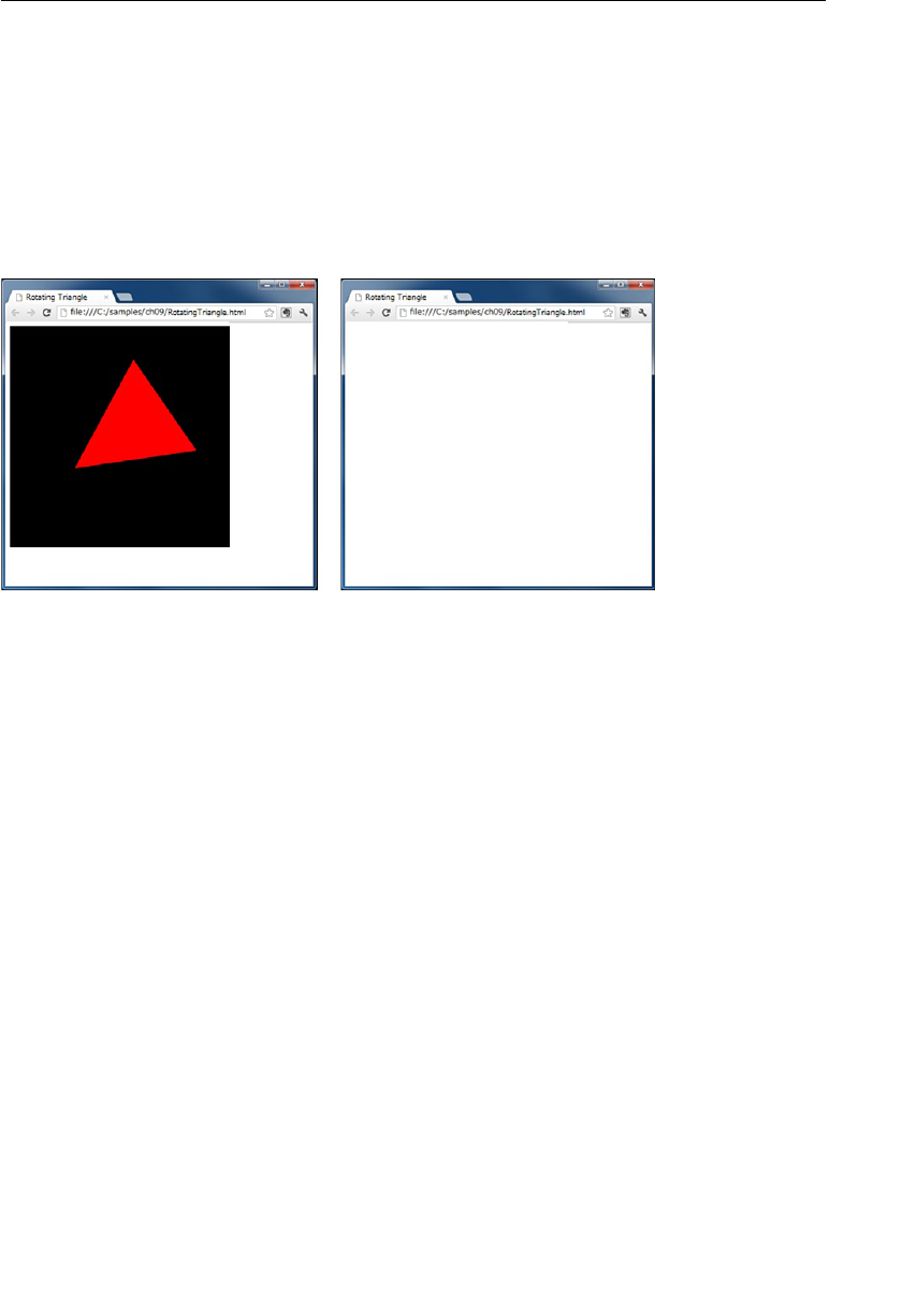
ptg11539634

Handling Lost Context 431

situations when another program takes over the hardware or when the machine hiber-

nates. When this happens, information that WebGL uses to draw correctly, its “context,”

can be lost. A good example is when you run a WebGL program on a notebook PC or

smart phone and it enters hibernation mode. Often, an error message is displayed before

the machine hibernates. When the machine awakes after you press the power button,

the system returns to the original state, but browser that is running the WebGL program

may display nothing on the screen, as on the right side of Figure 10.30 . Because the back-

ground color of the web page that this sample program draws is white, the web browser

shows a completely white screen.

Before Hibernation After Hibernation

Figure 10.30 WebGL program stops after returning from a hibernation mode

For example, if you are running

RotatingTriangle , the following message may be

displayed on the console:

WebGL error CONTEXT_LOST_WEBGL in uniformMatrix4fv([object WebGLUniformLocation,

false, [object Float32Array]]

This indicates that the error occurred when the program performed the gl.uniformMa-

trix4fv() either before the system entered the hibernation mode or on return from hiber-

nation. The error message will differ slightly depending on what the program was trying

to do at the time of hibernation. In this section, we will explain how to deal with this

problem.

How to Implement Handling Lost Context

As previously discussed, context can be lost for any number of reasons. However, WebGL

supports two events to indicate state changes within the system: a context lost event

(

webglcontextlost ) and a context restore event ( webglcontextrestored ). See Table 10.4 .

ptg11539634

CHAPTER 10 Advanced Techniques

432

Table 10.4 The Context Events

Event Description

Webglcontextlost Occurs when the rendering context for WebGL is lost

webglcontextrestored Occurs when the browser completes a reset of the WebGL system

When the context lost event occurs, the rendering context acquired by

getWebGLContext()

(that is

gl in the sample programs) becomes invalid, and any operations carried out using

the

gl context are invalidated. These processes include creating buffer objects and texture

objects, initializing shaders, setting the clear color, and more. After the browser resets the

WebGL system, the context restore event is generated, and your program needs to redo

these operations. The other variables in your JavaScript program are not affected and can

be used as normal.

Before taking a look at the sample program, you need to use the

addEventListener()

method of the

<canvas> to register the event handlers for the context lost event and the

context restore event. This is because the

<canvas> does not support a specific property

that you can use to register context event handlers. Remember that in previous examples

you used the

onmousedown property of <canvas> to register the event handler for the

mouse event.

canvas.addEventListener(type, handler, useCapture)

<canvas> element.

Parameters type Specifies the name of the event to listen for (string).

handler Specifies the event handler to be called when the event

occurs. This function is called with one argument (event

object).

useCapture Specifies whether the event needs to be captured or not

(boolean). If

true , the event is not dispatched to other

elements. If

false , the event is dispatched to others.

Return value None

Sample Program (RotatingTriangle_contextLost.js)

In this section, you will construct a sample program, RotatingTriangle_contextLost ,

which modifies

RotatingTriangle to make it possible to deal with the context lost event

(shown in Figure 10.30 ). The sample program is shown in Listing 10.23 .

ptg11539634

Handling Lost Context 433

Listing 10.23 RotatingTriangle_contextLost.js

1 // RotatingTriangle_contextLost.js

…

16 function main() {

17 // Retrieve <canvas> element

18 var canvas = document.getElementById(‘webgl’);

20 // Register event handler for context lost and restored events

21 canvas.addEventListener(‘webglcontextlost’, contextLost, false);

22 canvas.addEventListener(‘webglcontextrestored’, function(ev)

➥{ start(canvas); }, false);

24 start(canvas); // Perform WebGL-related processes

25 }

…

29 // Current rotation angle

30 var g_currentAngle = 0.0; // Changed from local variable to global

31 var g_requestID; // The return value of requestAnimationFrame()

33 function start(canvas) {

34 // Get the rendering context for WebGL

35 var gl = getWebGLContext(canvas);

…

41 // Initialize shaders

42 if (!initShaders(gl, VSHADER_SOURCE, FSHADER_SOURCE)) {

…

45 }

47 var n = initVertexBuffers(gl); // Set vertex coordinates

…

55 // Get storage location of u_ModelMatrix

56 var u_ModelMatrix = gl.getUniformLocation(gl.program, ‘u_ModelMatrix’);

…

62 var modelMatrix = new Matrix4(); // Create a model matrix

64 var tick = function() { // Start drawing

65 g_currentAngle = animate(g_currentAngle); // Update rotation angle

66 draw(gl, n, g_currentAngle, modelMatrix, u_ModelMatrix);

67 g_requestID = requestAnimationFrame(tick, canvas);

68 };

69 tick();

70 }

72 function contextLost(ev) {

// Event handler for context lost event

ptg11539634

CHAPTER 10 Advanced Techniques

434

73 cancelAnimationFrame(g_requestID); // Stop animation

74 ev.preventDefault(); // Prevent the default behavior

75 }

The processing of the context lost event has no implications for the shaders, so let’s focus

on the

main() function in the JavaScript program starting at line 16. Line 21 registers the

event handler for the context lost event, and line 22 registers the event handler for the

context restore event. The

main() function ends by calling the function start() at

line 24.

The

start() function, defined at line 33, contains the same steps as in RotatingTriangle.

js . They are the processes you have to redo when the context lost event occurs. There are

two changes from

RotatingTriangle.js to handle lost context.

First, the current rotation angle, at line 65, is stored in a global variable

g_currentAngle

(line 30) instead of a local variable. This allows you to draw the triangle using the angle

held in the global variable when a context restore event occurs. Line 67 stores the return

value of

requestAnimationFrame() in the global variable g_requestID (line 31). This is

used to cancel the registration of the function when the context lost event occurs.

Let’s take a look at the actual event handlers. The event handler for the context lost event,

contextLost() , is defined at line 72 and has only two lines. Line 73 cancels the regis-

tration of the function used to carry out the animation, ensuring no further attempt at

drawing is made until the context is correctly restored. Then at Line 74 you prevent the

browser’s default behavior for this event. This is because, by default, the browser doesn’t

generate the context restore event. However, in our case, the event is needed, so you must

prevent this default behavior.

The event handler for the context restore event is straightforward and makes a call to

start() , which rebuilds the WebGL context. This is carried out by registering the event

handler at line 22, which calls

start() by using an anonymous function.

Note that when a context lost event occurs, the following alert is always displayed on the

console:

WARNING: WebGL content on the page might have caused the graphics card to reset

By implementing these handlers for the lost context events, your WebGL applications will

be able to deal with situations where the WebGL context is lost.

Summary

This chapter explained a number of miscellaneous techniques that are useful to know

when creating WebGL applications. Due to space limitations, the explanations have been

kept brief but contain sufficient information for you to master and use the techniques

in your own WebGL applications. Although there are many more techniques you could

learn, we have chosen these because they will help you begin to apply the lessons in this

book to building your own 3D applications.

ptg11539634

Summary 435

As you have seen, WebGL is a powerful tool for creating 3D applications and one that is

capable of creating sophisticated and visually stunning 3D graphics. Our aim in this book

has been to provide you with a step-by-step introduction to the basics of WebGL and give

you a strong enough foundation on which to begin building your own WebGL applica-

tions and exploring further. There are many other resources available to help you in that

exploration. However, our hope is that as you begin to venture out and explore WebGL

yourself, you will return to this book and find it valuable as a reference and guide as you

build your knowledge.

ptg11539634

This page intentionally left blank

ptg11539634

Appendix A

No Need to Swap Buffers in WebGL

For those of you with some experience in developing OpenGL applications on PCs, you may have

noticed that none of the examples in this book seem to swap color buffers, which is something

that most OpenGL implementations require.

As you know, OpenGL uses two buffers: a “front” color buffer and a “back” color buffer with the

contents of the front color buffer being displayed on the screen. Usually, when you draw some-

thing using OpenGL, it is drawn into the back color buffer. When you want to actually display

something, you need to copy the contents of the back buffer to the front buffer to cause it to be

displayed. If you were to draw directly into the front buffer, you would see visual artifacts (such

as flickers) because the screen was being updated before you had finalized the data in the buffer.

To support this dual-buffer approach, OpenGL provides a mechanism to swap the back buffer

and the front buffer. In some systems this is automatic; in others, explicit calls to swap buffers,

such as

glutSwapBuffers() or eglSwapBuffers() , are needed after drawing into the back buffer.

For example, a typical OpenGL application has the following user-defined “display” function:

void display(void) {

// Clear color buffer and depth buffer

glClear(GL_COLOR_BUFFER_BIT | GL_DEPTH_BUFFER_BIT);

draw(); // Draw something

glutSwapBuffers(); // Swap color buffers

}

In contrast, WebGL relies on the browser to automatically manage the display update, reliev-

ing you of the need to do it explicitly in your applications. Referring to Figure A.1 (which is the

same as Figure 2.10 ), when WebGL applications draw something in the color buffer, the browser

detects the drawing and displays the content on the screen. Therefore, WebGL supports only one

color buffer.

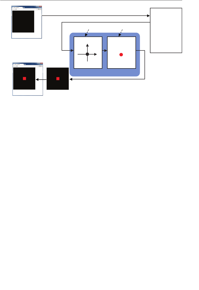
ptg11539634

APPENDIX A No Need to Swap Buffers in WebGL

438

metsyS LGbeW

redahS xetreV tnemgarF

redahS

tpircSavaJ

{ )(niam noitcnuf

…LGbeWteg=lg rav

…

;)…(sredahStini

…

}

noitarepo tnemgarf—rePnoitarepo xetrev—reP

resworB

:noitisoP

)0.1 ,0.0 ,0.0 ,0.0(

0.01 :eziS

:roloC

)0.1 ,0.0 ,0.0 ,0.1(

)daolno( detucexe si margorp tpircSavaJ

reffub roloc eht ot redneR

detucexe era sdohtem detaler—LGbeW

reffuB roloC

yalpsiD

Figure A.1 The processing flow from executing a JavaScript program to displaying the result in

a browser

This approach works, because as seen in the sample programs in this book, all WebGL

programs are executed in the browser by executing the JavaScript in the form of a method

invocation from the browser.

Because the programs are not independently executed, the browser has a chance to

check whether the content of the color buffer was modified after the JavaScript program

executes and exits. If the contents have been modified, the browser is responsible for

ensuring it is displayed on the screen.

For example, in

HelloPoint1 , we execute the JavaScript function ( main() ) from the HTML

file (

HelloPoint1.html ) as follows:

This causes the browser to execute the JavaScript function main() after loading the <body>

element. Within

main() , the draw operation modifies the color buffer.

main(){

…

// Draw a point

gl.drawArrays(gl.POINTS, 0, 1);

}

When main() exits, the control returns to the browser that called the function. The

browser then checks the content of the color buffer, and if anything has been changed,

causes it to be displayed. One useful side effect of this approach is that the browser

ptg11539634

No Need to Swap Buffers in WebGL 439

handles combining the color buffer with the rest of the web page, allowing you to

combine 3D graphics with your web pages. Note that

HelloPoint1 shows only the

<canvas> element on the page, because HelloPoint1.html contains no other elements

than the

<canvas> element.

This implies that if you call methods that return control to the browser, such as alert()

confirm() , the browser may then display the contents of the color buffer to the screen.

This may not be what you expect, so take care when using these methods in your WebGL

programs.

The browser behaves in the same way when JavaScript draws something in an event

handler. This is because the event handler is also called from the browser, and then the

control is returned to the browser after the handler exits.

ptg11539634

This page intentionally left blank

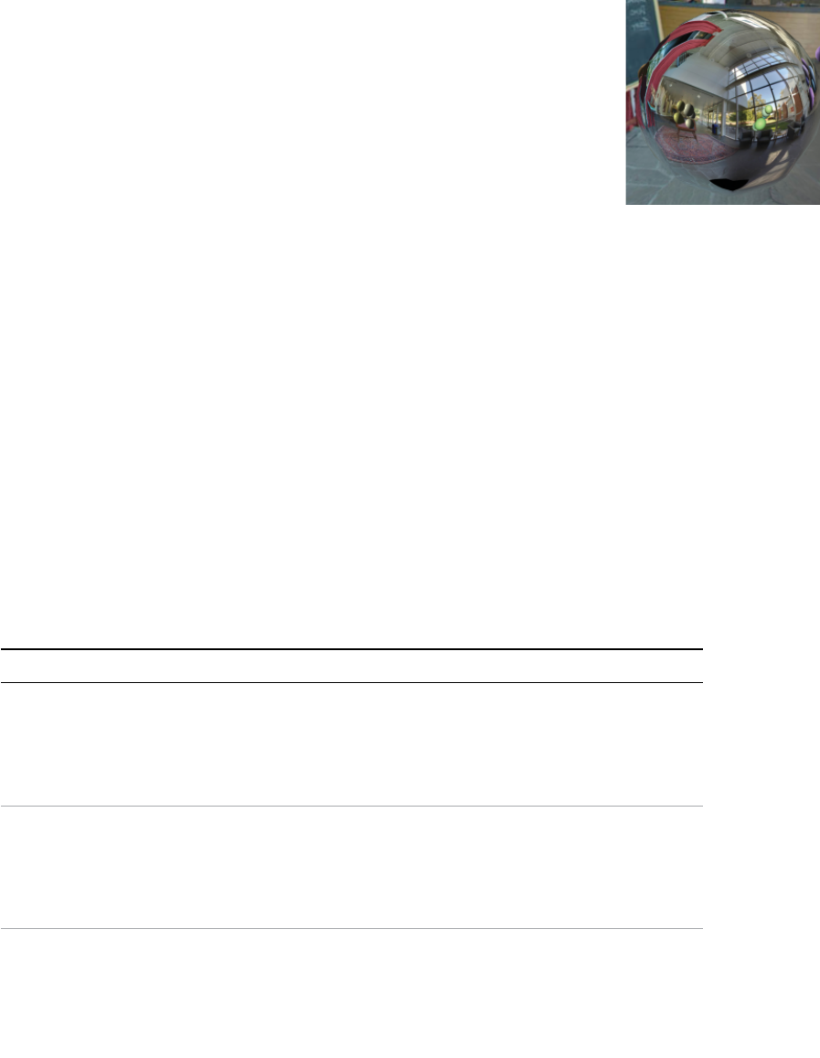
ptg11539634

Appendix B

Built-In Functions of GLSL ES 1.0

This appendix details all embedded functions supported by GLSL ES 1.0, including

many that are not explained in this book but which are often used in programming

shaders.

Note that, in all but texture lookup functions, the operations on vector or matrix argu-

ments are carried out component-wise. For example,

vec2 deg = vec2(60, 80);

vec2 rad = radians(deg);

In these examples, the components of the variable rad are assigned values converted

from 60 and 80 degrees, respectively.

Angle and Trigonometry Functions

Syntax Description

float radians(float degree )

vec2 radians(vec2 degree )

vec3 radians(vec3 degree )

vec4 radians(vec4 degree )

Converts degrees to radians; that is, π * degree /180.

float degrees(float radian )

vec2 degrees(vec2 radian )

vec3 degrees(vec3 radian )

vec4 degrees(vec4 radian )

Converts radians to degrees; that is, 180 * radian /π.

ptg11539634

APPENDIX B Built-In Functions of GLSL ES 1.0

442

Syntax Description

float sin(float angle )

vec2 sin(vec2 angle )

vec3 sin(vec3 angle )

vec4 sin(vec4 angle )

The standard trigonometric sine function. angle is in

radians.

The range of the return value is [–1, 1].

float cos(float angle )

vec2 cos(vec2 angle )

vec3 cos(vec3 angle )

vec4 cos(vec4 angle )

The standard trigonometric cosine function. angle is in

radians.

The range of the return value is [–1, 1].

float tan(float angle )

vec2 tan(vec2 angle )

vec3 tan(vec3 angle )

vec4 tan(vec4 angle )

The standard trigonometric tangent function. angle is in

radians.

float asin(float x )

vec2 asin(vec2 x )

vec3 asin(vec3 x )

vec4 asin(vec4 x )

Arc sine. Returns an angle (in radians) whose sine is

x . The range of the return value is [–π/2, π/2]. Results

are undefined if x > –1 or x > +1.

float acos(float x )

vec2 acos(vec2 x )

vec3 acos(vec3 x )

vec4 acos(vec4 x )

Arc cosine. Returns an angle (in radians) whose cosine

is x . The range of the return value is [0, π]. Results are

undefined if x > –1 or x > +1.

float atan(float y, float x )

vec2 atan(vec2 y, vec2 x )

vec3 atan(vec3 y, vec3 x )

vec4 atan(vec4 y, vec4 x )

Arc tangent. Returns an angle (in radians) whose

tangent is y / x . The signs of x and y are used to deter-

mine what quadrant the angle is in. The range of the

return value is [–π, π]. Results are undefined if x and y

are both 0.

Note, for vectors, this is a component-wise operation.

float atan(float y_over_ x )

vec2 atan(vec2 y_over_ x )

vec3 atan(vec3 y_over_ x )

vec4 atan(vec4 y_over_ x )

Arc tangent. Returns an angle whose tangent is y_

over_x . The range of the return value is [–π/2, π/2].

Note, for vectors, this is a component-wise operation.

ptg11539634

Exponential Functions 443

Exponential Functions

Syntax Description

float pow(float x, float y )

vec2 pow(vec2 x, vec2 y )

vec3 pow(vec3 x, vec3 y )

vec4 pow(vec4 x, vec4 y )

Returns x raised to the y power; that is, x

y .

Results are undefined if x < 0.

Results are undefined if x = 0 and y ≤ 0.

Note, for vectors, this is a component-wise operation.

float exp(float x )

vec2 exp(vec2 x )

vec3 exp(vec3 x )

vec4 exp(vec4 x )

Returns the natural exponentiation of x ; that is, e

x .

float log(float x )

vec2 log(vec2 x )

vec3 log(vec3 x )

vec4 log(vec4 x )

Returns the natural logarithm of x ; that is, returns the value

y , which satisfies the equation x = e

y . Results are undefined

if x ≤ 0.

float exp2(float x )

vec2 exp2(vec2 x )

vec3 exp2(vec3 x )

vec4 exp2(vec4 x )

Returns 2 raised to the x power; that is, 2

x .

float log2(float x )

vec2 log2(vec2 x )

vec3 log2(vec3 x )

vec4 log2(vec4 x )

Returns the base 2 logarithm of x ; that is, returns the value

y , which satisfies the equation x =2

y .

Results are undefined if x ≤ 0.

float sqrt(float x )

vec2 sqrt(vec2 x )

vec3 sqrt(vec3 x )

vec4 sqrt(vec4 x )

Returns x.

Results are undefined if x < 0.

float inversesqrt(float x )

vec2 inversesqrt(vec2 x )

vec3 inversesqrt(vec3 x )

vec4 inversesqrt(vec4 x )

Returns 1/ x

Results are undefined if x ≤ 0.

ptg11539634

APPENDIX B Built-In Functions of GLSL ES 1.0

444

Common Functions

Syntax Description

float abs(float x )

vec2 abs(vec2 x )

vec3 abs(vec3 x )

vec4 abs(vec4 x )

Returns the non-negative value of x without

regard to its sign; that is, x if x ≥ 0, otherwise it

returns – x .

float sign(float x )

vec2 sign(vec2 x )

vec3 sign(vec3 x )

vec4 sign(vec4 x )

Returns 1.0 if x > 0, 0.0 if x = 0, or –1.0 if

x < 0.

float floor(float x )

vec2 floor(vec2 x )

vec3 floor(vec3 x )

vec4 floor(vec4 x )

Returns a value equal to the nearest integer that

is less than or equal to x.

float ceil(float x )

vec2 ceil(vec2 x )

vec3 ceil(vec3 x )

vec4 ceil(vec4 x )

Returns a value equal to the nearest integer that

is greater than or equal to x .

float fract(float x )

vec2 fract(vec2 x )

vec3 fract(vec3 x )

vec4 fract(vec4 x )

Returns the fractional part of x ; that is,

x – floor ( x ).

float mod(float x, float y )

vec2 mod(vec2 x, vec2 y )

vec3 mod(vec3 x, vec3 y )

vec4 mod(vec4 x, vec4 y )

vec2 mod(vec2 x, float y )

vec3 mod(vec3 x, float y )

vec4 mod(vec4 x, float y )

Modulus (modulo). Returns the remainder of the

division of x by y; that is, ( x – y * floor ( x / y )).

Given two positive numbers x and y, mod(x, y) is

the remainder of the division of x by y.

Note, for vectors, this is a component-wise

operation.

ptg11539634

Common Functions 445

Syntax Description

float min(float x, float y )

vec2 min(vec2 x, vec2 y )

vec3 min(vec3 x, vec3 y )

vec4 min(vec4 x, vec4 y )

vec2 min(vec2 x, float y )

vec3 min(vec3 x, float y )

vec4 min(vec4 x, float y )

Returns the smallest value; that is, y if y < x ,

otherwise it returns x .

Note, for vectors, this is a component-wise

operation.

float max(float x, float y )

vec2 max(vec2 x, vec2 y )

vec3 max(vec3 x, vec3 y )

vec4 max(vec4 x, vec4 y )

vec2 max(vec2 x, float y )

vec3 max(vec3 x, float y )

vec4 max(vec4 x, float y )

Returns the largest value; that is, y if x < y ,

otherwise it returns x .

Note, for vectors, this is a component-wise

operation.

float clamp(float x, float minVal ,

float maxVal )

vec2 clamp(vec2 x, vec2 minVal ,

vec2 maxVal )

vec3 clamp(vec3 x, vec3 minVal ,

vec3 maxVal )

vec4 clamp(vec4 x, vec4 minVal ,

vec4 maxVal )

vec2 clamp(vec2 x, float minVal ,

float maxVal )

vec3 clamp(vec3 x, float minVal ,

float maxVal )

vec4 clamp(vec4 x, float minVal ,

float maxVal )

Constrains x to lie between minVal and maxVal;

that is, returns min (max ( x , minVal ), maxVal ).

Results are undefined if minVal > maxVal .

ptg11539634

APPENDIX B Built-In Functions of GLSL ES 1.0

446

Syntax Description

float mix(float x, float y, float a )

vec2 mix(vec2 x, vec2 y, float a )

vec3 mix(vec3 x, vec3 y, float a )

vec4 mix(vec4 x, vec4 y, float a )

vec2 mix(vec2 x, float y, vec2 a )

vec3 mix(vec3 x, float y, vec3 a )

vec4 mix(vec4 x, float y, vec4 a )

vec2 mix(vec2 x, vec2 y, vec2 a )

vec3 mix(vec3 x, vec3 y, vec3 a )

vec4 mix(vec4 x, vec4 y, vec4 a )

Returns the linear blend of x and y ; that is, x *

(1– a ) + y * a.

float step(float edge , float x )

vec2 step(vec2 edge , vec2 x )

vec3 step(vec3 edge , vec3 x )

vec4 step(vec4 edge , vec4 x )

vec2 step(float edge , vec2 x )

vec3 step(float edge , vec3 x )

vec4 step(float edge , vec4 x )

Generates a step function by comparing two

values; that is, returns 0.0 if x < edge , otherwise

it returns 1.0.

float smoothstep(float edge0 ,

float edge1 , float x )

vec2 smoothstep(vec2 edge0 ,

vec2 edge1 , vec2 x )

vec3 smoothstep(vec3 edge0 ,

vec3 edge1 , vec3 x )

vec4 smoothstep(vec4 edge0 ,

vec4 edge1 , vec4 x )

Hermite interpolation.

Returns 0.0 if x ≤ edge0 and 1.0 if x ≥ edge1

and performs smooth Hermite interpolation

between 0 and 1 when edge0 < x < edge1 . This

is equivalent to:

// genType is float, vec2, vec3, or vec4

genType t;

t = clamp (( x – edge0 ) / ( edge1 – edge0 ), 0, 1);

return t * t * (3 – 2 * t);

Results are undefined if edge0 ≥ edge1 .

The following functions determine which components of their arguments will be used

depending on the functionality of the function.

ptg11539634

Geometric Functions 447

Geometric Functions

Syntax Description

float length(float x )

float length(vec2 x )

float length(vec3 x )

float length(vec4 x )

Returns the length of vector x .

float distance(float p0 , float p1 )

float distance(vec2 p0 , vec2 p1 )

float distance(vec3 p0 , vec3 p1 )

float distance(vec4 p0 , vec4 p1 )

Returns the distance between p0 and p1 ; that is,

length ( p0 – p1 ).

float dot(float x , float y )

float dot(vec2 x , vec2 y )

float dot(vec3 x , vec3 y )

float dot(vec4 x , vec4 y )

Returns the dot product of x and y , in case of

vec3, x [0]* y [0]+ x [1]* y [1]+ x [2]* y [2].

vec3 cross(vec3 x , vec3 y ) Returns the cross product of x and y , in case of

vec3,

result[0] = x [1]* y [2] — y [1]* x [2]

result[1] = x [2]* y [0] — y [2]* x [0]

result[2] = x [0]* y [1] — y [0]* x [1]

float normalize(float x )

vec2 normalize(vec2 x )

vec3 normalize(vec3 x )

vec4 normalize(vec4 x )

Returns a vector in the same direction as x but

with a length of 1; that is, x /length( x ).

float faceforward(float N , float I ,

float Nref )

vec2 faceforward(vec2 N , vec2 I ,

vec2 Nref )

vec3 faceforward(vec3 N , vec3 I ,

vec3 Nref )

vec4 faceforward(vec4 N , vec4 I ,

vec4 Nref )

Reverse the normal. Adjust the vector N according to

the incident vector I and the reference vector Nref .

If dot( Nref , I ) < 0 return N , otherwise return – N .

ptg11539634

APPENDIX B Built-In Functions of GLSL ES 1.0

448

Syntax Description

float reflect(float I , float N )

vec2 reflect(vec2 I , vec2 N )

vec3 reflect(vec3 I , vec3 N )

vec4 reflect(vec4 I , vec4 N )

Calculate reflection vector. For the incident vector

I and surface orientation N , returns the reflection

direction: I – 2 * dot( N , I ) * N

N must already be normalized to achieve the

desired result.

float refract(float I , float N ,

float eta )

vec2 refract(vec2 I , vec2 N , float

eta

)

vec3 refract(vec3 I , vec3 N , float

eta

)

vec4 refract(vec4 I , vec4 N , float

eta

)

Calculate the change in direction of light due to its

medium by calculating the incident vector using the

ratio of indices of refraction. For the incident vector

I and surface normal N , and the ratio of indices of

refraction eta , return the refraction vector using the

following:

k = 1.0 – eta * eta * (1.0 – dot( N , I ) * dot( N , I ))

if (k < 0.0)

// genTyp is float, vec2, vec3, or vec4

return genType(0.0)

else

return eta * I — ( eta * dot( N , I ) + sqrt(k)) * N

The input parameters for the incident vector I and

the surface normal N must already be normalized.

Matrix Functions

Syntax Description

mat2 matrixCompMult(mat2 x , mat2 y )

mat3 matrixCompMult(mat3 x , mat3 y )

mat4 matrixCompMult(mat4 x , mat4 y )

Multiply matrix x by matrix y component-wise; that

is, if result = matrixCompMatrix( x , y ) then

result[i][j] = x [i][j] * y [i][j].

ptg11539634

Vector Functions 449

Vector Functions

Syntax Description

bvec2 lessThan(vec2 x, vec2 y )

bvec3 lessThan(vec3 x, vec3 y )

bvec4 lessThan(vec4 x, vec4 y )

bvec2 lessThan(ivec2 x, ivec2 y )

bvec3 lessThan(ivec3 x, ivec3 y )

bvec4 lessThan(ivec4 x, ivec4 y )

Return the component-wise comparison of

x < y .

bvec2 lessThanEqual(vec2 x, vec2 y )

bvec3 lessThanEqual(vec3 x, vec3 y )

bvec4 lessThanEqual(vec4 x, vec4 y )

bvec2 lessThanEqual(ivec2 x, ivec2 y )

bvec3 lessThanEqual(ivec3 x, ivec3 y )

bvec4 lessThanEqual(ivec4 x, ivec4 y )

Return the component-wise comparison of

x ≤ y .

bvec2 greaterThan(vec2 x , vec2 y )

bvec3 greaterThan(vec3 x , vec3 y )

bvec4 greaterThan(vec4 x , vec4 y )

bvec2 greaterThan(ivec2 x , ivec2 y )

bvec3 greaterThan(ivec3 x , ivec3 y )

bvec4 greaterThan(ivec4 x , ivec4 y )

Return the component-wise comparison of

x > y .

bvec2 greaterThanEqual(vec2 x , vec2 y )

bvec3 greaterThanEqual(vec3 x , vec3 y )

bvec4 greaterThanEqual(vec4 x , vec4 y )

bvec2 greaterThanEqual(ivec2 x , ivec2 y )

bvec3 greaterThanEqual(ivec3 x , ivec3 y )

bvec4 greaterThanEqual(ivec4 x , ivec4 y )

Return the component-wise comparison of

x ≥ y .

ptg11539634

APPENDIX B Built-In Functions of GLSL ES 1.0

450

Syntax Description

bvec2 equal(vec2 x , vec2 y )

bvec3 equal(vec3 x , vec3 y )

bvec4 equal(vec4 x , vec4 y )

bvec2 equal(ivec2 x , ivec2 y )

bvec3 equal(ivec3 x , ivec3 y )

bvec4 equal(ivec4 x , ivec4 y )

Return the component-wise comparison of

x == y .

bvec2 notEqual(vec2 x , vec2 y )

bvec3 notEqual(vec3 x , vec3 y )

bvec4 notEqual(vec4 x , vec4 y )

bvec2 notEqual(ivec2 x , ivec2 y )

bvec3 notEqual(ivec3 x , ivec3 y )

bvec4 notEqual(ivec4 x , ivec4 y )

Return the component-wise comparison of

x != y .

bool any(bvec2 x )

bool any(bvec3 x )

bool any(bvec4 x )

Return

true if any component of x is true .

bool all(bvec2 x )

bool all(bvec3 x )

bool all(bvec4 x )

Return

true only if all components of x are

true .

bvec2 not(bvec2 x )

bvec3 not(bvec3 x )

bvec4 not(bvec4 x )

Return the component-wise logical comple-

ment of x .

ptg11539634

Texture Lookup Functions 451

Texture Lookup Functions

Syntax Description

vec4 texture2D(

sampler2D sampler , vec2 coord )

vec4 texture2D(

sampler2D sampler , vec2 coord ,

float bias )

vec4 texture2DProj(

sampler2D sampler , vec3 coord )

vec4 texture2DProj(

sampler2D sampler , vec3 coord ,

float bias )

vec4 texture2DProj(

sampler2D sampler , vec4 coord )

vec4 texture2DProj(

sampler2D sampler , vec4 coord ,

float bias )

vec4 texture2DLod(

sampler2D sampler , vec2 coord ,

float lod )

vec4 texture2DProjLod(

sampler2D sampler , vec3 coord ,

float lod )

vec4 texture2DProjLod(

sampler2D sampler , vec4 coord ,

float lod )

Use the texture coordinate coord

to read out texel values in the

2D texture currently bound to

sampler . For the projective (Proj)

versions, the texture coordinate

( coord .s, coord .t) is divided by

the last component of coord .

The third component of coord

is ignored for the vec4 coord

variant. The bias parameter

is only available in fragment

shaders. It specifies the value

to add the current lod when a

MIPMAP texture is bound to

sampler .

vec4 textureCube(

samplerCube sampler , vec3 coord )

vec4 textureCube(

samplerCube sampler , vec3 coord ,

float bias )

vec4 textureCubeLod(

samplerCube sampler , vec3 coord ,

float lod )

Use the texture coordinate

coord to read out a texel from

the cube map texture currently

bound to sampler . The direction

of coord is used to select the

face from the cube map texture.

ptg11539634

This page intentionally left blank

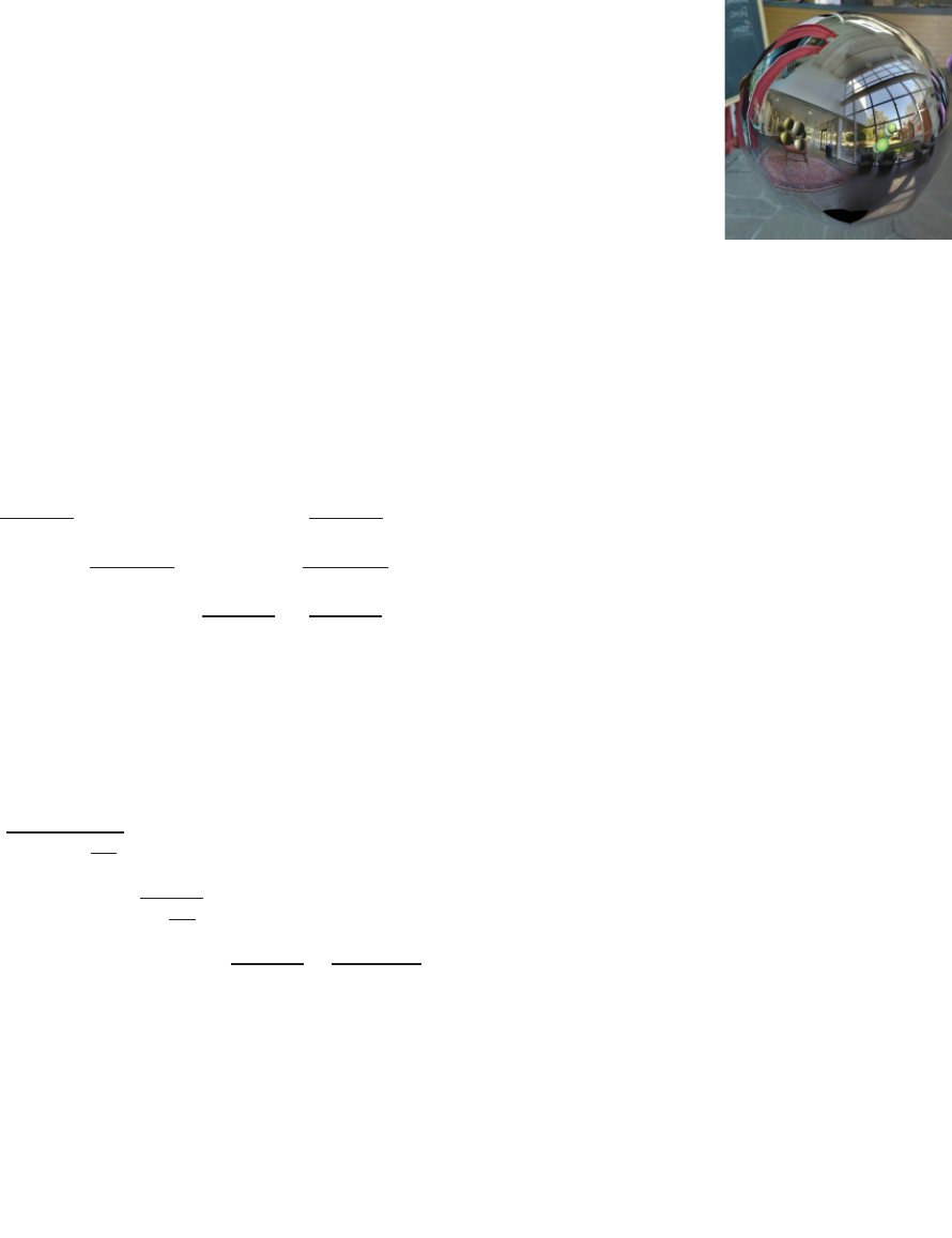
ptg11539634

Appendix C

Projection Matrices

Orthogonal Projection Matrix

The following matrix is created by Matrix4.setOrtho(left , right , bottom , top , near , far) .

200

00 0 1

right left

tfelthgirtfelthgir

top bottom

top bottom top bottom

far near

far near far near

+⎤⎡ −⎥⎢ −− ⎥⎢ +⎥⎢ −⎥⎢ −− ⎥⎢ +⎥⎢ −−

⎥⎢ −−

⎥⎢ ⎥⎢ ⎦⎣

Perspective Projection Matrix

The following matrix is created by Matrix4.setPerspective(fov , aspect , near , far) .

100 0

*tan( )

1000

tan( )

2* *

0010

fov

aspect

fov

far near far near

⎤⎡ ⎥⎢ ⎥⎢ ⎥⎢ ⎥⎢ ⎥⎢ ⎥⎢ ⎥⎢ ⎥⎢ +

−−⎥⎢ −−

⎥⎢ ⎥⎢ −⎦⎣

ptg11539634

This page intentionally left blank

ptg11539634

Appendix D

WebGL/OpenGL: Left or Right Handed?

In Chapter 2 , “Your First Step with WebGL,” the coordinate system of WebGL was

introduced as a right-handed system. However, you will probably come across tuto-

rials and other material on the web that contradict this. In this appendix, you’ll

learn the “real” coordinate systems used by WebGL by examining what will happen

when something is drawn using WebGL’s default settings. Because WebGL is based

on OpenGL, what you learn is equally applicable to OpenGL. You should read this

appendix after reading Chapter 7 , “Toward the 3D World,” because it refers back to

sample programs and explanations in that chapter.

Let’s start by referring to the “font of all knowledge”: the original specification.

Specifically, the authorized specification of OpenGL ES 2.0, which is the base specifi-

cation of WebGL, published by the Khronos group,

1 states in Appendix B :

7. The GL does not force left- or right-handedness on any of its coordinate systems.

If this is the case, and WebGL is agnostic about handedness, then why do many books

and tutorials, and in fact this book, describe WebGL as right handed? Essentially, it’s

a convention. When you are developing your applications, you need to decide which

coordinate system you are using and stick with it. That’s true for your applications,

but it’s also true for the many libraries that have been developed to help people use

WebGL (and OpenGL). Many of those libraries choose to adopt the right-handed

convention, so over time it becomes the accepted convention and then becomes

synonymous with the GL itself, leading people to believe that the GL is right handed.

So why the confusion? If everybody accepts the same convention, there shouldn’t be

a problem. That’s true, but the complication arises because WebGL (and OpenGL) at

certain times requires the GL to choose a handedness to carry out its operations, a

default behavior if you will, and that default isn’t always right handed!

1. www.khronos.org/registry/gles/specs/2.0/es_cm_spec_2.0.24.pdf

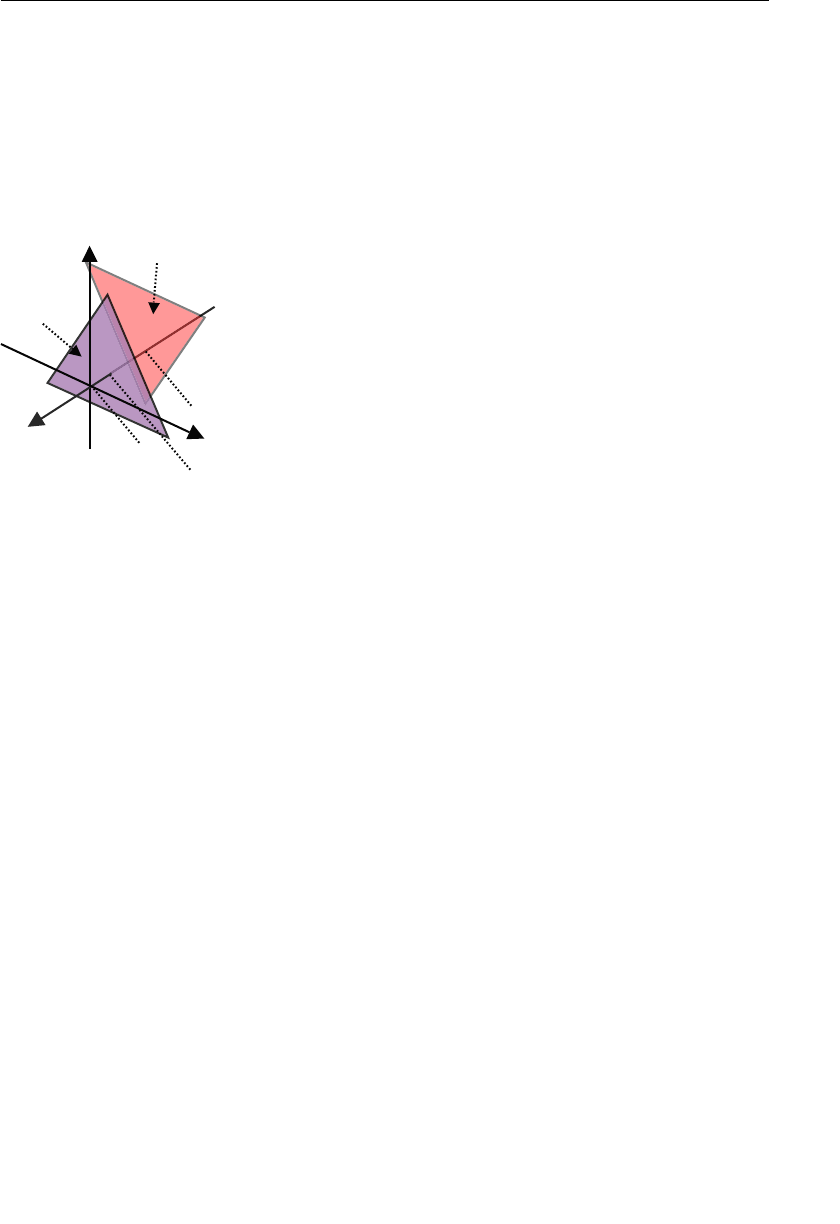
ptg11539634

APPENDIX D WebGL/OpenGL: Left or Right Handed?

456

In this appendix, we explore the default behavior of WebGL to give you a clearer under-

standing of the issue and how to factor this into your own applications.

To begin the exploration of WebGL’s default behavior, let’s construct a sample program

CoordinateSystem as a test bed for experimentation. We’ll use this program to go back to

first principals, starting with the simplest method of drawing triangles and then adding

features to explore how WebGL draws multiple objects. The goal of our sample program is

to draw a blue triangle at –0.1 on the z-axis and then a red triangle at –0.5 on the z-axis.

Figure D.1 shows the triangles, their z coordinates, and colors.

der

eul

5.0—

0.0

1.0—

Figure D.1 The triangles used in this appendix and their colors

As this appendix will show, to achieve our relatively modest goal, we actually have to get

a number of interacting features to work together, including the basic drawing, hidden

surface removal, and viewing volume. Unless all three are set up correctly, you will get

unexpected results when drawing, which can lead to confusion about left and right

handedness.

Sample Program CoordinateSystem.js

Listing D.1 shows CoordinateSystem.js . The code for error processing and some

comments have been removed to allow all lines in the program to be shown in a limited

space, but as you can see, it is a complete program.

Listing D.1 CoordinateSystem

1 // CoordinateSystem.js

2 // Vertex shader program

3 var VSHADER_SOURCE =

4 ‘attribute vec4 a_Position;n’ +

5 ‘attribute vec4 a_Color;n’ +

6 ‘varying vec4 v_Color;n’ +

7 ‘void main() {n’ +

8 ‘ gl_Position = a_Position;n’ +

9 ‘ v_Color = a_Color;n’ +

ptg11539634

Sample Program CoordinateSystem.js 457

10 ‘}n’;

12 // Fragment shader program

13 var FSHADER_SOURCE =

14 ‘#ifdef GL_ESn’ +

15 ‘precision mediump float;n’ +

16 ‘#endifn’ +

17 ‘varying vec4 v_Color;n’ +

18 ‘void main() {n’ +

19 ‘ gl_FragColor = v_Color;n’ +

20 ‘}n’;

22 function main() {

23 var canvas = document.getElementById(‘webgl’); // Retrieve <canvas>

24 var gl = getWebGLContext(canvas); // Get the context for WebGL

25 initShaders(gl, VSHADER_SOURCE, FSHADER_SOURCE);// Initialize shaders

26 var n = initVertexBuffers(gl); // Set vertex coordinates and colors

28 gl.clearColor(0.0, 0.0, 0.0, 1.0); // Specify the clear color

29 gl.clear(gl.COLOR_BUFFER_BIT); // Clear <canvas>

30 gl.drawArrays(gl.TRIANGLES, 0, n); // Draw the triangles

31 }

33 function initVertexBuffers(gl) {

34 var pc = new Float32Array([ // Vertex coordinates and color

35 0.0, 0.5, -0.1, 0.0, 0.0, 1.0, // The blue triangle in front

36 -0.5, -0.5, -0.1, 0.0, 0.0, 1.0,

37 0.5, -0.5, -0.1, 1.0, 1.0, 0.0,

39 0.5, 0.4, -0.5, 1.0, 1.0, 0.0, // The red triangle behind

40 -0.5, 0.4, -0.5, 1.0, 0.0, 0.0,

41 0.0, -0.6, -0.5, 1.0, 0.0, 0.0,

42 ]);

43 var numVertex = 3; var numColor = 3; var n = 6;

45 // Create a buffer object and write data to it

46 var pcbuffer = gl.createBuffer();

47 gl.bindBuffer(gl.ARRAY_BUFFER, pcbuffer);

48 gl.bufferData(gl.ARRAY_BUFFER, pc, gl.STATIC_DRAW);

50 var FSIZE = pc.BYTES_PER_ELEMENT; // The number of byte

51 var STRIDE = numVertex + numColor; // Calculate the stride

53 // Assign the vertex coordinates to attribute variable and enable it

54 var a_Position = gl.getAttribLocation(gl.program, ‘a_Position’);

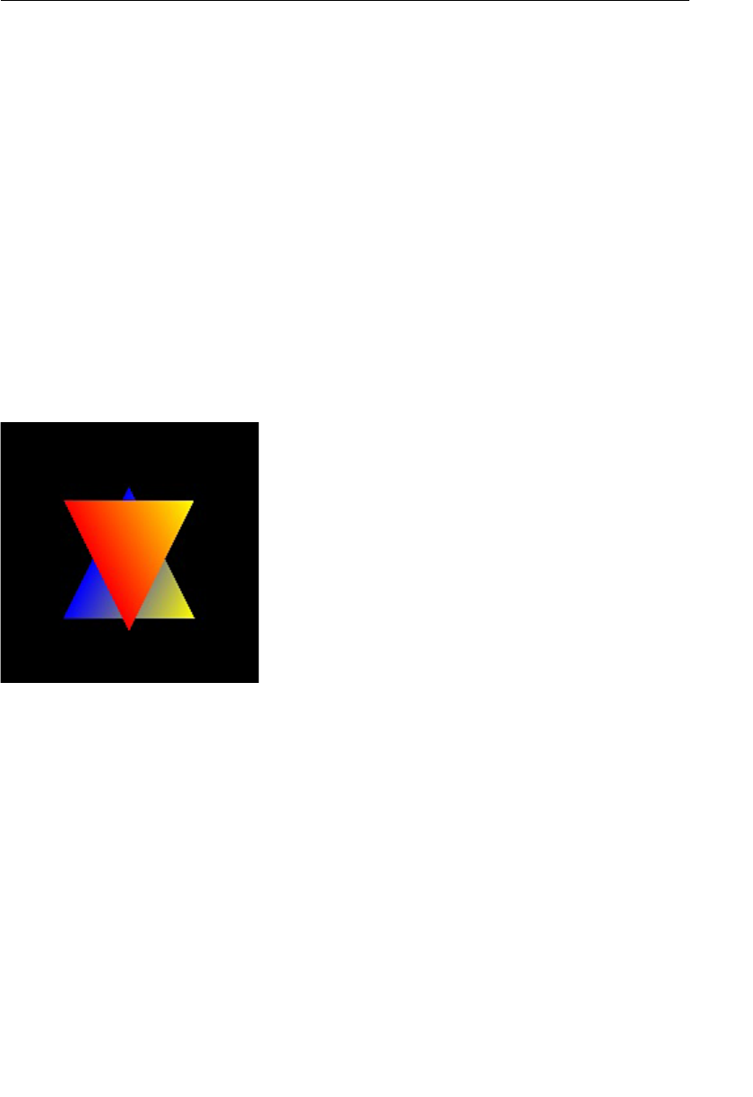
ptg11539634

APPENDIX D WebGL/OpenGL: Left or Right Handed?

458

55 gl.vertexAttribPointer(a_Position, numVertex, gl.FLOAT, false, FSIZE *

➥STRIDE, 0);

56 gl.enableVertexAttribArray(a_Position);

58 // Assign the vertex colors to attribute variable and enable it

59 var a_Color = gl.getAttribLocation(gl.program, ‘a_Color’);

60 gl.vertexAttribPointer(a_Color, numColor, gl.FLOAT, false, FSIZE *

➥STRIDE, FSIZE * numVertex);

61 gl.enableVertexAttribArray(a_Color);

63 return n;

64 }

When the sample program is run, it produces the output shown in Figure D.2 . Although

it’s not easy to see in black and white (remember, you can run these examples in your

browser from the book’s website), the red triangle is in front of the blue triangle. This is

the opposite of what you might expect because lines 32 to 42 specify the vertex coordi-

nates of the blue triangle before the red triangle.

Figure D.2 CoordinateSystem

However, as explained in Chapter 7 , this is actually correct. What is happening is that

WebGL is first drawing the blue triangle, because its vertex coordinates are specified first,

and then it’s drawing the red triangle over the blue triangle. This is a little like oil paint-

ing; once you lay down a layer of paint, anything painted on top has to overwrite the

paint below.

For many newcomers to WebGL, this can be counterintuitive. Because WebGL is a system

for drawing 3D graphics, you’d expect it to “do the right thing” and draw the red triangle

behind the blue one. However, by default WebGL draws in the order specified in the

application code, regardless of the position on the z-axis. If you want WebGL to “do the

right thing,” you are required to enable the Hidden Surface Removal feature discussed in

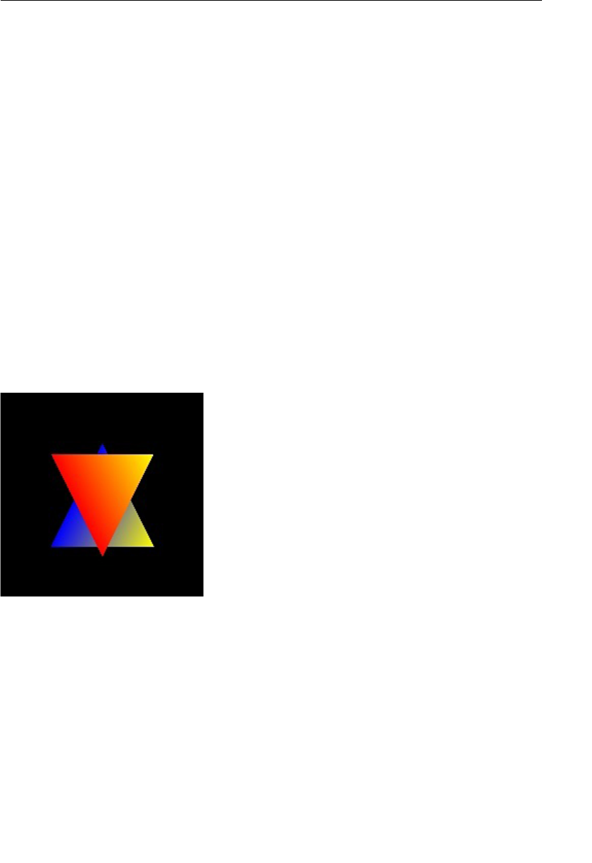
ptg11539634

Hidden Surface Removal and the Clip Coordinate System 459

Chapter 7 . As you saw in Chapter 7 , Hidden Surface Removal tells WebGL to be smart

about the 3D scene and to remove surfaces that are actually hidden. In our case, this

should deal with the red triangle problem because in the 3D scene, most of the red trian-

gle is hidden behind the blue one.

Hidden Surface Removal and the Clip Coordinate

System

Let’s turn on Hidden Surface Removal in our sample program and examine its effect. To

do that, enable the function using

gl.enable(gl.DEPTH_TEST) , clear the depth buffer, and

then draw the triangles. First, you add the following at line 27.

27 gl.enable(gl.DEPTH_TEST);

Then you modify line 29 as follows:

29 gl.clear(gl.COLOR_BUFFER_BIT | gl.DEPTH_BUFFER_BIT);

Now if you rerun the program after making these changes, you’d expect to see the

problem resolved and the blue triangle in front of the red one. However, what you actu-

ally see is that the red triangle is still in front. Again, although it’s difficult to see in black

and white, Figure D.3 shows the result.

Figure D.3 CoordinateSystem using the hidden surface removal function

This is unexpected and is part of the confusion surrounding WebGL’s left versus right

handedness. We have correctly programmed our example based on the belief that WebGL

is right handed, but it seems to be that WebGL is either telling us that –0.5 is located

in front of –0.1 on the z-axis or that WebGL does in fact use the left-handed coordinate

system, where the positive direction of the z-axis points into the screen ( Figure D.4 ).

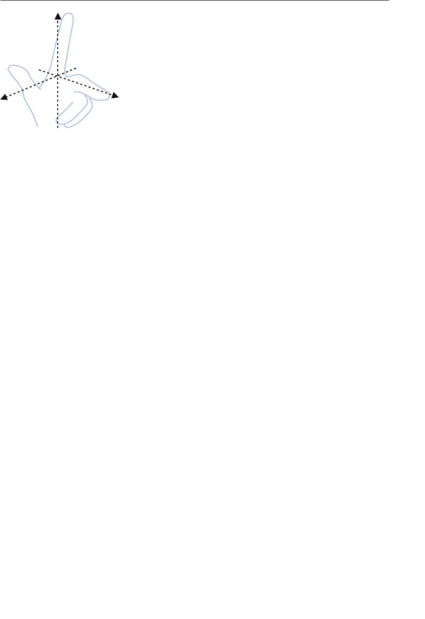
ptg11539634

APPENDIX D WebGL/OpenGL: Left or Right Handed?

460

Figure D.4 The left-handed coordinate system

The Clip Coordinate System and the Viewing Volume

So our application example follows the convention that WebGL is right handed, but

our program clearly shows a left-handed system is in place. What’s the explanation?

Essentially, hidden surface removal, when enabled, uses the clip coordinate system (see

Figure G.5 in Appendix G ), which itself uses the “left-handed” coordinate system, not the

right-handed one.

In WebGL (OpenGL), hidden surface removal is performed using the value of

gl_

Position , the coordinates produced by the vertex shader. As you can see at line 8 in

the vertex shader in Listing D.1 ,

a_Position is directly assigned to gl_Position in

CoordinateSystem.js . This means that the z coordinate of the red triangle is passed as

–0.5 and that of the blue one is passed as –0.1 to the clip coordinate system (the left-

handed coordinate system). As you know, the positive direction of the z-axis in the left-

handed coordinate system points into the screen, so the smaller value of the z coordinate

(–0.5) is located in front of the bigger one (–0.1). Therefore, it is the right behavior for the

WebGL system to display the red triangle in front of the blue one in this situation.

This obviously contradicts the explanation in Chapter 3 (that WebGL uses the right-

handed coordinate system). So how do we achieve our goal of having the red triangle

displayed behind the blue triangle, and what does this tell us about WebGL’s default

behaviors? Until now, the program hasn’t considered the viewing volume that needs to be

set up correctly for Hidden Surface Removal to work with our coordinate system. When

used correctly, the viewing volume requires that the near clipping plane be located in

front of the far clipping plane (that is near < far ). However, the values of near and far are

the distance from the eye point toward the direction of line of sight and can take any

value. Therefore, it is possible to specify a value of far that is actually smaller than that of

near or even use negative values. (The negative values means the distance from the eye

point toward the opposite direction of line of sight.) Obviously, the values set for near and

far depend on whether we are assuming a right- or left-handed coordinate system.

Returning to the sample program, after setting the viewing volume correctly, let’s

carry out the hidden surface removal. Listing D.2 shows only the differences from

CoordinateSystem.js .

ptg11539634

The Clip Coordinate System and the Viewing Volume 461

Listing D.2 CoordinateSystem_viewVolume.js

1 // CoordinateSystem_viewVolume.js

2 // Vertex shader program

3 var VSHADER_SOURCE =

4 ‘attribute vec4 a_Position;n’ +

5 ‘attribute vec4 a_Color;n’ +

6 ‘uniform mat4 u_MvpMatrix;n’ +

7 ‘varying vec4 v_Color;n’ +

8 ‘void main() {n’ +

9 ‘gl_Position = u_MvpMatrix * a_Position;n’ +

10 ‘v_Color = a_Color;n’ +

11 ‘}n’;

…

23 function main() {

…

29 gl.enable(gl.DEPTH_TEST); // Enable hidden surface removal function

30 gl.clearColor(0.0, 0.0, 0.0, 1.0); // Set the clear color

31 // Get the storage location of u_MvpMatrix

32 var u_MvpMatrix = gl.getUniformLocation(gl.program, ‘u_MvpMatrix’);

34 var mvpMatrix = new Matrix4();

35 mvpMatrix.setOrtho(-1, 1, -1, 1, 0, 1); // Set the viewing volume

36 // Pass the view matrix to u_MvpMatrix

37 gl.uniformMatrix4fv(u_MvpMatrix, false, mvpMatrix.elements);

39 gl.clear(gl.COLOR_BUFFER_BIT | gl.DEPTH_BUFFER_BIT);

40 gl.drawArrays(gl.TRIANGLES, 0, n); // Draw the triangle

41 }

Once you run this sample program, you can see the result shown in Figure D.5 , in which

the blue triangle is displayed in front of the red one.

Figure D.5 CoordinateSystem_viewVolume

ptg11539634

APPENDIX D WebGL/OpenGL: Left or Right Handed?

462

The critical change is that the uniform variable ( u_MvpMatrix ) for passing a view matrix

was added to the vertex shader. It was multiplied by

a_Position , and then its result was

assigned to

gl_Position . Although we used the setOrtho() method to specify the viewing

volume,

setPerspective() has the same result.

What Is Correct?

Let’s compare the process of the vertex shader in CoordinateSystem.js with that in

CoordinateSystem_viewVolume.js .

Line 8 in CoordinateSystem.js :

8 ‘ gl_Position = a_Position;n’ +

became line 9 in CoordinateSystem_viewVolume.js :

9 ‘ gl_Position = u_MvpMatrix * a_Position;n’ +

As you can see, in CoordinateSystem_viewVolume.js , which displays the order of triangles

as was intended, the transformation matrix (in this case, a view matrix) is multiplied by

a vertex coordinate. To understand this operation, let’s examine how to rewrite line 8

CoordinateSystem.js into the form <matrix> * <vertex coordinate> just like line 9 in

CoordinateSystem_viewVolume.js .

Line 8 assigns the vertex coordinate ( a_Position ) to gl_Position directly. To ensure that

the matrix multiplication operation has no effect the <matrix> must have the following

elements (that is, the identity matrix):

⎡

⎣

⎢

⎤

⎦

⎥

1000

0100

0010

0001

Therefore, line 8 in

CoordinateSystem.js actually has the same effect as passing the iden-

tity matrix to

u_MvpMatrix in line 9 in CoordinateSystem_viewVolume.js . In essence, this

matrix is controlling the default behavior of WebGL.

To understand this behavior better, let’s clarify what is happening if the projection matrix

is the identity matrix. You can understand this by using the matrix in Appendix C (see

Figure D.6 ) and the identify matrix to find left , right , top , bottom , near , and far.

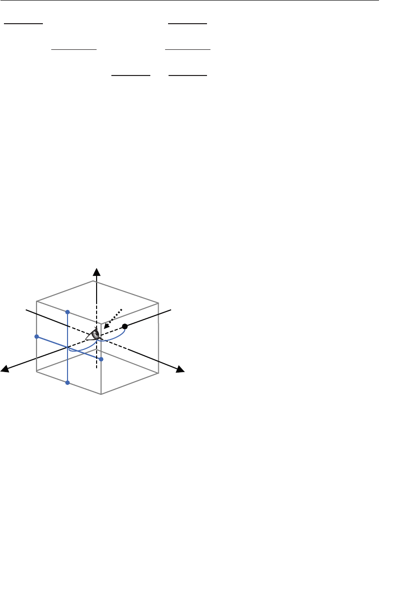
ptg11539634

What Is Correct? 463

200

00 0 1

right left

tfelthgirtfelthgir

top bottom

top bottom top bottom

far near

far near far near

+⎤⎡ −⎥⎢ −− ⎥⎢ +⎥⎢ −⎥⎢ −− ⎥⎢ +⎥⎢ −−

⎥⎢ −−

⎥⎢ ⎥⎢ ⎦⎣

Figure D.6 The projection matrix generated by setOrtho()

In this case, right – left = 2 and right + left = 0, which resolves to left = –1, right = 1. Equally,

far – near =–2 and far + near = 0, resolving to near = 1 and far = –1. That is:

left = -1, right = 1, bottom = -1, top = 1, near = 1, and far = -1

Using these parameters to setOrtho() as follows:

mvpMatrix.setOrtho(-1, 1, -1, 1, 1, -1);

results in near being greater than far . This means that the far clipping plane is placed in

front of the near clipping plane along the direction of the line of sight (see Figure D.7 ).

left=-1.0

top=1.0 Eye point

near=1.0

right=1.0

far=-1.0

bottom= -1.0

Figure D.7 The viewing volume created by the identity matrix

If you specify the viewing volume by yourself, you will observe the same phenomenon

when you specify near > far to

setOrtho() . That is, WebGL (OpenGL) follows the right-

handed coordinate system when you specify the viewing volume in this way.

Then look at the matrix representing the viewing volume in which the objects are

displayed correctly:

mvpMatrix.setOrtho(-1, 1, -1, 1, -1, 1);

ptg11539634

APPENDIX D WebGL/OpenGL: Left or Right Handed?

464

This method generates the following projection matrix:

−

⎡

⎣

⎢

⎤

⎦

⎥

1000

0100

00 10

0001

You will recognize that this matrix is a scaling matrix described in Chapter 4 , “More

Transformations and Basic Animation.” That is the matrix generated by

setScale(1, 1,

-1) . You should note that the scaling factor of the z-axis is –1, meaning that the sign

of the z coordinates will be reversed. So this matrix transforms the conventional right-

handed coordinate system used in this book (and assumed by most WebGL libraries) to

the left-handed coordinate system used in the clip coordinate system by reversing the z

coordinates.

Summary

In summary, we know from the specification that WebGL doesn’t enforce either right

or left handedness. We have seen that many WebGL libraries and applications adopt

the convention that WebGL is right handed, as do we in this book. When WebGL’s

default behavior contradicts this (for example, when working in clip-space where it uses

a left-handed coordinate system), we can compensate programmatically, by reversing,

for example, the z coordinates. This allows us to continue to follow the convention that

WebGL is right handed. However, as previously stated, it’s only a convention. It’s one

that most people follow, but one that will occasionally trip you up if you aren’t aware of

WebGL’s default behaviors and how to handle them.

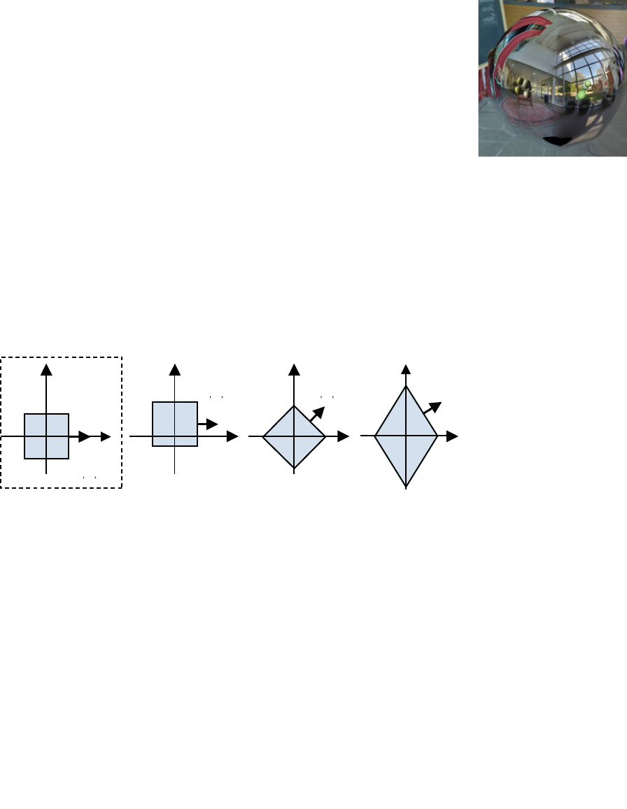
ptg11539634

Appendix E

The Inverse Transpose Matrix

The inverse transpose matrix, previously introduced in Chapter 8 , “Lighting Objects,” is

a matrix that determines the inverse of a given matrix and then transposes it. As shown

in Figure E.1 , the direction of the normal vector of an object is subject to change

depending on the type of the coordinate transformation. However, if you use the

inverse transpose of the model matrix, you can safely ignore this in calculations.

lamroneht

noitcerid

1( 0)0

noitceridlamroneht

1( 0)0

noitceridlamroneht

1( 1)0

noitceridlamroneht

)0,5.0,1(

noitalsnart)1(

)sixa—yehtgnolaetalsnart(

noitator)2(

)seerged54etator(

gnilacs)3(

gnola2ybelacs(

)sixa—yeht

lamronlanigiroeht

Figure E.1 The direction of normal vector changes along with the coordinate transformation

In Chapter 8 , you saw how to use the inverse transpose of the model matrix to trans-

form normals. However, there are actually some cases where you can also determine

the normal vector direction with the model matrix. For instance, when rotating, you

can determine the direction of the normal vector by multiplying the normal vector by

the rotation matrix. When calculating the direction of the normal vector, whether you

resort to the model matrix itself or its inverse transpose depends on which transforma-

tion (translation, rotation, and scaling) is already integrated inside the model matrix.

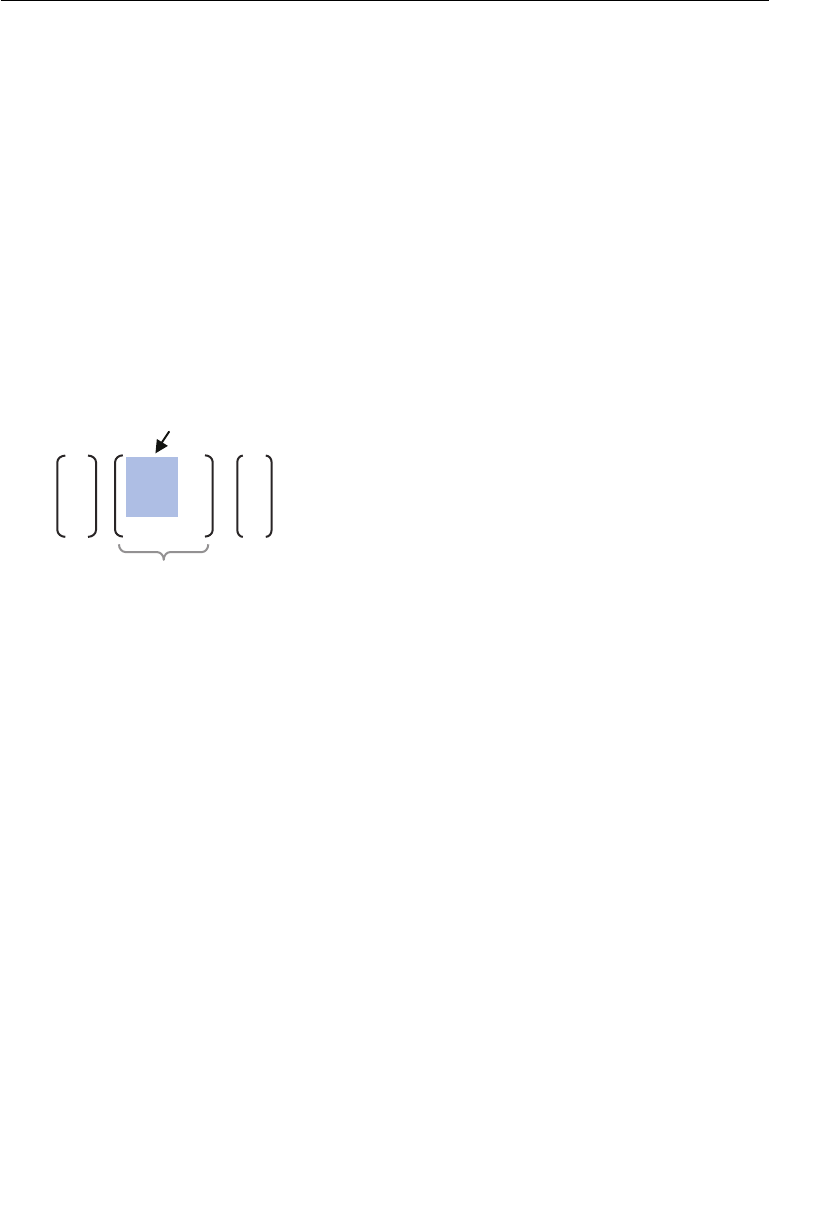
ptg11539634

APPENDIX E The Inverse Transpose Matrix

466

If the model matrix already includes a translation and you multiply the normal by the

model matrix, the normal is translated, resulting in a modification of its orientation. For

example, the normal (1, 0, 0), when translated by 2.0 along the y-axis, is repositioned to

the location (1, 2, 0). You can avoid this problem by using the 3×3 submatrix extracted

from the top left area of the 4×4 model matrix. For example:

attribute vec4 a_Normal; // normal

uniform mat4 u_ModelMatrix; // model matrix

void main() {

…

vec3 normal = normalize(mat3(u_ModelMatrix) * a_Normal.xyz);

…

}

The values located in the rightmost column determine the scale of the displacement

produced by the translation matrix, as illustrated in Figure E.2 .

3×3 sub-matrix

Transformation Matrix (4×4 Translation Matrix)

001 x

T010 y

T100 z

1000

’x

’y

’z

Figure E.2 The transformation matrix and its 3×3 submatrix

Because this submatrix also includes the components of the rotation and scaling matrices,

you need to consider rotation and scaling on a case-by-case basis:

• If you only want to perform a rotation: You can use the 3×3 submatrix of the

model matrix. If the normal is already normalized, the transformed normal does not

have to be normalized.

• If you want to perform a scaling transformation (with a uniform scale factor):

You can use the 3×3 submatrix of the model matrix. However, the transformed

normal has to be normalized.

• If you want to perform a scaling transformation (with a nonuniform scale

factor): You need to use the inverse transpose matrix of the model matrix. The

transformed normal has to be normalized.

The second case, where you want to perform a scaling transformation with a uniform

scale factor, implies that you perform a scaling with an identical scaling factor along the

x-, y-, and z-axes. For example, if you scale by a factor of 2.0 along the x-, y-, and z-axes,

you will set the same value to each of the arguments of

Matrix4.scale() : Matrix4.

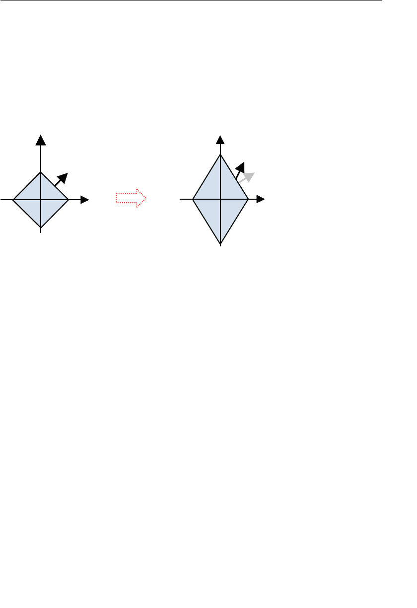
ptg11539634

467

scale(2.0, 2.0, 2.0) . In this situation, even if the size of the object is modified, its

shape is left unchanged. Alternatively, those cases involving a scaling transformation with

a nonuniform scale factor require that you use a different scaling factor for each axis. For

instance, if you limit the scaling to the y-axis direction, you will use

Matrix4.scale(1.0,

2.0,1.0) .

You have to resort to the inverse transpose matrix in case (3) because, if the scaling is

nonuniform, the direction of the normal vector is incorrectly modified when multiplying

it with the model matrix that incorporates the scaling transformation. Figure E.3 shows

this.

direction of normal

(1, 2, 0)

direction of normal

(1, 1, 0)

Scale by 2 along the y-axis

Figure E.3 Simply multiplying the normal vector with the model matrix results in a modification

of the normal direction

Performing a nonuniform scaling of the object (left side of the figure), with a scaling

factor of 2.0 limited to the y-axis, results in the shape on the right. Here, to determine

the normal direction after the transformation, you multiply the model matrix with the

normal (1. 1, 0) of the left side object. However, then the direction of the normal is

changed to (1, 2, 0) and is no longer at a right angle (90 degrees) to the line.

The solution to this requires a little math. We will call the model matrix M , the original

normal n , the transformation matrix M ‘, which transforms n without changing the direc-

tion of n , and the vector perpendicular to n , s . In addition, we define n ‘ and s ‘, as shown

in Equations E.1 and E.2:

Equation E.1 n ‘ = M ‘ × n

Equation E.2 s ‘ = M × s

See Figure E.4 .

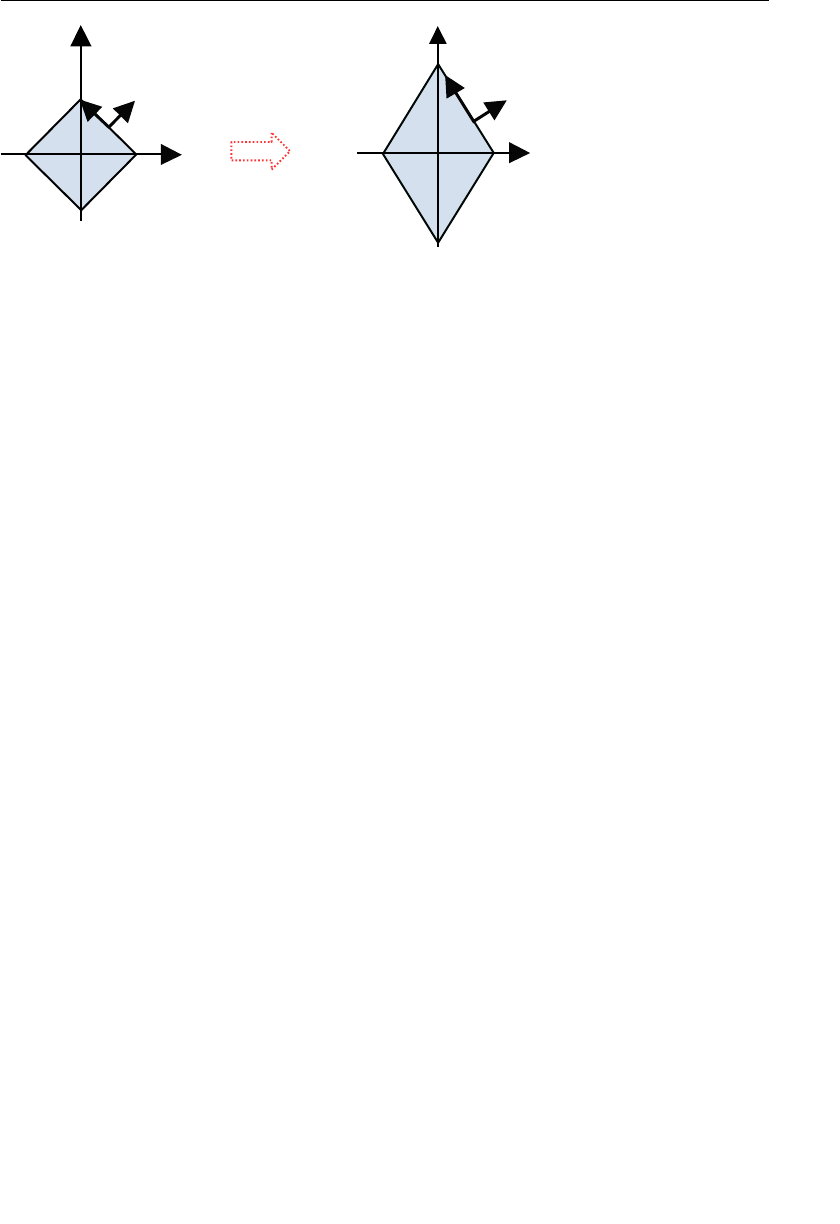
ptg11539634

APPENDIX E The Inverse Transpose Matrix

468

s’

n’

Transformation Matrix: M

Figure E.4 The relationship between n and s, and, n’ and s’.

Here, you can calculate M ‘ so that the two vectors n ‘ and s ‘ form a right angle. If the two

vectors form a right angle, their dot product is equal to 0. Using the “·” notation for a

dot product, you can derive the following equation:

n ’. s ’ = 0

You can now rewrite this expression using the equations E.1 and E.2 ( M

T is the transpose

matrix of M ):

( M ’ × n ) · ( M × s ) = 0

( M ’ × n )

× ( M × s ) = 0 A . B = A

× B

× M ’

× M × s = 0 ( A × B )

= B

× A

Because n and s form a right angle, their dot product is also 0 ( n s = 0). Therefore, as

already stated, A

. B = A

× B , so substituting n for A and s for B will result in n

. s = n

× s

= 0. Comparing this expression with the equation E.3, if the goal is for the products M ‘

× M

between n

T and s to be equal to the identity matrix ( I ), this can be reformulated as

follows:

M ’

× M

= I

Resolving this equation provides us with the following result ( M

–1 is the inverse matrix of

M ):

M ’ = ( M

–1

)

From this equation, you can see that M ‘ is the transpose matrix of the inverse matrix of

M or, in other words, the inverse transpose of M . Because M can include cases (1), (2),

and (3) enumerated earlier, if you calculate the inverse transpose matrix of M and multi-

ply it with the normal vector, you will get the correct result. Thus, this provides the solu-

tion for transforming the normal vector.

ptg11539634

469

Obviously, the calculation of the inverse transpose matrix can be time consuming, but if

you can confirm the model matrix fits criteria (1) or (2), you can simply use the 3×3 sub-

matrix for increased efficiency.

ptg11539634

This page intentionally left blank

ptg11539634

Appendix F

Load Shader Programs from Files

All the sample programs in this book embed the shader programs in the JavaScript

program, which increases the readability of the sample programs but makes it hard to

construct and maintain the shader programs.

As an alternative, you can load the shader programs from files by using the same

methods described in the section “Load and Display 3D Models” in Chapter 10 ,

“Advanced Techniques.” To see how that’s done, let’s modify

ColoredTriangle from

Chapter 5 , “Using Colors and Texture Images,” to add support for loading shaders from

a file. The new program is called

LoadShaderFromFiles , which is shown in Listing F.1 .

Listing F.1 LoadShaderFromFiles

1 // LoadShaderFromFiles.js based on ColoredTriangle.js

2 // Vertex shader program

3 var VSHADER_SOURCE = null;

4 // Fragment shader program

5 var FSHADER_SOURCE = null;

7 function main() {

8 // Retrieve <canvas> element

9 var canvas = document.getElementById(‘webgl’);

11 // Get the rendering context for WebGL

12 var gl = getWebGLContext(canvas);

…

17 // Load the shaders from files

18 loadShaderFile(gl, ‘ColoredTriangle.vert’, gl.VERTEX_SHADER);

19 loadShaderFile(gl, ‘ColoredTriangle.frag’, gl.FRAGMENT_SHADER);

20 }

ptg11539634

APPENDIX F Load Shader Programs from Files

472

22 function start(gl) {

23 // Initialize shaders

24 if (!initShaders(gl, VSHADER_SOURCE, FSHADER_SOURCE)) {

…

43 gl.drawArrays(gl.TRIANGLES, 0, n);

44 }

…

88 function loadShaderFile(gl, fileName, shader) {

89 var request = new XMLHttpRequest();

91 request.onreadystatechange = function() {

92 if (request.readyState === 4 && request.status !== 404) {

93 onLoadShader(gl, request.responseText, shader);

94 }

95 }

96 request.open(‘GET’, fileName, true);

97 request.send(); // Send the request

98 }

100 function onLoadShader(gl, fileString, type) {

101 if (type == gl.VERTEX_SHADER) { // The vertex shader is loaded

102 VSHADER_SOURCE = fileString;

103 } else

104 if (type == gl.FRAGMENT_SHADER) { // The fragment shader is loaded

105 FSHADER_SOURCE = fileString;

106 }

107 // Start rendering, after loading both shaders

108 if (VSHADER_SOURCE && FSHADER_SOURCE) start(gl);

109 }

Unlike ColoredTriangle.js , this sample program initializes the VSHADER_PROGRAM (line

3) and

FSHADER_PROGRAM (line 5) to null to allow them to be loaded from files later. The

function

main() defined at line 7 loads the shader programs at lines 18 and line 19 by

using

loadShaderFile() . This function is defined at line 88, and its second argument

specifies the filename (URL) that contains the shader program. The third argument speci-

fies the type of the shader program.

The function

loadShaderFile() creates a request of type XMLHttpRequest to get the file

specified by fileName and then registers an event handler (

onLoadShader() ) at line 91 to

handle the file when it is loaded. After that, it sends the request at line 97. Once the file is

acquired,

onLoadShader() is called. This function is defined at line 100.

The onLoadShader() checks the third parameter type and uses it to store the fileString

containing the shader program to

VSHADER_PROGRAM or FSHADER_PROGRAM . Once you load

both shader programs, call

start(gl) at line 108 to draw the triangle using the shaders.

ptg11539634

Appendix G

World Coordinate System Versus Local

Coordinate System

In Chapter 7 , “Toward the 3D World,” you used and displayed your first 3D object

(a cube), allowing the sample program to begin to feel more like a “real” 3D applica-

tion. However, to do so, you had to manually set up the vertex coordinates and the

index information of the cube, which was quite time consuming. Although you will

do the same manual setup throughout this book, this is not something you will gener-

ally do when creating your own WebGL applications. Usually you will use a dedicated

3D modeling tool to create 3D objects. This allows you to create elaborate 3D objects

through the manipulation (combination, deformation, vertex population adjustment,

vertex interval tuning, and so on) of elementary 3D shapes, such as cubes, cylinders, or

spheres. The 3D modeling tool Blender ( www.blender.org/ ) is shown in Figure G.1 .

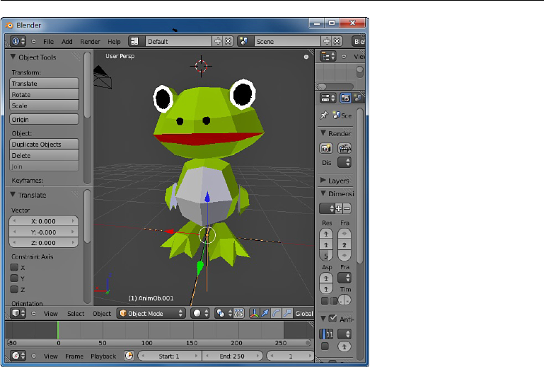
ptg11539634

APPENDIX G World Coordinate System Versus Local Coordinate System

474

Figure G.1 Creation of a 3D object with a 3D modeling tool

The Local Coordinate System

When creating the model of a 3D object, it is necessary to decide where the origin (that

is, (0, 0, 0)) is placed for the model. You can choose the origin of the model so that the

model can be easily built, or alternatively so that the created model can be handled easily

in a 3D scene. The cube introduced in the previous section was created with its center

set at the origin (0, 0, 0). Sphere-shaped objects, like the sun or the moon, are usually

modeled with their center at the origin.

On the other hand, in the case of game character models, such as the one shown in Figure

G.1 , most of the models are built with the origin positioned at their feet level, and the

y-axis running through the center of the body. By doing so, if you place the character at

the y coordinate = 0 height (at the ground level), the character looks like it is standing

on the ground—neither floating above the ground nor sinking down into the ground. In

this configuration, if you translate the model along the z-axis or x-axis, the character will

appear to be walking or gliding along the ground. Additionally, you can turn the character

using a simple rotation around the y-axis.

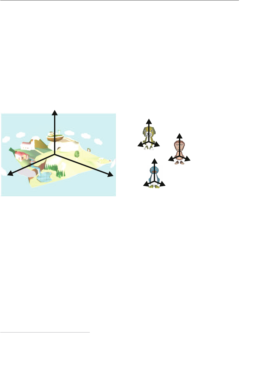
ptg11539634

The World Coordinate System 475

In such cases, the coordinates of the vertices that constitute objects or characters config-

ured in this fashion are expressed with respect to this origin. Such a coordinate system

is called the local coordinate system . Using modeling tools (like Blender), the compo-

nents (vertex coordinates, colors, indices, and so on) of models designed this way can be

exported to a file. You can then import this information into the buffer object in WebGL,

and using

gl.drawElements() , you can draw and display the model created with the 3D

modeling tool.

The World Coordinate System

Let’s consider the case of a game where multiple characters would appear in a single

space. The goal is to use the characters illustrated in Figure G.2 (right side) in the 3D scene

shown on the left side. All three characters and the world have their own origin.

(0, 0, 0)

Figure G.2 Disposition of several characters inside a single world

When you want to display the characters as they are, you are faced with a problem.

Because all the characters are built with their origin positioned at their feet level, they

eventually are displayed on top of each other at the same location: the origin (0, 0, 0) of

the 3D scene ( Figure G.3 ).

1 That’s not something that generally happens in the real world

and certainly not what you want here.

1 To keep the  gure understandable, the characters are placed at slightly shifted positions.

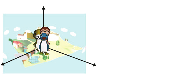
ptg11539634

APPENDIX G World Coordinate System Versus Local Coordinate System

476

(0, 0, 0)

Figure G.3 All the characters are displayed at the origin.

To address this problem, you need to adjust the position of each character to avoid

them overlapping. To achieve this, you can use coordinate transformations that you

originally looked at in Chapter 3 , “Drawing and Transforming Triangles,” and 4, “More

Transformations and Basic Animation.” To prevent the characters from overlapping, you

could translate the penguin to (100, 0, 0), the monkey to (200, 10, 120), and the dog to

(10, 0, 200).

The coordinate system we use to correctly place characters created within a local coor-

dinate system is called the world coordinate system , or alternatively the global

coordinate system . The associated model transformation is referred to as the world

transformation .

Of course, to prevent the characters of the penguin, monkey, and dog from overlapping,

you can build them using the world coordinate system. For example, if you model the

penguin in a tool such as Blender with its origin set to (100, 0, 0), when you insert the

penguin into the world, it will be displayed at position (100, 0, 0), so you don’t need a

coordinate transformation to avoid overlapping. However, this approach creates its own

difficulties. For example, it becomes difficult to make the penguin spin like a ballerina

because, if you perform a rotation around the y-axis, you generate a circular motion of

radius 100. You could, of course, first translate the penguin back to the origin, rotate it,

and then translate it again to the original position, but that is quite a lot of work.

You actually already dealt with a similar case in Chapter 7 . Using the coordinates of one

set of triangles, the vertices of which were determined with respect to the origin set at the

center,

PerspectiveView_mvp draws a second set of triangles. Here is the figure we referred

to in that program (see Figure G.4 ).

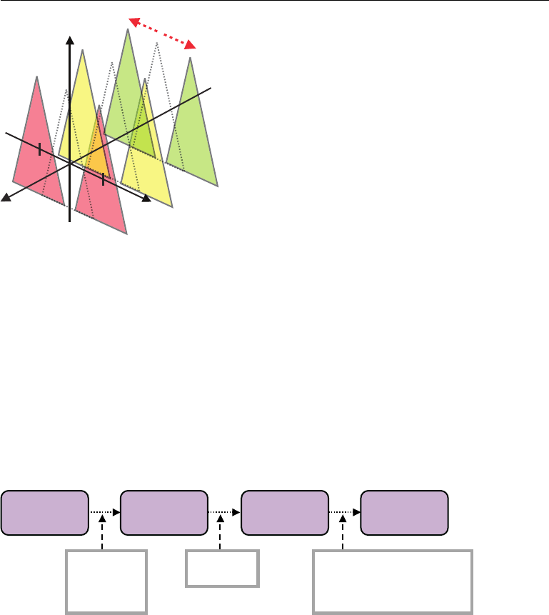
ptg11539634

Transformations and the Coordinate Systems 477

-0.75

0.75 x

Figure G.4 Triangles group in PerspectiveView_mvp

Here, the local coordinate system expresses the vertex coordinates of the triangles shown

with the dotted lines, whereas the world coordinate system is used to describe their trans-

lation along the x-axis.

Transformations and the Coordinate Systems

So far, we have not considered local and world coordinate systems so that you can focus

on the core aspects of each example. However, for reference, Figure G.5 shows the rela-

tionship between the transformations and the coordinate systems and is something to

bear in mind as you deepen your knowledge of 3D graphics and experiment with model-

ing tools.

local

coordinate

system

world

coordinate

system

clipping

coordinate

system

view

coordinate

system

model matrix

translate(),

rotate(),

scale()

view matrix

lookAt()

orthographic projection matrix

setOrtho()

perspective projection matrix

setPerspective()

Figure G.5 Transformation and the coordinate system

ptg11539634

This page intentionally left blank

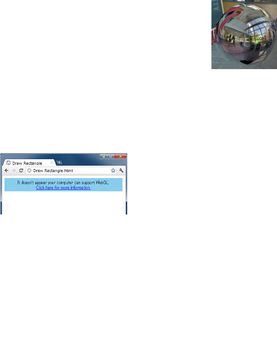
ptg11539634

Appendix H

Web Browser Settings for WebGL

This appendix explains how to use advanced web browser settings to ensure that

WebGL is displayed correctly and what to do if it isn’t.

If your graphics board isn’t compatible with WebGL, you may see the message shown

in Figure H.1 .

Figure H.1 Loading a WebGL application results in an error message

If this happens, you may still be able to get WebGL to work in your browser with a

little bit of tweaking:

1. If you are using Chrome, start the browser with the option

—ignore-gpu-black-

list . To specify this option, right-click the Chrome browser shortcut icon and

select Properties from the menu. You’ll see a pop-up window similar to that in

Figure H.2 . Then add the option string at the end of the command string in the

Target column on the window. After that, Chrome is always started with the

option. If this solves your problem, leave this option enabled.

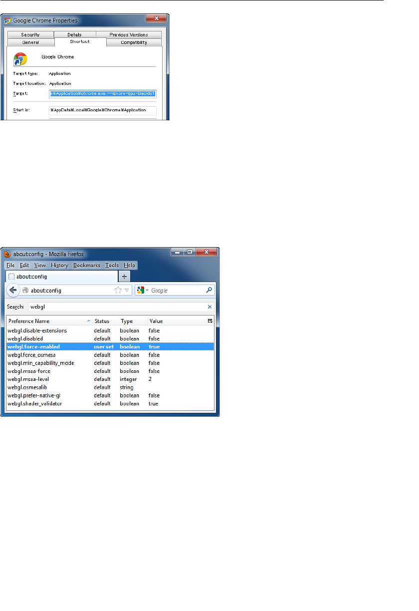
ptg11539634

APPENDIX H Web Browser Settings for WebGL

480

Figure H.2 Specifying an option in the Google Chrome Properties window

2. If you are using Firefox, enter

about:config in the address bar. Firefox shows “This

might void your warranty!” Click the button labeled “I’ll be careful, I promise!” Type

webgl in the text field labeled by Search or Filter, and then Firefox will display the

WebGL-related setting names (see Figure H.3 ). Double-click

webgl.force-enabled in

the list to change its value from

false to true . Again, if this solves your problem,

leave this option enabled.

Figure H.3 WebGL-related settings in Firefox

If neither solution works, you will have to find another machine that has better support

for WebGL. Again, look at the Khronos wiki for more information: www.khronos.org/

webgl/wiki .

ptg11539634

Glossary

alpha blending The process of using the alpha value (“A”) in RGBA to blend the

colors of two or more objects.

alpha value The value used to indicate the transparency (0.0 is transparent and 1.0

is opaque) of an object. Alpha blending uses this value.

ambient light Indirect light. Light that illuminates an object from all directions and

with the same intensity.

attach The process of establishing a connection between two existing objects.

Compare to bind .

attribute variable The variable used to pass data to a vertex shader.

bind The process of creating a new object and then establishing a connection (the

binding) between that object and a rendering context. Compare to attach .

buffer A block of memory allocated and dedicated to storing a speci c kind of data,

such as color or depth values.

buffer object WebGL object used to store multiple items of vertex information.

canvas The HTML5 element and features to draw graphics on a web page.

clipping An operation that identi es the area (or region) within a 3D scene that

will be drawn. Anything not in the clipping region is not drawn.

color buffer The memory area into which WebGL draws. Once drawn, the contents

are displayed on the screen.

column major A convention describing the way a matrix is stored in an array. In

column major, the columns are listed in sequence in the array.

ptg11539634

Glossary

482

completeness Used in the context of a framebuffer, indicates the state whether a frame-

buffer object meets all the requirements for drawing.

context JavaScript object that implements the methods used to draw onto a canvas.

depth (value) The z value of a fragment when viewing the fragment from the eye point

along the line of sight.

depth buffer The memory area used for hidden surface removal. It stores the depth value

(z value) of all fragments.

directional light A light source that emits parallel light rays.

far clipping plane The farther clipping plane of the planes comprising the viewing volume

from the eye point.

fog The effect seen when fading colors to a background color based on the distance from

the observer. Fog is often used to provide depth cues to the observer.

fragment The pixel generated by the rasterization process and which has color, depth

value, texture coordinates, and more.

fragment shader The shader program to process the fragment information.

framebuffer object WebGL object used for offscreen drawing.

GLSL ES OpenGL ES Shading Language. ES stands for Embedded System.

hidden surface removal The process to determine and hide the surfaces and parts of sur-

faces that are not visible from a certain viewpoint.

image A rectangular array of pixels.

index (vertex) See vertex index .

local coordinates The vertex coordinates that are de ned in the local coordinate system

(the coordinate system that relates speci cally to the selected object). (Also see world coordi-

nates. )

ptg11539634

Glossary 483

model matrix The matrix used to translate, rotate, or scale objects. It is also known as a

modeling matrix.

model view matrix The matrix that multiplies the view matrix by the model matrix.

model view projection matrix The matrix that multiplies the projection matrix by the

model view matrix.

near clipping plane The nearer clipping plane of the planes comprising the viewing vol-

ume from the eye point.

normal An imaginary line that is perpendicular to the surface of a polygon and represent-

ed by a vec3 number. It is also called the normal vector.

orthographic projection matrix The matrix used to de ne a box-shaped viewing volume—

left, right, bottom, top, near, far—that de nes the clipping planes of the box. Objects

located closer to the far clipping plane are not scaled.

perspective projection matrix The matrix used to de ne a pyramid-shaped viewing

volume. Objects located closer to the far clipping plane are scaled appropriately to give

perspective.

pixel Picture element. It has an RGBA or RGB value.

point light Light source that emits light in all directions from one point.

program object WebGL object to manage shader objects.

projection matrix The generic term for the orthographic projection matrix and the per-

spective projection matrix.

rasterization process The process to convert shapes, de ned in a vector format into frag-

ments (pixels or dots) for display on a video screen.

renderbuffer object WebGL object that supports a general two-dimensional drawing area.

RGBA A color format: R (red), G (green), B (blue), and A (alpha).

sampler A data type used to access a texture image from within a fragment shader.

shader The computer program that implements the fundamental drawing function used

in WebGL. WebGL supports vertex shaders and fragment shaders.

ptg11539634

Glossary

484

shader object WebGL object to manage shaders.

shading The process of applying shading to each face of an object.

shadowing The process to determine and draw shadows cast by objects.

texel The basic element ( tex ture el ement) that makes up a texture image. It has RGB or

RGBA value.

texture coordinates Two-dimensional coordinates to be used to access a texture image.

texture image The image used in texture mapping. It is also simply called texture.

texture mapping The process of applying (mapping) a texture image to the surface of an

object.

texture object WebGL object to manage a texture image.

texture unit The mechanism to manage multiple texture objects.

transformation The process of converting the vertex coordinates of an object to new vertex

coordinates as a result of applying a transformation (translation, scaling, and so on).

uniform variable The variable used to pass data to the vertex shader or fragment shader.

varying variable The variable used to pass data from the vertex shader to the fragment

shader.

vertex index The number assigned to the vertex information elements stored in a buffer

object. It starts from 0 and is increased by 1 for each new element stored.

vertex shader The shader program that processes the vertex information.

view coordinate system The coordinate system that has the eye point at its origin, the line

of sight along the negative z-axis, and the up direction in the positive y-axis.

view matrix The matrix to transform the vertex coordinates to the coordinates that are

viewed from the eye point toward the line of sight.

view projection matrix The matrix that multiplies the projection matrix by the view ma-

trix.

viewing volume The subspace that is displayed on the screen. The objects outside the vol-

ume are not displayed.

world coordinates The coordinates that are obtained by multiplying the model matrix by

the local vertex coordinates of the 3D model.

ptg11539634

References

Bowman, Doug A., Ernst Kruijff, Joseph J. LaViola Jr, and Ivan Poupyrev. 3D User

Interfaces: Theory and Practice . Addison-Wesley Professional (July 26, 2004).

Dunn, Fletcher, and Ian Parberry. 3D Math Primer for Graphics and Game Development , 2nd

Edition. A K Peters/CRC Press (November 2, 2011).

Foley, James D., Andries van Dam, Steven K. Feiner, and John F. Hughes. Computer

Graphics: Principles and Practice in C , 2nd Edition. Addison-Wesley Professional (August 4,

1995).

Munshi, Aaftab, Dan Ginsburg, and Dave Shreiner. OpenGL ES 2.0 Programming Guide .

Addison-Wesley Professional (July 24, 2008).

Shreiner, Dave. The Khronos OpenGL ARB Working Group. OpenGL Programming Guide:

The Official Guide to Learning OpenGL, Versions 3.0 and 3.1 , 7th Edition. Addison-Wesley

Professional (July 21, 2009).

ptg11539634

This page intentionally left blank

ptg11539634

Index

Symbols

2D graphics

coloring vertices different colors,

151-160

geometric shape assembly and

rasterization, 151-155

invoking fragment shader, 155

varying variables and interpolation

process, 157-160

verifying fragment shader

invocation, 156-157

combining multiple transformations,

119-121

drawing

rectangles, 13-16, 89-91

triangles, 85-91

pasting images on, 160-183

activating texture units, 171-172

assigning texture images to texture

objects, 177-179

binding texture objects to target,

173-174

changing texture coordinates,

182-183

flipping image y-axis, 170-171

mapping texture and vertex

coordinates, 162-163, 166

multiple texture mapping, 183-190

passing texture coordinates from

vertex to fragment shader, 180-181

passing texture unit to fragment

shader, 179-180

retrieving texel color in fragment

shader, 181-182

setting texture object parameters,

174-177

setting up and loading images,

166-170

texture coordinates, explained, 162

TexturedQuad.js, 163-166

restoring clipped parts, 251-253

rotating, 96-102, 107-110, 234-235

RotatingTranslatedTriangle.js, 135-136

RotatingTriangle.js, 126-129

calling drawing function, 129-130

draw() function, 130-131

requestAnimationFrame() function,

131-133

updating rotation angle, 133-135

TranslatedTriangle.js, 92-96

translating, 92-96, 111

ptg11539634

Index

488

3D graphics. See alsoWebGL

alpha blending, 384

applications

browser functionality in, 5

publishing, ease of, 4

writing in text editors, 3-4

displaying on web pages

(3DoverWeb), 372

lighting, 291-293

light sources, 293

reflected light, 294-296

loading, 414-416

modeling tools, 415, 473-475

point light objects, 314-315

shading, 292

3D models

MTL file format, 418

OBJ file format, 417

OBJViewer.js, 419-421

parser code, 423-430

user-defined objects, 422-423

3DoverWeb, 372

[ ] (array indexing) operator, 203-204

. (dot) operator, 201-202

; (semicolon), in GLSL ES, 193

abs() function, 444

access to members

of arrays in GLSL ES, 209

of structures in GLSL ES, 207

of vector and matrix data types,

201-204

acos() function, 442

activating texture units, 171-172

adding

color to each face (Hello Cube),

284-285

shading to ambient light, 307-308

affine transformations, 91

all() function, 450

alpha blending, 380

3D objects, 384

blending function, 382-383

drawing when alpha values coexist,

385-386

implementing, 380-381

LookAtBlendedTriangles.js, 381-382

ambient light, 294

shading, adding, 307-308

ambient reflection, 295-296

angle functions, 216, 441-442

animate() function, 129, 133-135

animation, 124-136

multiple transformations in, 135-136

RotatingTriangle.js, 126-129

calling drawing function, 129-130

draw() function, 130-131

requestAnimationFrame() function,

131-133

updating rotation angle, 133-135

anonymous functions, 52-53

any() function, 450

applications

3D graphics applications

browser functionality in, 5

publishing, ease of, 4

writing in text editors, 3-4

WebGL application structure, 6-7

ptg11539634

Index 489

array indexing ([ ]) operator, 203-204

arrays

in GLSL ES, 208-209

interleaving, 141-145

typed arrays, 78-79

asin() function, 442

assigning

buffer objects to attribute variables,

79-81

texture images to texture objects,

177-179

values

in GLSL ES structures, 207

in GLSL ES variables, 196-197

in matrix data types, 199-201

in vector data types, 199-201

asynchronous loading of texture images,

169-170

atan() function, 442

atmospheric effects, fog, 372-373

attaching shader objects to program

objects, 350-351

attribute variables, 217-218

assiging buffer objects to, 79-81

declaring, 43

enabling assignment, 81-82

explained, 41-42

for point size (MultiAttributeSize.js),

139-140

setting value, 45-49

storage location, 44-45

back color buffer, 437

background objects, 267-269

z fighting, 273-275

binding

buffer objects to targets, 75-76

renderbuffer objects, 399-400

texture objects to targets, 173-174

BlendedCube.js, 384

Blender 3D modeling tool, 415, 473-475

blending function, alpha blending,

382-383

<body> element, 12

bool data type, 196

Boolean values in GLSL ES, 194

boxed-shape viewing volume

defining, 243-244

OrthoView.html, 245-246

OrthoView.js, 246-247

break statement in GLSL ES, 212-213

browsers

<canvas> element support, 12

console, viewing, 14

enabling local file access, 161

functionality in 3D graphics

applications, 5

JavaScript to WebGL processing flow,

27, 438

WebGL settings, 479-480

buffer objects

assigning to attribute variables, 79-81

binding to targets, 75-76

creating, 74-75

ptg11539634

Index

490

creating multiple, 140-141

defined, 69

enabling attribute variable assignment,

81-82

explained, 72-74

writing vertex coordinates, colors, and

indices in, 281-284

writing data to, 76-78

buffers

color buffers, 22

drawing to, 437-439

saving content from, 56

swapping, 437

depth buffer, 22

types of, 22

built-in functions in GLSL ES, 215-216

calculating

color per fragment, 319

diffuse reflection, 297-299

cancelAnimationFrame() function, 133

canvas.addEventListener() function, 432

<canvas> element, 9-11, 243

browser support, 12

clearing drawing area, 16-23

coordinates for center, 23

coordinate system, 16

DrawRectangle.html, 11-13

DrawRectangle.js, 13-16

HelloCanvas.html, 17-18

HelloCanvas.js, 18-23

mapping to WebGL coordinate system,

39, 54-57

retrieving, 14, 19

canvas.getContext() function, 15

case sensitivity of GLSL ES, 193

ceil() function, 444

changing

color with varying variables, 146-151

eye point using keyboard, 238

near value, 250-251

checkFace() function, 368

Chrome

console, viewing, 14

enabling local file access, 161

WebGL browser settings, 479

clamp() function, 445

clear color, setting, 21-23

clearing

color buffer, 22

drawing area, 16-23

ClickedPoints.js, 50-52

clip coordinate system, viewing volume

and, 460-462

clipped parts, restoring, 251-253

color

adding to each face (Hello Cube),

284-285

changing with varying variables,

146-151

of points, changing, 58-66

setting, 15, 21-23

texel color, retrieving in fragment

shader, 181-182

color buffers, 22

drawing to, 437-439

ptg11539634

Index 491

saving content from, 56

swapping, 437

ColoredCube.js, 285-289

ColoredPoints.js, 59-61

ColoredTriangle.js, 159

coloring vertices, 151-160

geometric shape assembly and

rasterization, 151-155

invoking fragment shader, 155

varying variables and interpolation

process, 157-160

verifying fragment shader invocation,

156-157

color per fragment, calculating, 319

column major order, 109-110

combining multiple transformations,

119-121

comments in GLSL ES, 193

common functions, 216, 444-446

compiling shader objects, 347-349

conditional control flow in GLSL ES,

211-213

console, viewing, 14

constant index, 203

constants of typed arrays, 79

constructors in GLSL ES, 199-201

for structures, 207

const variables in GLSL ES, 217

context, retrieving, 15, 20-21

continue statement in GLSL ES, 212-213

coordinates

center of canvas, 23

homogeneous coordinates, 35

for mouse clicks, 54-57

WebGL coordinate system, 38-39

CoordinateSystem.js, 456-459

coordinate systems

for <canvas> element, 16

clip coordinate system and viewing

volume, 460-462

CoordinateSystem.js, 456-459

handedness in default behavior,

455-464

Hidden Surface Removal tool, 459-460

local coordinate system, 474-475

projection matrices for, 462-464

texture coordinates

changing, 182-183

explained, 162

flipping image y-axis, 170-171

mapping to vertex coordinates,

162-163, 166

passing from vertex to fragment

shader, 180-181

transformations and, 477

world coordinate system, 475-477

CoordinateSystem_viewVolume.js, 461

cos() function, 442

createProgram() function, 354

cross() function, 447

ctx.fillRect() function, 16

cubes, 301

cuboids, 301

cuon-matrix.js, 116

cuon-utils.js, 20

ptg11539634

Index

492

data, passing

to fragment shaders with varying

variable, 146-151

to vertex shaders, 137-151. See

alsodrawing; rectangles; shapes;

triangles

color changes, 146-151

creating multiple buffer objects,

140-141

interleaving, 141-145

MultiAttributeSize.js, 139-140

data types

in GLSL ES, 34, 194-196

arrays, 208-209

operators on, 197-198

precision qualifiers, 219-221

samplers, 209-210

structures, 207-208

type conversion, 196-197

type sensitivity, 195

vector and matrix types, 198-206

typed arrays, 78-79

#define preprocessor directive, 222

degrees() function, 441

deleting

shader objects, 346

texture objects, 167

depth buffer, 22

DepthBuffer.js, 272-273

diffuse reflection, 294-295

calculating, 297-299

shading, 296-297

Direct3D, 5

directional light, 293

shading, 296-297

discard statement in GLSL ES, 212-213

displaying 3D objects on web pages

(3DoverWeb), 372

distance() function, 447

document.getElementById() function,

14, 19

dot() function, 447

dot (.) operator, 201-202

draw() function, 129-131

objects composed of other objects,

332-334

processing flow of, 249

drawArrays() function, 284

drawbox() function, 339-340

drawing

to color buffers, 437-439

Hello Cube with indices and vertices

coordinates, 277-278

multiple points/vertices, 68-85

assigning buffer objects to attribute

variables, 79-81

binding buffer objects to targets,

75-76

buffer object usage, 72-74

creating buffer objects, 74-75

enabling attribute variable

assignments, 81-82

gl.drawArrays() function, 82-83

writing data to buffer objects, 76-78

objects composed of other objects,

324-325

points

assigning uniform variable values,

63-66

attribute variables, 41-42

ptg11539634

Index 493

attribute variable storage location,

44-45

attribute variable value, 45-49

changing point color, 58-66

ClickedPoints.js, 50-52

ColoredPoints.js, 59-61

fragment shaders, 35-36

gl.drawArrays() function, 36-37

handling mouse clicks, 53-57

HelloPoint1.html, 25

HelloPoint1.js, 25-26

HelloPoint2.js, 42-43

initializing shaders, 30-33

method one, 23-41

method two, 41-50

with mouse clicks, 50-58

registering event handlers, 52-53

shaders, explained, 27-28

uniform variables, 61-62

uniform variable storage location,

62-63

vertex shaders, 33-35

WebGL coordinate system, 38-39

WebGL program structure, 28-30

rectangles, 13-16, 89-91

shapes, 85-91

animation, 124-136

multiple vertices, 68-85

rotating, 96-110

scaling, 111-113

transformation libraries, 115-124

translating, 92-96, 105-106, 111

triangles, 85-81

coloring vertices different colors,

151-160

combining multiple

transformations, 119-121

HelloTriangle.js, 85-86

restoring clipped parts, 251-253

rotating, 96-102, 107-110, 234-235

RotatingTranslatedTriangle.js,

135-136

RotatingTriangle.js, 126-135

TranslatedTriangle.js, 92-96

translating, 92-96, 111

using framebuffer objects, 403-404

when alpha values coexist, 385-386

drawing area

clearing, 16-23

defining, 12

mapping to WebGL coordinate

system, 39

drawing context. Seecontext, retrieving

drawing function (tick()), calling

repeatedly, 129-130

DrawRectangle.html, 11-13

DrawRectangle.js, 13-16

drawSegment() function, 340

draw segments, objects composed of other

objects, 339-344

dynamic web pages, WebGL web pages

versus, 7

#else preprocessor directive, 222

enabling

attribute variable assignment, 81-82

local file access, 161

equal() function, 450

event handlers

for mouse clicks, 53-57

registering, 52-53

ptg11539634

Index

494

execution order in GLSL ES, 193

exp2() function, 443

exp() function, 443

exponential functions, 216, 443

eye point, 228

changing using keyboard, 238

LookAtTrianglesWithKeys.js, 238-241

visible range, 241

faceforward() function, 447

face of objects, selecting, 365

PickFace.js, 366-368

files, loading shader programs from,

471-472

fill color, setting, 15

Firefox

console, viewing, 14

enabling local file access, 161

WebGL browser settings, 480

flipping image y-axis, 170-171

Float32Array object, 78

float data type, 196

floor() function, 444

flow of vertex shaders, processing,

248-249

fog, 372-373

implementing, 373-374

w value, 376-377

Fog.js, 374-376

Fog_w.js, 376-377

foreground objects, 267-269

DepthBuffer.js, 272-273

hidden surface removal, 270-271

z fighting, 273-275

for statement in GLSL ES, 211-212

fract() function, 444

fragments, 27, 35

fragment shaders, 27

drawing points, 35-36

example of, 192

geometric shape assembly and

rasterization, 151-155

invoking, 155

passing

data to, 61-62, 146-151

texture coordinates to, 180-181

texture units to, 179-180

program structure, 29-30

retrieving texel color in, 181-182

varying variables and interpolation

process, 157-160

verifying invocation, 156-157

FramebufferObject.js, 395-396, 403

framebuffer objects, 392-393

checking configurations, 402-403

creating, 397

drawing with, 403-404

renderbuffer objects set to, 401-402

setting to renderbuffer objects, 400-401

front color buffer, 437

functions

abs() function, 444

acos() function, 442

ptg11539634

Index 495

all() function, 450

angle and trigonometry functions,

441-442

animate() function, 129, 133-135

anonymous functions, 52-53

any() function, 450

asin() function, 442

atan() function, 442

built-in functions in GLSL ES, 215-216

cancelAnimationFrame() function, 133

canvas.addEventListener()

function, 432

canvas.getContext() function, 15

ceil() function, 444

checkFace() function, 368

clamp() function, 445

common functions, 444-446

cos() function, 442

createProgram() function, 354

cross() function, 447

ctx.fillRect() function, 16

degrees() function, 441

distance() function, 447

document.getElementById() function,

14, 19

dot() function, 447

draw() function, 129-131

objects composed of other objects,

332-334

processing flow of, 249

drawArrays() function, 284

drawbox() function, 339-340

drawSegment() function, 340

equal() function, 450

exp2() function, 443

exp() function, 443

exponential functions, 216, 443

faceforward() function, 447

floor() function, 444

fract() function, 444

geometric functions, 216, 447-448

getWebGLContext() function, 20

gl.activeTexture() function, 171-172

gl.attachShader() function, 350

gl.bindBuffer() function, 75-76

gl.bindFramebuffer() function, 400

gl.bindRenderbuffer() function, 399

gl.bindTexture() function, 173-174

gl.blendFunc() function, 382-383

gl.bufferData() function, 76-78

gl.checkFramebufferStatus() function,

402-403

gl.clearColor() function, 20-21

gl.clear() function, 22, 125

gl.compileShader() function, 347-349

gl.createBuffer() function, 74-75

gl.createFramebuffer() function, 397

gl.createProgram() function, 349-350

gl.createRenderbuffer() function, 398

gl.createShader() function, 345-346

gl.createTexture() function, 167

gl.deleteBuffer() function, 75

gl.deleteFramebuffer() function, 397

gl.deleteProgram() function, 350

gl.deleteRenderbuffer() function, 398

gl.deleteShader() function, 346

gl.deleteTexture() function, 167

ptg11539634

Index

496

gl.depthMask() function, 385

gl.detachShader() function, 351

gl.disable() function, 271

gl.disableVertexAttribArray()

function, 82

gl.drawArrays() function, 36-37, 72,

82-83, 87, 131

gl.drawElements() function, 278

gl.enable() function, 270

gl.enableVertexAttribArray() function,

81-82

gl.framebufferRenderbuffer() function,

401-402

gl.framebufferTexture2D()

function, 401

gl.getAttribLocation() function, 44-45

gl.getProgramInfoLog() function, 352

gl.getProgramParameter() function, 352

gl.getShaderInfoLog() function, 348

gl.getShaderParameter() function, 348

gl.getUniformLocation() function, 63

gl.linkProgram() function, 351-352

gl.pixelStorei() function, 171

gl.polygonOffset() function, 274

gl.readPixels() function, 364

gl.renderbufferStorage() function, 399

gl.shaderSource() function, 346-347

gl.texImage2D() function, 177-179, 398

gl.texParameteri() function, 174-177

glTranslatef() function, 116

gl.uniform1f() function, 65-66

gl.uniform1i() function, 179-180

gl.uniform2f() function, 65-66

gl.uniform3f() function, 65-66

gl.uniform4f() function, 63-66, 95

gl.uniformMatrix4fv() function, 110

gl.useProgram() function, 353, 387

gl.vertexAttrib1f() function, 47-49

gl.vertexAttrib2f() function, 47-49

gl.vertexAttrib3f() function, 45-49

gl.vertexAttrib4f() function, 47-49

gl.vertexAttribPointer() function, 79-81,

142-145

gl.viewport() function, 404

in GLSL ES, 213-215

built-in functions, 215-216

parameter qualifiers, 214-215

prototype declarations, 214

greaterThanEqual() function, 449

greaterThan() function, 449

initShaders() function, 31-32, 344-345,

353-355, 387

initTextures() function, 166-170, 187

initVertexBuffers() function, 72, 140,

152, 166, 187, 281

inversesqrt() function, 443

length() function, 447

lessThanEqual() function, 449

lessThan() function, 449

loadShader() function, 355

loadShaderFile() function, 472

loadTexture() function, 168, 170,

187-189

log() function, 443

log2() function, 443

main() function, processing flow of, 19

mathematical common functions,

444-446

Matrix4.setOrtho() function, 453

Matrix4.setPerspective() function, 453

matrix functions, 216, 448

max() function, 445

ptg11539634

Index 497

maxtrixCompMult() function, 448

min() function, 445

mix() function, 446

mod() function, 444

normalize() function, 447

notEqual() function, 450

not() function, 450

onLoadShader() function, 472

OpenGL functions, naming

conventions, 48-49

popMatrix() function, 338

pow() function, 443

pushMatrix() function, 338

radians() function, 441

reflect() function, 448

refract() function, 448

requestAnimationFrame() function,

130-133

setInterval() function, 131

setLookAt() function, 228-229

setOrtho() function, 243

setPerspective() function, 257

setRotate() function, 117, 131

sign() function, 444

sin() function, 442

smoothstep() function, 446

sqrt() function, 443

stencil buffer, 22

step() function, 446

tan() function, 442

texture lookup functions, 451

texture2D() function, 181-182, 451

texture2DLod() function, 451

texture2DProj() function, 451

texture2DProjLod() function, 451

textureCube() function, 451

textureCubeLod() function, 451

tick() function, 129-130

trigonometry functions, 216, 441-442

type conversion, 197

vec4() function, 34-35

vector functions, 48, 216, 449

geometric functions, 216, 447-448

geometric shape assembly, 151-155

getWebGLContext() function, 20

gl.activeTexture() function, 171-172

gl.attachShader() function, 350

gl.bindBuffer() function, 75-76

gl.bindFramebuffer() function, 400

gl.bindRenderbuffer() function, 399

gl.bindTexture() function, 173-174

gl.blendFunc() function, 382-383

gl.bufferData() function, 76-78

gl.checkFramebufferStatus() function,

402-403

gl.clearColor() function, 20-21

gl.clear() function, 22, 125

gl.compileShader() function, 347-349

gl.createBuffer() function, 74-75

gl.createFramebuffer() function, 397

gl.createProgram() function, 349-350

gl.createRenderbuffer() function, 398

gl.createShader() function, 345-346

gl.createTexture() function, 167

gl.deleteBuffer() function, 75

gl.deleteFramebuffer() function, 397

ptg11539634

Index

498

gl.deleteProgram() function, 350

gl.deleteRenderbuffer() function, 398

gl.deleteShader() function, 346

gl.deleteTexture() function, 167

gl.depthMask() function, 385

gl.detachShader() function, 351

gl.disable() function, 271

gl.disableVertexAttribArray() function, 82

gl.drawArrays() function, 36-37, 72, 82-83,

87, 131

gl.drawElements() function, 278

gl.enable() function, 270

gl.enableVertexAttribArray() function,

81-82

gl.framebufferRenderbuffer() function,

401-402

gl.framebufferTexture2D() function, 401

gl.getAttribLocation() function, 44-45

gl.getProgramInfoLog() function, 352

gl.getProgramParameter() function, 352

gl.getShaderInfoLog() function, 348

gl.getShaderParameter() function, 348

gl.getUniformLocation() function, 63

gl.linkProgram() function, 351-352

global coordinate system. Seeworld

coordinate system

global variables in GLSL ES, 216

gl.pixelStorei() function, 171

gl.polygonOffset() function, 274

gl.readPixels() function, 364

gl.renderbufferStorage() function, 399

gl.shaderSource() function, 346-347

GLSL ES (OpenGL ES shading language),

6, 30

case sensitivity, 193

comments, 193

conditional control flow and iteration,

211-213

data types, 34, 194

arrays, 208-209

precision qualifiers, 219-221

samplers, 209-210

structures, 207-208

vector and matrix types, 198-206

functions, 213-215

built-in functions, 215-216

parameter qualifiers, 214-215

prototype declarations, 214

order of execution, 193

overview of, 192

preprocessor directives, 221-223

semicolon (;) usage, 193

variables

assignment of values, 196-197

data types for, 196

global and local variables, 216

keywords and reserved words,

194-195

naming conventions, 194

operator precedence, 210

operators on, 197-198

storage qualifiers, 217-219

type conversion, 196-197

type sensitivity, 195

GLSL (OpenGL shading language), 6

gl.texImage2D() function, 177-179, 398

gl.texParameteri() function, 174-177

glTranslatef() function, 116

gl.uniform1f() function, 65-66

gl.uniform1i() function, 179-180

ptg11539634

Index 499

gl.uniform2f() function, 65-66

gl.uniform3f() function, 65-66

gl.uniform4f() function, 63-66, 95

gl.uniformMatrix4fv() function, 110

gl.useProgram() function, 353, 387

gl.vertexAttrib1f() function, 47-49

gl.vertexAttrib2f() function, 47-49

gl.vertexAttrib3f() function, 45-49

gl.vertexAttrib4f() function, 47-49

gl.vertexAttribPointer() function, 79-81,

142-145

gl.viewport() function, 404

greaterThanEqual() function, 449

greaterThan() function, 449

handedness of coordinate systems,

455-464

clip coordinate system and viewing

volume, 460-462

CoordinateSystem.js, 456-459

Hidden Surface Removal tool, 459-460

projection matrices for, 462-464

Head Up Display (HUD), 368

HUD.html, 369-370

HUD.js, 370-372

implementing, 369

HelloCanvas.html, 17-18

HelloCanvas.js, 18-23

Hello Cube, 275-277

adding color to each face, 284-285

ColoredCube.js, 285-289

drawing with indices and vertices

coordinates, 277-278

HelloCube.js, 278-281

writing vertex coordinates, colors, and

indices in the buffer object, 281-284

HelloCube.js, 278-281

HelloPoint1.html, 25

HelloPoint1.js, 25-26

HelloPoint2.js, 42-43

HelloQuad.js, 89-91

HelloTriangle.js, 85-86, 151-152

hidden surface removal, 270-271, 459-460

hierarchical structure, 325-326

highp precision qualifier, 220

homogeneous coordinates, 35

HTML5

<body> element, 12

<canvas> element, 9-11

browser support, 12

clearing drawing area, 16-23

coordinates for center, 23

coordinate system, 16

DrawRectangle.html, 11-13

DrawRectangle.js, 13-16

HelloCanvas.html, 17-18

HelloCanvas.js, 18-23

mapping to WebGL coordinate

system, 39, 54-57

retrieving, 14, 19

defined, 2

elements, modifying using JavaScript,

247-248

<img> element, 9

ptg11539634

Index

500

HUD (Head Up Display), 368

HUD.html, 369-370

HUD.js, 370-372

implementing, 369

HUD.html, 369-370

HUD.js, 370-372

identifiers, assigning, 12

identity matrix, 119

handedness of coordinate systems,

462-463

if-else statement in GLSL ES, 211

if statement in GLSL ES, 211

images, pasting on rectangles, 160-183

activating texture units, 171-172

assigning texture images to texture

objects, 177-179

binding texture objects to target,

173-174

changing texture coordinates, 182-183

flipping image y-axis, 170-171

mapping texture and vertex

coordinates, 162-163, 166

multiple texture mapping, 183-190

passing coordinates from vertex to

fragment shader, 180-181

passing texture unit to fragment

shader, 179-180

retrieving texel color in fragment

shader, 181-182

setting texture object parameters,

174-177

setting up and loading images, 166-170

texture coordinates, explained, 162

TexturedQuad.js, 163-166

<img> element, 9

implementing

alpha blending, 380-381

fog, 373-374

HUD, 369

lost context, 431-432

object rotation, 358

object selection, 361-362

rounded points, 377-378

shadows, 405-406

switching shaders, 387

texture images, 394

indices, 282

infinity in homogenous coordinates, 35

initializing shaders, 30-33

initShaders() function, 31-32, 344-345,

353-355, 387

initTextures() function, 166-170, 187

initVertexBuffers() function, 72, 140, 152,

166, 187, 281

int data type, 196

integral constant expression, 208

interleaving, 141-145

interpolation process, varying variables

and, 157-160

inversesqrt() function, 443

inverse transpose matrix, 311-312,

465-469

iteration in GLSL ES, 211-213

ptg11539634

Index 501

J–K

JavaScript

drawing area, mapping to WebGL

coordinate system, 39

HTML elements, modifying, 247-248

loading, 12

processing flow into WebGL, 27, 438

JointModel.js, 328-332

joints, 325

JointModel.js, 328-332

multijoint model, 334

MultiJointModel.js, 335-338

single joint model, objects composed

of other objects, 326-327

keyboard, changing eye point, 238

keywords in GLSL ES, 194-195

Khronos Group, 6

left-handedness of coordinate systems in

default behavior, 455-464

length() function, 447

lessThanEqual() function, 449

lessThan() function, 449

libraries, transformation, 115-124

combining multiple transformations,

119-121

cuon-matrix.js, 116

RotatedTranslatedTriangle.js, 121-124

RotatedTriangle_Matrix4.js, 117-119

light direction, calculating diffuse

reflection, 297-299

LightedCube_ambient.js, 308-309

LightedCube.js, 302-303

processing in JavaScript, 306

processing in vertex shader, 304-305

LightedTranslatedRotatedCube.js, 312-314

lighting

3D objects, 291-293

light sources, 293

reflected light, 294-296

ambient light, 294

directional light, 293

point light, 293

reflected light, 294-296

translated-rotated objects, 310-311

light sources, 293

linking program objects, 351-352

listings

array with multiple vertex information

items, 141

BlendedCube.js, 384

ClickedPoints.js, 51-52

ColoredCube.js, 286-287

ColoredPoints.js, 59-61

ColoredTriangle.js, 159

CoordinateSystem.js, 456-458

CoordinateSystem_viewVolume.js, 461

createProgram(), 354

DepthBuffer.js, 272-273

drawing multiple points, 69

DrawRectangle.html, 11

DrawRectangle.js, 13-14

Fog.js, 374-375

Fog_w.js, 376-377

fragment shader example, 192

ptg11539634

Index

502

FramebufferObject.js

Processes for Steps 1 to 7, 395-396

Process for Step 8, 403-404

HelloCanvas.html, 18

HelloCanvas.js, 18-19

HelloCube.js, 279-280

HelloPoint1.html, 25

HelloPoint1.js, 26

HelloPoint2.js, 42-43

HelloTriangle.js, 85-86

code snippet, 151-152

HUD.html, 369

HUD.js, 370-371

initShaders(), 353-354

JointModel.js, 328-330

LightedCube_ambient.js, 308-309

LightedCube.js, 302-303

LightedTranslatedRotatedCube.js,

312-313

loadShader(), 355

LoadShaderFromFiles, 471-472

LookAtBlenderTriangles.js, 381-382

LookAtRotatedTriangles.js, 235-236

LookAtRotatedTriangles_mvMatrix.js,

237

LookAtTriangles.js, 229-231

LookAtTrianglesWithKeys.js, 239-240

LookAtTrianglesWithKeys_View

Volume.js, 252-253

MultiAttributeColor.js, 147-148

MultiAttributeSize_Interleaved.js,

142-143

MultiAttributeSize.js, 139-140

MultiJointModel.js

drawing the hierarchy structure,

336-337

key processing, 335-336

MultiJointModel_segment.js, 340-342

MultiPoint.js, 70-72

MultiTexture.js, 185-186

OBJViewer.js, 419-420

onReadComplete(), 428

parser part, 424-426

retrieving the drawing information,

428-429

OrthoView.html, 245-246

OrthoView.js, 246-247

PerspectiveView.js, 258-259

PerspectiveView_mvp.js, 263-265

PickFace.js, 366-367

PickObject.js, 362-363

PointLightedCube.js, 316-317

PointLightedCube_perFragment.js,

319-320

ProgramObject.js

Processes for Steps 1 to 4, 387-389

Processes for Steps 5 through 10,

390-391

RotatedTranslatedTriangle.js, 122

RotatedTriangle.js, 99-100

RotatedTriangle_Matrix4.html, 116

RotatedTriangle_Matrix.js, 107-108

RotateObject.js, 358-359

RotatingTriangle_contextLost.js,

433-434

RotatingTriangle.js, 126-128

RoundedPoint.js, 379

ptg11539634

Index 503

Shadow_highp.js, 413-414

Shadow.js

JavaScript part, 410-411

Shader part, 406-407

TexturedQuad.js, 163-165

TranslatedTriangle.js, 93-94

vertex shader example, 192

Zfighting.js, 274-275

3D objects, 414-416

images for texture mapping, 166-170

JavaScript, 12

shader programs from files, 471-472

loadShader() function, 355

loadShaderFile() function, 472

loadTexture() function, 168, 170, 187-189

local coordinate system, 474-475

local file access, enabling, 161

local variables in GLSL ES, 216

log() function, 443

log2() function, 443

LookAtBlendedTriangles.js, 381-382

look-at point, 228

LookAtRotatedTriangles.js, 235-238

LookAtRotatedTriangles_mvMatrix.js, 237

LookAtTriangles.js, 229-233

LookAtTrianglesWithKeys.js, 238-241

LookAtTrianglesWithKeys_ViewVolume.js,

251-253

lost context, 430-431

implementing, 431-432

RotatingTriangle_contextLost.js,

432-434

lowp precision qualifier, 220

luminance, 178

Mach band, 409

macros, predefined names, 222

main() function, processing flow of, 19

manipulating objects composed of other

objects, 324-325

mapping textures, 160-183

activating texture units, 171-172

assigning texture images to texture

objects, 177-179

binding texture objects to target,

173-174

changing texture coordinates, 182-183

flipping image y-axis, 170-171

mapping vertex and texture

coordinates, 162-163, 166

passing coordinates from vertex to

fragment shader, 180-181

passing texture unit to fragment

shader, 179-180

pasting multiple textures, 183-190

retrieving texel color in fragment

shader, 181-182

setting texture object parameters,

174-177

setting up and loading images, 166-170

texture coordinates, explained, 162

TexturedQuad.js, 163-166

mathematical common functions,

444-446

matrices

defined, 103

identity matrix, 119

handedness of coordinate systems,

462-463

ptg11539634

Index

504

inverse transpose matrix, 311-312,

465-469

model matrix, 121

PerspectiveView, 262, 265

multiplication, 103, 121, 205-206

projection matrix

handedness of coordinate systems,

462-464

quadrangular pryamid, 260-261

Matrix4 object, supported methods and

properties, 118

Matrix4.setOrtho() function, 453

Matrix4.setPerspective() function, 453

matrix data types in GLSL ES, 198-206

access to components, 201-204

assignment of values, 199-201

constructors, 199-201

operators, 204-206

matrix functions, 216, 448

max() function, 445

maxtrixCompMult() function, 448

mediump precision qualifier, 220

member access in GLSL ES

arrays, 209

structures, 207

methods. See alsofunctions

for Matrix4 object, 118

of typed arrays, 79

WebGL methods, naming conventions,

48-49

min() function, 445

MIPMAP texture format, 176

mix() function, 446

model matrix, 121

PerspectiveView, 262, 265

model transformation, 121

mod() function, 444

modifying HTML elements using

JavaScript, 247-248

mouse

drawing points, 50-58

ClickedPoints.js, 50-52

event handling, 53-57

registering event handlers, 52-53

rotating objects, 357

moving shapes, 92-96

MTL file format (3D models), 418

MultiAttributeColor.js, 147-150

MultiAttributeSize_Interleaved.js, 142-145

MultiAttributeSize.js, 139-140

multijoint model

MultiJointModel.js, 335-338

objects composed of other objects, 334

MultiJointModel.js, 335-338

MultiJointMode_segment.js, 340-342

multiple buffer objects, creating, 140-141

multiple points, drawing, 68-85

multiple textures, mapping to shapes,

183-190

multiple transformations, 115-124

in animation, 135-136

combining, 119-121

cuon-matrix.js, 116

RotatedTranslatedTriangle.js, 121-124

RotatedTriangle_Matrix4.js, 117-119

multiple vertices

basic shapes, drawing, 85-91

drawing, 68-85

assigning buffer objects to attribute

variables, 79-81

binding buffer objects to targets,

75-76

ptg11539634

Index 505

buffer object usage, 72-74

creating buffer objects, 74-75

enabling attribute variable

assignments, 81-82

gl.drawArrays() function, 82-83

writing data to buffer objects, 76-78

multiplication

of matrices, 121

of vectors and matrices, 103, 205-206

MultiPoint.js, 70-72

MultiTexture.js, 184-190

naming conventions

GLSL ES variables, 194

variables, 43

WebGL methods, 48-49

near value, changing, 250-251

normal orientation of a surface, 299-301

normalize() function, 447

notEqual() function, 450

not() function, 450

numerical values in GLSL ES, 194

objects

composed of other objects

draw() function, 332-334

drawing, 324-325

draw segments, 339-344

hierarchical structure, 325-326

JointModel.js, 328-332

manipulating, 324-325

multijoint model, 334

single joint model, 326-327

rotation

implementing, 358

with mouse, 357

RotateObject.js, 358-360

selection, 360-362

face of objects, 365

implementing, 361-362

PickObject.js, 362-365

OBJ file format (3D models), 417

OBJViewer.js, 419-421

parser code, 423-430

onLoadShader() function, 472

OpenGL

color buffers, swapping, 437

functions, naming conventions, 48-49

in history of WebGL, 5

WebGL and, 5

OpenGL ES (Embedded Systems), 5-6, 30

OpenGL shading language (GLSL), 6

operator precedence in GLSL ES, 210

operators in GLSL ES

on arrays, 209

on structures, 208

on variables, 197-198

on vector and matrix data types,

204-206

order of execution in GLSL ES, 193

orientation of a surface

calculating diffuse reflection, 297-299

normal, 299-301

ptg11539634

Index

506

origin

in coordinate systems, 55

in local coordinate system, 474-475

in world coordinate system, 475-477

origins of WebGL, 5-6

orthographic projection matrix, 252-253,

261, 453

OrthoView.html, 245-246

OrthoView.js, 246-247

parameter qualifiers in GLSL ES functions,

214-215

parameters of texture objects, setting,

174-177

parser code (OBJViewer.js), 423-430

passing data

to fragment shaders

texture units, 179-180

with varying variable, 146-151

to vertex shaders, 137-151. See

alsodrawing; rectangles; shapes;

triangles

color changes, 146-151

creating multiple buffer objects,

140-141

interleaving, 141-145

MultiAttributeSize.js, 139-140

pasting images on rectangles, 160-183

activating texture units, 171-172

assigning texture images to texture

objects, 177-179

binding texture objects to target,

173-174

changing texture coordinates, 182-183

flipping image y-axis, 170-171

mapping texture and vertex

coordinates, 162-163, 166

multiple texture mapping, 183-190

passing coordinates from vertex to

fragment shader, 180-181

passing texture unit to fragment

shader, 179-180

retrieving texel color in fragment

shader, 181-182

setting texture object parameters,

174-177

setting up and loading images, 166-170

texture coordinates, explained, 162

TexturedQuad.js, 163-166

perspective projection matrix, 257, 453

PerspectiveView.js, 255, 260-263

model matrix, 262, 265

PerspectiveView_mvp.js, 263-266

per-vertex operations, 93

PickFace.js, 365-368

PickObject.js, 362-365

point light, 293

point light objects, 314-315

PointLightedCube.js, 315-319

PointLightedCube_perFragment.js,

319-321

points, drawing, 23-50

attribute variables, 41-42

setting value, 45-49

storage location, 44-45

changing point color, 58-66

ClickedPoints.js, 50-52

ColoredPoints.js, 59-61

gl.drawArrays() function, 36-37

HelloPoint1.html, 25

ptg11539634

Index 507

HelloPoint1.js, 25-26

HelloPoint2.js, 42-43

with mouse clicks, 50-58

multiple points, 68-85

registering event handlers, 52-53

shaders

explained, 27-28

fragment shaders, 35-36

initializing, 30-33

vertex shaders, 33-35

uniform variables, 61-62

assigning values, 63-66

storage location, 62-63

WebGL coordinate system 38-39

WebGL program structure, 28-30

point size, attribute variables for, 139-140

popMatrix() function, 338

positive rotation, 96

pow() function, 443

precedence of operators in GLSL ES, 210

precision qualifiers, 62, 219-221

predefined single parameters, 53

preprocessor directives in GLSL ES,

221-223

primitive assembly process. Seegeometric

shape assembly

primitives. Seeshapes

process flow

initializing shaders, 31

InitShaders() function, 353-355

JavaScript to WebGL, 27, 438

mouse click event handling, 53-57

multiple vertice drawing, 70

vertex shaders, 248-249

programmable shader functions, 6

ProgramObject.js, 387-391

program objects, 44, 353

attaching shader objects, 350-351

creating, 349-350

linking, 351-352

projection matrices, 453

handedness of coordinate systems,

462-464

quadrangular pryamid, 260-261

properties

Matrix4 object, 118

typed arrays, 79

prototype declarations in GLSL ES

functions, 214

publishing 3D graphics applications,

ease of, 4

pushMatrix() function, 338

quadrangular pyramid

PerspectiveView.js, 258-260

projection matrix, 260-261

viewing volume, 256-258

visible range, 254-256

qualifiers for parameters in GLSL ES

functions, 214-215

radians() function, 441

rasterization, 137, 151-155

ptg11539634

Index

508

rectangles. See alsoshapes; triangles

drawing, 13-16, 89-91

pasting images on, 160-183

activating texture units, 171-172

assigning texture images to texture

objects, 177-179

binding texture objects to target,

173-174

changing texture coordinates,

182-183

flipping image y-axis, 170-171

mapping texture and vertex

coordinates, 162-163, 166

multiple texture mapping, 183-190

passing texture coordinates from

vertex to fragment shader, 180-181

passing texture unit to fragment

shader, 179-180

retrieving texel color in fragment

shader, 181-182

setting texture object parameters,

174-177

setting up and loading images,

166-170

texture coordinates, explained, 162

TexturedQuad.js, 163-166

reflected light, 294-296

ambient reflection, 295-296

diffuse reflection, 294-295

reflect() function, 448

refract() function, 448

registering event handlers, 52-53

renderbuffer objects, 392-393

binding, 399-400

creating, 398

setting to framebuffer objects, 401-402

rendering context. Seecontext, retrieving

requestAnimationFrame() function,

130-133

reserved words in GLSL ES, 194-195

resizing rotation matrix, 106-107

restoring clipped parts of triangles,

251-253

retrieving

<canvas> element, 14, 19

context, 15

for WebGL, 20-21

storage location of uniform variables,

62-63

texel color in fragment shader, 181-182

RGBA components, 409

RGBA format, 15

RGB format, 15

right-handedness of coordinate

systems, 38

in default behavior, 455-464

right-hand-rule rotation, 96

RotatedTranslatedTriangle.js, 121-124

RotatedTriangle.js, 98-102

RotatedTriangle_Matrix.js, 107-110

RotatedTriangle_Matrix4.html, 116

RotatedTriangle_Matrix4.js, 117-119

LookAtTriangles.js versus, 232-233

rotated triangles from specified positions,

234-235

RotateObject.js, 358-360

rotating

objects

implementing, 358

with mouse, 357

RotateObject.js, 358-360

ptg11539634

Index 509

shapes, 96-102

calling drawing function, 129-130

combining multiple

transformations, 119-121

draw() function, 130-131

multiple transformations in,

135-136

requestAnimationFrame() function,

131-133

RotatingTriangle.js, 126-129

transformation matrix, 102-105

updating rotation angle, 133-135

triangles, 107-110

RotatingTranslatedTriangle.js, 135-136

RotatingTriangle_contextLost.js, 432-434

RotatingTriangle.js, 126-129

calling drawing function, 129-130

draw() function, 130-131

requestAnimationFrame() function,

131-133

updating rotation angle, 133-135

rotation angle, updating, 133-135

rotation matrix

creating, 102-105

defined, 104

inverse transpose matrix and, 465-469

resizing, 106-107

RotatedTriangle_Matrix.js, 107-110

RoundedPoint.js, 378-379

rounded points, 377

implementing, 377-378

RoundedPoint.js, 378-379

row major order, 109-110

sample programs

BlendedCube.js, 384

ClickedPoints.js, 50-52

ColoredCube.js, 285-289

ColoredPoints.js, 59-61

ColoredTriangle.js, 159

CoordinateSystem.js, 456-459

CoordinateSystem_viewVolume.js, 461

cuon-matrix.js, 116

cuon-utils.js, 20

DepthBuffer.js, 272-273

DrawRectangle.html, 11-13

DrawRectangle.js, 13-16

Fog.js, 374-376

Fog_w.js, 376-377

FramebufferObject.js, 395-396, 403

HelloCanvas.html, 17-18

HelloCanvas.js, 18-23

HelloCube.js, 278-281

HelloPoint1.html, 25

HelloPoint1.js, 25-26

HelloPoint2.js, 42-43

HelloQuad.js, 89-91

HelloTriangle.js, 85-86, 151-152

HUD.html, 369-370

HUD.js, 370-372

JointModel.js, 328-332

LightedCube_ambient.js, 308-309

LightedCube.js, 302-303

processing in JavaScript, 306

processing in vertex shader, 304-305

LightedTranslatedRotatedCube.js,

312-314

ptg11539634

Index

510

LookAtBlendedTriangles.js, 381-382

LookAtRotatedTriangles.js, 235-238

LookAtRotatedTriangles_mvMatrix.js,

237

LookAtTriangles.js, 229-233

LookAtTrianglesWithKeys.js, 238-241

LookAtTrianglesWithKeys_View-

Volume.js, 251-253

MultiAttributeColor.js, 147-150

MultiAttributeSize_Interleaved.js,

142-145

MultiAttributeSize.js, 139-140

MultiJointModel.js, 335-338

MultiJointMode_segment.js, 340-342

MultiPoint.js, 70-72

MultiTexture.js, 184-190

OBJViewer.js, 419-421

parser code, 423-430

OrthoView.html, 245-246

OrthoView.js, 246-247

PerspectiveView.js, 255, 260-263

model matrix, 262, 265

PerspectiveView_mvp.js, 263-266

PickFace.js, 365-368

PickObject.js, 362-365

PointLightedCube.js, 315-319

PointLightedCube_perFragment.js,

319-321

ProgramObject.js, 387-391

RotatedTranslatedTriangle.js, 121-124

RotatedTriangle.js, 98-102

RotatedTriangle_Matrix.js, 107-110

RotatedTriangle_Matrix4.html, 116

RotatedTriangle_Matrix4.js, 117-119

LookAtTriangles.js versus, 232-233

RotateObject.js, 358-360

RotatingTranslatedTriangle.js, 135-136

RotatingTriangle_contextLost.js,

432-434

RotatingTriangle.js, 126-129

calling drawing function, 129-130

draw() function, 130-131

requestAnimationFrame() function,

131-133

updating rotation angle, 133-135

RoundedPoint.js, 378-379

Shadow_highp.js, 413-414

Shadow.js, 406-412

TexturedQuad.js, 163-166

TranslatedTriangle.js, 92-96

samplers in GLSL ES, 209-210

saving color buffer content, 56

scaling matrix

handedness of coordinate systems, 464

inverse transpose matrix and, 465-469

scaling shapes, 111-113

selecting

face of objects, 365-368

objects, 360-365

semicolon (;) in GLSL ES, 193

setInterval() function, 131

setLookAt() function, 228-229

setOrtho() function, 243

setPerspective() function, 257

setRotate() function, 117, 131

shader objects

attaching to program objects, 350-351

compiling, 347-349

creating

gl.createShader() function, 345-346

program objects, 349-350

ptg11539634

Index 511

deleting, 346

InitShaders() function, 344-345

linking program objects, 351-352

storing shader source code, 346-347

shader programs, loading from files,

471-472

shaders, 6, 25

explained, 27-28

fragment shaders, 27

drawing points, 35-36

example of, 192

geometric shape assembly and

rasterization, 151-155

invoking, 155

passing data to, 61-62, 146-151

passing texture coordinates to,

180-181

passing texture units to, 179-180

program structure, 29-30

retrieving texel color in, 181-182

varying variables and interpolation

process, 157-160

verifying invocation, 156-157

GLSL ES. See GLSL ES

initializing, 30-33

InitShaders() function, 344-345

source code, storing, 346-347

vertex shaders, 27, 232

drawing points, 33-35

example of, 192

geometric shape assembly and

rasterization, 151-155

passing data to, 41-42, 137-151. See

alsodrawing; rectangles; shapes;

triangles

passing texture coordinates to

fragment shaders, 180-181

program structure, 29-30

WebGL program structure, 28-30

shading

3D objects, 292

adding ambient light, 307-308

calculating color per fragment, 319

directional light and diffuse reflection,

296-297

shading languages, 6

Shadow_highp.js, 413-414

Shadow.js, 406-412

shadow maps, 405

shadows

implementing, 405-406

increasing precision, 412

Shadow_highp.js, 413-414

Shadow.js, 406-412

shapes. See alsorectangles; triangles

animation, 124-136

calling drawing function, 129-130

draw() function, 130-131

multiple transformations in,

135-136

requestAnimationFrame() function,

131-133

RotatingTriangle.js, 126-129

updating rotation angle, 133-135

drawing, 85-91

HelloTriangle.js, 85-86

list of, 87-88

multiple vertices, drawing, 68-85

ptg11539634

Index

512

rotating, 96-102

RotatedTriangle_Matrix.js, 107-110

transformation matrix, 102-105

scaling, 111-113

transformation libraries, 115-124

combining multiple

transformations, 119-121

cuon-matrix.js, 116

RotatedTranslatedTriangle.js,

121-124

RotatedTriangle_Matrix4.js, 117-119

translating, 92-96

combining with rotation, 111

transformation matrix, 105-106

sign() function, 444

sin() function, 442

single joint model, objects composed of

other objects, 326-327

smoothstep() function, 446

sqrt() function, 443

stencil buffer, 22

step() function, 446

storage location

attribute variables, 44-45

uniform variables, 62-63

storage qualifiers, 43, 217-219

attribute variables, 218

const, 217

uniform variables, 218

varying variables, 219

storing shader source code, 346-347

StringParser object, 426

striped patterns, 409

structures in GLSL ES, 207-208

access to members, 207

assignment of values, 207

constructors, 207

operators, 208

swapping color buffers, 437

switching shaders, 386

implementing, 387

ProgramObject.js, 387-391

swizzling, 202

tan() function, 442

targets, binding texture objects to,

173-174

texels, 160

data formats, 178

data types, 179

retrieving color in fragment shader,

181-182

text editors, 3D graphics development

with, 3-4

texture2D() function, 181-182, 451

texture2DLod() function, 451

texture2DProj() function, 451

texture2DProjLod() function, 451

texture coordinates

changing, 182-183

explained, 162

flipping image y-axis, 170-171

mapping to vertex coordinates,

162-163, 166

passing from vertex to fragment

shader, 180-181

textureCube() function, 451

textureCubeLod() function, 451

TexturedQuad.js, 163-166

ptg11539634

Index 513

texture images, 392

FramebufferObject.js, 395-396

framebuffer objects, 392-393

creating, 397

implementing, 394

renderbuffer objects, 392-393

creating, 398

texture lookup functions, 216, 451

texture mapping, 160-183

activating texture units, 171-172

assigning texture images to texture

objects, 177-179

binding texture objects to target,

173-174

changing texture coordinates, 182-183

flipping image y-axis, 170-171

mapping texture and vertex

coordinates, 162-163, 166

with multiple textures, 183-190

passing coordinates from vertex to

fragment shader, 180-181

passing texture unit to fragment

shader, 179-180

retrieving texel color in fragment

shader, 181-182

setting texture object parameters,

174-177

setting up and loading images, 166-170

texture coordinates, explained, 162

TexturedQuad.js, 163-166

texture objects, 170

assigning texture images to, 177-179

binding to target, 173-174

creating, 397-398

setting parameters, 174-177

setting to framebuffer objects, 400-401

texture units

activating, 171-172

passing to fragment shader, 179-180

pasting multiple, 183-190

tick() function, 129-130

transformation libraries, 115-124

combining multiple transformations,

119-121

cuon-matrix.js, 116

RotatedTranslatedTriangle.js, 121-124

RotatedTriangle_Matrix4.js, 117-119

transformation matrix

defined, 103

inverse transpose matrix and, 465-469

rotating shapes, 102-105

scaling shapes, 111-113

translating shapes, 105-106

transformations

coordinate systems and, 477

defined, 91

multiple transformations in animation,

135-136

world transformation, 476

translated-rotated objects

inverse transpose matrix, 311-312

lighting, 310-311

TranslatedTriangle.js, 92-96

translating

shapes, 92-96

combining multiple

transformations, 119-121

transformation matrix, 105-106

triangles, 111

translation matrix

combining with rotation matrix, 111

creating, 105-106

ptg11539634

Index

514

defined, 106

inverse transpose matrix and, 465-469

triangles, 225-226. See alsorectangles;

shapes

coloring vertices different colors,

151-160

geometric shape assembly and

rasterization, 151-155

invoking fragment shader, 155

varying variables and interpolation

process, 157-160

verifying fragment shader

invocation, 156-157

combining multiple transformations,

119-121

drawing, 85-91

restoring clipped parts, 251-253

rotating, 96-102, 107-110, 234-235

RotatingTranslatedTriangle.js, 135-136

RotatingTriangle.js, 126-129

calling drawing function, 129-130

draw() function, 130-131

requestAnimationFrame() function,

131-133

updating rotation angle, 133-135

TranslatedTriangle.js, 92-96

translating, 92-96, 111

trigonometry functions, 216, 441-442

type conversion in GLSL ES, 196-197

typed arrays, 78-79

typed programming languages, 34

type sensitivity in GLSL ES, 195

#undef preprocessor directive, 222

uniform variables, 61-62, 217-218

assigning values to, 63-66

retrieving storage location, 62-63

u_NormalMatrix, 314

updating rotation angle, 133-135

up direction, 228

user-defined objects (3D models), 422-423

values, assigning

to attribute variables, 45-49

to uniform variables, 63-66

variables

attribute variables, 218

declaring, 43

explained, 41-42

setting value, 45-49

storage location, 44-45

in fragment shaders, 36

in GLSL ES

arrays, 208-209

assignment of values, 196-197

data types for, 34, 196

global and local variables, 216

keywords and reserved words,

194-195

naming conventions, 194

ptg11539634

Index 515

operator precedence, 210

operators on, 197-198

precision qualifiers, 219-221

samplers, 209-210

storage qualifiers, 217-219

structures, 207-208

type conversion, 196-197

type sensitivity, 195

vector and matrix types, 198-206

naming conventions, 43

uniform variables, 61-62, 218

assigning values to, 63-66

retrieving storage location, 62-63

in vertex shaders, 33

varying variables, 217, 219

color changes with, 146-151

interpolation process and, 157-160

vec4() function, 34-35

vector data types in GLSL ES, 198-206

access to components, 201-204

assignment of values, 199-201

constructors, 199-201

operators, 204-206

vector functions, 48, 216, 449

vector multiplication, 103, 205-206

#version preprocessor directive, 223

vertex coordinates, mapping to texture

coordinates, 162-163, 166

vertex shaders, 27, 232

drawing points, 33-35

example of, 192

geometric shape assembly and

rasterization, 151-155

passing data to, 41-42, 137-151. See

alsodrawing; rectangles; shapes;

triangles

color changes, 146-151

creating multiple buffer objects,

140-141

interleaving, 141-145

MultiAttributeSize.js, 139-140

passing texture coordinates to fragment

shaders, 180-181

program structure, 29-30

vertices, 27

basic shapes

drawing, 85-91

rotating, 96-102

scaling, 111-113

translating, 92-96

coloring different colors, 151-160

geometric shape assembly and

rasterization, 151-155

invoking fragment shader, 155

varying variables and interpolation

process, 157-160

verifying fragment shader

invocation, 156-157

multiple vertices, drawing, 68-85

transformation matrix

rotating shapes, 102-105

translating shapes, 105-106

view matrix, 229, 231

viewing console, 14

viewing direction, 226-227

eye point, 228

look-at point, 228

ptg11539634

Index

516

LookAtRotatedTriangles.js, 235-236

LookAtTriangles.js, 229-232

specifying, 226-227

up direction, 228

viewing volume

clip coordinate system and, 460-462

quadrangular pyramid, 256-258

visible range, 242-243

visible range, 241-242

defining box-shaped viewing volume,

243-244

eye point, 241

quadrangular pyramid, 254-256

viewing volume, 242-243

web browsers

<canvas> element support, 12

console, viewing, 14

enabling local file access, 161

functionality in 3D graphics

applications, 5

JavaScript to WebGL processing flow,

27, 438

WebGL settings, 479-480

WebGL

advantages of, 3-5

application structure, 6-7

browser settings, 479-480

color, setting, 21-23

color buffer, drawing to, 437-439

coordinate system, 38-39

clip coordinate system and viewing

volume, 460-462

CoordinateSystem.js, 456-459

handedness in default behavior,

455-464

Hidden Surface Removal tool,

459-460

projection matrices for, 462-464

transforming <canvas> element

coordinates to, 54-57

defined, 1-2

JavaScript processing flow, 27, 438

methods, naming conventions, 48-49

OpenGL and, 5

origins of, 5-6

processing flow for initializing

shaders, 31

program structure for shaders, 28-30

rendering context, retrieving, 20-21

web pages (3DoverWeb), displaying 3D

objects, 372

world coordinate system, 475-477

world transformation, 476

writing

data to buffer objects, 76-78

Hello Cube vertex coordinates,

colors, and indices in the buffer

object, 281-284

w value (fog), 376-377

X-Z

y-axis, flipping, 170-171

z fighting

background objects, 273-275

foreground objects, 273-275

Zfighting.js, 274-275

ptg11539634

This page intentionally left blank

Источник

Системные требования

Что представляет собой WebGL

Структура WebGL приложения

Создание HTML5 canvas

Доступ к контексту WebGL

Машина состояний WebGL

Загружаем 3D-сцену

Виртуальный автосалон

Резюме

1.1 Структура программы WebGL

1.2 Что такое холст?

1.3 Система координат WebGL

1.4 Нарисуйте пример

WebGL Programming Guide. Matsuda & Lea

WebGL

Useful Links

01_canvas_api

02_simple_webgl

03_draw_dot_fixed

04_draw_dot_attribute

05_multipoints

06_use_matrix

rotate

translate

scale

07_rotating_triangle

08_texture_mapping

09_3d_projection

10_light

11_experiment

12_demos_from_book